Hybrid Fuzzy K-Medoids and Cat and Mouse-Based Optimizer for Markov Weighted Fuzzy Time Series

Abstract

This study seeks to test novel capabilities, specifically those of the hybrid fuzzy k-medoids (FKM) and cat and mouse-based optimizer (CMBO) partitioning approach, in overcoming the Markov weighted fuzzy time series (MWFTS) limitation in creating U talk intervals without fundamental standards. Researchers created a hybrid cat and mouse-based optimizer–fuzzy k-medoids (CMBOFKM) approach to be used with MWTS, since these limits may impair the accuracy of the MWFTS approach. Symmetrically, the hybrid method of CMBOFKM is an amalgamation of the FKM and CMBO methods, with the CMBO method playing a part in optimizing the cluster center of the FKM partition method to obtain the best U membership matrix value as the medoid value that will be used in the MWFTS’s fuzzification stage. Air quality data from Klang, Malaysia are used in the MWFTS–CMBOFKM technique. The evaluation of the model error values, known as mean absolute percentage error (MAPE) and root mean square error, yields the MWFTS–CMBOFKM evaluation findings that are displayed (RMSE). A 6.85% MAPE percentage and a 6071 RMSE score are shown by MWFTS–CMBOFKM using air quality data from Klang, Malaysia. The FKM partition approach can be hybridized with additional optimization techniques in the future to increase the MWFTS method’s precision.

1. Introduction

Air pollution prediction is an important topic that is often discussed lately because it is closely related to human health. It has been observed that this pollution usually reduces air quality in an area, and some of its causes include industrial activities, transportation, forest burning, new land clearing, and cigarette smoke [1]. This decrease in quality is caused by the release of harmful substances or gases into the air or the earth’s atmosphere, such as carbon dioxide (CO₂), carbon monoxide (CO), nitrogen dioxide (NO₂), and sulfur dioxide (SO₂). These substances tend to be very dangerous when air pollutant-producing activities continue to increase, and there is no special treatment for the disposal of hazardous residues in the open air. For example, the dangerous effects of air pollution on human health include shortness of breath, lung cancer, heart disease, respiratory tract infections, and even death [1].

Studies showed that air quality data are in time-series as they are collected based on periods. Several time-series prediction methods for air quality measurements have been performed, including autoregressive integrated moving average (ARIMA) [2], support vector machine (SVM) [3], and fuzzy time series (FTS) [4]. The concept of FTS was introduced by Song and Chissom [5] through applying the principles of fuzzy logic in predicting a problem in which the actual data is converted into the form of linguistic values known as fuzzy sets [6,7]. The advantage of FTS is that it is able to predict linguistic data where it is impossible to calculate using ordinary time series methods. Furthermore, the use of FTS produces better prediction accuracy than other methods [8], and it is widely used in financial forecasting [9], tourism [10], agriculture [11], and air pollution [12]. However, it still has several obstacles, such as determining the interval length of the universe of discourse, which has no special rules, using repeated fuzzy relationships, and considering the weight of fuzzy logical relationships (FLR).

Alyousifi et al. [13] studied Markov weighted fuzzy time series (MWFTS) to overcome its weakness, such as using repetitive fuzzy and weighting considerations on FLR with the basic idea of applying the method and specifying weights within the framework of the FLR loop through the Markov chain. This process aims to obtain the greatest probability value using a transition probability matrix in determining the FLR weights between observations of stochastic time series patterns. The MWFTS method applied to air quality data in Klang, Malaysia produced good predictive results but also has problems in determining the interval length of the universe of discourse, thereby producing different accuracy values. This is the reason Alyousifi et al. [13] proposed the use of a partition clustering method to overcome the MWFTS problem when determining the interval length. Research related to the Markov weighted fuzzy time series was also developed by Satria and Sugiyarto [14], where the MWFTS method with the fuzzy k-medoids partition method, which was optimized using the particle swarm optimizer (PSO), was able to overcome the problem of determining the length of the U talk universe interval and improve accuracy.

This current study employed the MWFTS previously studied by Alyousifi et al. [13] as the main method for predicting and overcoming the constraint when determining the interval length using the fuzzy k-medoids clustering (FKM) partition method. Dincer and Akkus [15] also conducted a study to obtain the interval length of the fuzzy time series (FTS) using the FKM partition method. It was observed that the FKM produced optimal intervals compared to the fuzzy c-means (FCM) and Gustafson–Kessel (GK) methods, indicating that it is able to provide better predictive results. A further development was performed by optimizing the FKM partition method using the cat and mouse-based optimizer (CMBO), developed by Dehghani et al. [16]. The performance of this new optimization method is much more competitive compared to the other nine algorithms because it provides a quasi-optimal solution that is more suitable and close to the global optimal solution. The CMBO method was chosen as an optimizer for FKM to see how far CMBO’s performance can improve the quality of FKM grouping.

In addition, the CMBO optimization in the FKM method is performed by optimizing the FKM cluster center in order to obtain an optimal medoid value; hence, it is able to improve the quality of grouping and MWFTS prediction results. The CMBO process in the FKM occurs iteratively until it reaches the stopping criterion, called the maximum iteration. In this study, the MWFTS method based on the CMBOFKM partition method is tested using air quality data.

2. Materials and Methods

The MWFTS and FKM clustering partition method optimized with the Cat and mouse-based optimizer was utilized. The stages in building the MWFTS–CMBOFKM predictive model are as follows:

2.1. Euclidean Distance

Euclidean distance is a calculation method used for measuring the distance between two points in Euclidean space. Its value was obtained with the following formula [17]:

$$d_{euc} \left(x,y\right)=\sqrt{{\displaystyle \sum }_{i=1}^n{\left(x_k-y_i\right)}^2}, k=1,2,3,\dots ,c$$

(1)

where,

$d_{euc}$: Euclidean distance between $x_k$ and $y_i$;

$x_k$: $k$-th cluster center value;

$y_i$: $i$-th actual data value;

$n$: number of actual data;

$c$: cluster number.

2.2. Fuzzy Time Series

The FTS is a prediction technique that uses fuzzy logic principles and is generally used for historical data in the form of linguistic data. The stages in the FTS model include defining the universe of discourse $U$, partitioning $U$ into several intervals, fuzzification, forming fuzzy relationships, defuzzification, and determining predictive values.

Definition 1

[5,12,13]. Suppose $U=\left\{u_1,u_2,u_3,\dots ,u_n\right\}$ is the universe of discourse, then $u_n\left(i=1,\dots ,n\right)$ is a possible linguistic value in the $U$. Furthermore, the fuzzy set of linguistic variables $A_i$ from $U$ is defined as follows:

$$A_i=\frac{f_{A_i}\left(u_1\right)}{u_1}+\frac{f_{A_i}\left(u_2\right)}{u_2}+\dots +\frac{f_{A_i}\left(u_n\right)}{u_n}$$

(2)

where $f_{A_i}$ is a membership function of the fuzzy set $A_i$ then $f_{A_i}:U\to \left[0,1\right]$, $f_{A_i}\left(u_r\right)\in \left[0,1\right]$ and $1\le r\le n.$

Definition 2

[5,13,18]. Suppose $X\left(t\right), \left(t=0,1,2,\dots \right)$ is a subset of real numbers defined by the fuzzy set $f_i\left(t\right), \left(i=1,2,\dots \right)$. When $F\left(t\right)$ is a set of $f_1\left(t\right),f_2\left(t\right),\dots$, then $F\left(t\right)$ is known as a fuzzy time series defined at $X\left(t\right)$.

Definition 3

[5,19]. The relationship between $F\left(t\right)$ and $F\left(t-1\right)$ is expressed as $F\left(t-1\right)\to F\left(t\right)$. Suppose $F\left(t\right)=A_j$ and $F\left(t-1\right)=A_i$, then the relationship between $F\left(t\right)$ and $F\left(t-1\right)$ is represented by $A_i\to A_j$ FLR, where a and b refer to the left and right sides of the FTS.

Fuzzification is one of the stages in the FTS in which data are converted into linguistic values to form FLR. This formation requires upper and lower limit values obtained from the following equation [19,20]:

$$u{b}_i=\frac{cluster cente{r}_i+cluster cente{r}_{i+1}}{2}$$

(3)

$$l{b}_{i+1}=u{b}_i$$

(4)

where $i=1,2,\dots ,k$. $u{b}_m$ is the upper bound of the $m$-th interval, and $l{b}_{m+1}$ is the lower bound of the $i+1$-th interval. Since there is no cluster center before the first and after the last cluster center, the values of the lower limit on $l{b}_1$ and the upper limit on $u{b}_k$ were obtained using the following rules [19]:

$$u{b}_k=cluster cente{r}_k+\left|ma{x}_{data}-cluster cente{r}_k\right|$$

(5)

$$l{b}_1=cluster cente{r}_1-\left|cluster cente{r}_1-mi{n}_{data}\right|$$

(6)

2.3. Fuzzy K-Medoids Clustering (FKM)

FKM is one of the clustering methods used to classify data into clusters by using the distance criterion as its determination, which is calculated based on the cluster center of the data values. The fundamental difference between the FKM method and the FCM method is the determination of the cluster center. For example, in the FCM method, the cluster center sometimes lies in any value in the universe of discourse, denoted as U, while, in the FKM, it is in the data value known as medoid [21]. Medoid is an object or value located in a cluster data [22]

It is important to note that the utilized calculation of FKM has the same concept as the FCM method, while the difference only lies in the final step of determining the cluster center. The medoid value is obtained in the FKM by first performing the FCM calculation process to determine an updated membership matrix $U$, then the index data with the largest membership value from each cluster are used to select the medoid. Meanwhile, the FKM method minimizes the objective function value to obtain good clustering results. The equation for the FKM objective function is as follows [20]:

$${\mathrm{P}}_{\mathrm{t}}={\displaystyle \sum }_{i=1}^n{\displaystyle \sum }_{k=1}^c\left(d^2\left(v_k,y_i\right){\left({\mu }_{ik}\right)}^w\right)$$

(7)

where,

${\mathrm{P}}_{\mathrm{t}}$: objective function in $t$-th iteration;

$d\left(v_k,y_i\right)$: distance of the $k$-th cluster center to the $i$-th data value;

${\mu }_{ik}$: membership degree in the $U$ membership matrix;

$w$: fuzzy rank $\left(w\ge 2\right)$.

The FKM method also uses membership degrees for cluster center calculations, in which the initial membership degree value (${\mu }_{ik}$) is formed in the $U$ membership matrix based on the following equation [19]:

$$U={\left[{\mu }_{ik}\right]}_{n\times c}, {\displaystyle \sum }_{k=1}^c{\mu }_{ik}=1, 1\le i\le n$$

(8)

$${\mu }_{ik}=\left[0,1\right], i=1,2,\dots ,n ; k=1,2,3,4,\dots ,c$$

The membership matrix denoted as $U$ was updated in each iteration, and is computed using the following equation [21]:

$${\mu }_{ik}=\frac{{\left[d^2\left(v_k,y_i\right)\right]}^{\frac{-1}{w-1}}}{{{\displaystyle \sum }}_{j=1}^c{\left[d^2\left(v_j,y_i\right)\right]}^{\frac{-1}{w-1}}} , i=1,2,\dots ,n ; k=2,3,\dots ,c$$

(9)

After obtaining the $U$ membership matrix, the cluster center is calculated with the following equation [23]:

$$V_k=\frac{{{\displaystyle \sum }}_{i=1}^n{\left({\mu }_{ik}\right)}^w{x}_i}{{{\displaystyle \sum }}_{i=1}^n{\left({\mu }_{ik}\right)}^w}$$

(10)

2.4. Markov Weighted Rule

The Markov weighted matrix was first introduced by Alyousifi et al. [13]. based on the development of studies by Tsaur [24] and Effendi et al. [25]. It is a matrix that contains weighted elements of FLR through transition numbers. Its elements are determined as the ratio of the repetition numbers of a particular FLR to the total number of FLR. Furthermore, the Markov weighted matrix is defined as $W={\left[w_{i,j}\right]}_{c\times c}$, and its elements are calculated with the equation below [12]:

$$w_{i,j}=\frac{N_{i,j}}{N_i}, i,j=1,2,\dots ,n$$

(11)

where $w_{i,j}$ is the transition probability value in $A_i$ and $A_j$, $N_{i,j}$ is the transition number in $A_i$ and $A_j$, while $N_i$ represents the number of transitions in $A_i$. Therefore, the transition probability matrix is written as follows [13]:

$$W=\left[\begin{array}{cccc}{w}_{1,1}& w_{1,2}& \cdots & w_{1,c}\\ w_{2,1}& w_{2,2}& \cdots & w_{2,c}\\ ⋮& ⋮& \ddots & ⋮\\ w_{c,1}& w_{c,2}& \cdots & w_{c,c}\end{array}\right]$$

(12)

$w_{i,j}\ge 0$ and ${{\displaystyle \sum }}_{j=1}^c{w}_{i,j}=1,i=1,2,\dots ,c$.

According to Alyousifi et al. [13], the two stages for calculating the defuzzification of predictive values using the Markov weighted rule in the MWFTS method include initial prediction and prediction adjustment. The first is generated by multiplying the Markov ($W\left(t\right)$) weight matrix with the middle-value matrix ($M\left(t\right)$). Meanwhile, the initial predictive value is calculated according to the following rules [12,13]:

Case 1: When the FLRG of $A_i$ is a one-to-one relation ($A_i\to A_j)$ with $w_{i,j}=0$ and $w_{i,k}=1, j\ne k$, then the initial predicted value of $F\left(t\right)$ is the middle value of $u_k$ with the equation denoted as $m_k$.

$$F\left(t\right)=m_k{w}_{i,k}=m_k$$

(13)

Case 2: When the FLRG of $A_i$ is a one-to-many relation ($A_i\to A_1,A_2,\dots ,A_c,j=1,2,\dots ,c)$, and the data set $Y\left(t\right)$ at time $t$ is in state $A_i$, then the prediction results are as follows:

$$\begin{array}{l}F\left(t+1\right)=m_1{p}_{i1}+m_1{p}_{i2}+\dots +m_{i-1}{p}_{i\left(i-1\right)}+Y\left(t\right)p_{ii}+m_{i+1}{p}_{i\left(i+1\right)}+\dots \\ \hspace{1em}\hspace{1em}\hspace{1em}\hspace{1em}\hspace{1em}\hspace{1em}\hspace{1em}+m_n{p}_{ic}\end{array}$$

(14)

where $m_1,\dots ,m_c$ is the middle value of $u_1,\dots ,u_c$, and $m_i$ is replaced with $Y\left(t\right)$ in state $A_i$ to obtain a better accuracy value.

It is important to note that prediction adjustment is conducted after obtaining the initial prediction value, which is then adjusted by adding or subtracting the absolute value of the difference between the midpoint $m_i$ and the actual value of $Y\left(t\right)$ at the same interval when the data occurred in state $A_i$ before moving forward to the state $A_{\left(i+k\right)}\left(k\ge 2\right)$ or back to state $A_{\left(i-k\right)}\left(k\ge 2\right)$. When there are no moves, the prediction value remains; otherwise, it is calculated as follows [12,13]:

$$\widehat{Y}\left(t+1\right)=F\left(t+1\right)\pm |Y\left(t\right)-m_i|$$

(15)

2.5. Cat and Mouse-Based Optimizer (CMBO)

CMBO is a new population-based optimization method that adopts cats’ behavior of chasing mice and mice looking for nests to find shelter. In the CMBO optimization process, the population is divided into cats and mice; afterwards, the population members are updated in two phases, namely calculating the movement of cats toward mice and the movement of mice looking for nests to find shelter. This method generates a population matrix in which each member is a solution to the problem variable.

The initial stage of CMBO optimization is to generate a population matrix containing solutions to the problem variables. This generated population matrix is generally written as follows [16]:

$$Z=\left[\begin{array}{cccc}{z}_{1,1}& z_{1,2}& \cdots & w_{1,c}\\ z_{2,1}& z_{2,2}& \cdots & w_{2,c}\\ ⋮& ⋮& \ddots & ⋮\\ z_{p,1}& z_{p,2}& \cdots & w_{p,c}\end{array}\right]$$

(16)

where $Z$ is a population matrix containing solutions to the problem variable and $z_{i,j} \left(i=1,2,\dots ,p ;j=1,2,\dots ,c\right)$ is the population matrix element, denoted as Z.

The second stage is where the objective function is calculated for each member of the population and sorted from the smallest value to the largest objective function. Specifically, the population members are addressed based on the objective function that has been sorted.

In the third stage, the initial population matrix that has been sorted was divided into two equal parts in which the two matrices are regarded as the mouse and the cat, respectively. The division of these two populations was determined by standard rules, in which the first 50% of the rat population was obtained from the initial population of the lowest objective function, while the other 50% is the cat population taken from the highest objective function value. Furthermore, this rule of dividing the population into two equal parts aims to have each cat target exactly one mouse in the direction of lowest objective function value. This means that when mice and cats are updated, a new balanced population emerges. The mice and cat population matrix is written as follows:

$$B={\left[\begin{array}{cccc}{z}_{1,1}& z_{1,2}& \cdots & z_{1,c}\\ z_{2,1}& z_{2,2}& \cdots & z_{2,c}\\ ⋮& ⋮& \ddots & ⋮\\ z_{Nb,1}& z_{Nb,2}& \cdots & z_{Nb,c}\end{array}\right]}_{Nb\times c}$$

(17)

$$E={\left[\begin{array}{cccc}{z}_{Nb+1,1}& z_{1,2}& \cdots & z_{1,c}\\ z_{Nb+1,1}& z_{2,2}& \cdots & z_{2,c}\\ ⋮& ⋮& \ddots & ⋮\\ z_{Nb+Ne,1}& z_{Nb+Ne,2}& \cdots & z_{Nb+Ne,c}\end{array}\right]}_{Ne\times c}$$

(18)

where $B$ is the mouse population matrix, $Nb$ represents the number of rows of the mouse population, $E$ denotes the cat population matrix, $Ne$ is the number of rows of the cat population, $B_i$ is the $i$-th mouse agent, and $E_j$ represents the $j$-th cat agent.

In the fourth stage, the cat and mouse populations were updated through two phases, which include changing the position of the cat that was chasing the mouse and that of mouse running towards the nest to hide.

Phase 1: The change in the position of the cat chasing the mouse is formulated below:

$$E_j^{new}: e_{j,d}^{new}=e_{j,d}+r\times \left(b_{k,d}-I\times e_{j,d}\right)$$

(19)

With $j=1,\dots ,Ne,d=1,2,\dots ,c,k=1,2,\dots ,Nb,I=round\left(1+rand\right)$

$$E_j=\{\begin{array}{c}{E}_j^{new}, P_{j_{}}^{e^{new}}<P_{j_{}}^e\\ E_j, others\end{array}$$

(20)

where $E_j^{new}$ is the new position of the $j$-th at agent, $e_{j,d}^{new}$ represents the element of the new cat agent’s position in the $E_j^{baru}$ matrix, $r$ denotes a random number at interval $\left[0,1\right]$, and $P_{j_{}}^{e^{new}}$ is the objective function value of the $j$-th position of the new cat agent.

Phase 2: The change in mice position when moving towards the nest is formulated below:

$$H_i: h_{i,d}=z_{l,d}, i=1,2,\dots ,Nb, d=1,2,\dots ,c, l=1,2,\dots ,p$$

(21)

$$B_i^{new}: b_{i,d}^{new}=b_{i,d}+r\times \left(h_{i,d}-I\times b_{i,d}\right)\times sign\left(F_{ob{j}_i}^b-F_{ob{j}_i}^h\right)$$

(22)

where $i=1,\dots ,N_b, d=1,2,3,\dots ,c,$

$$B_i=\{\begin{array}{c}{B}_i^{new}, P_{i_{}}^{b^{new}}<P_{i_{}}^b\\ B_i, others \end{array}$$

(23)

$H_i$ denotes the $i$-th mouse nest, $P_{ob{j}_i}^h$ represents the objective function value of the $i$-th mouse nest, $B_i^{new}$ is the new position of the i-th rat agent, $b_{i,d}^{new}$ is the element of the new mouse agent position in matrix $B_i^{new}$, and $P_i^{b^{new}}$ indicates the objective function value of the new mouse agent position to $j$-th.

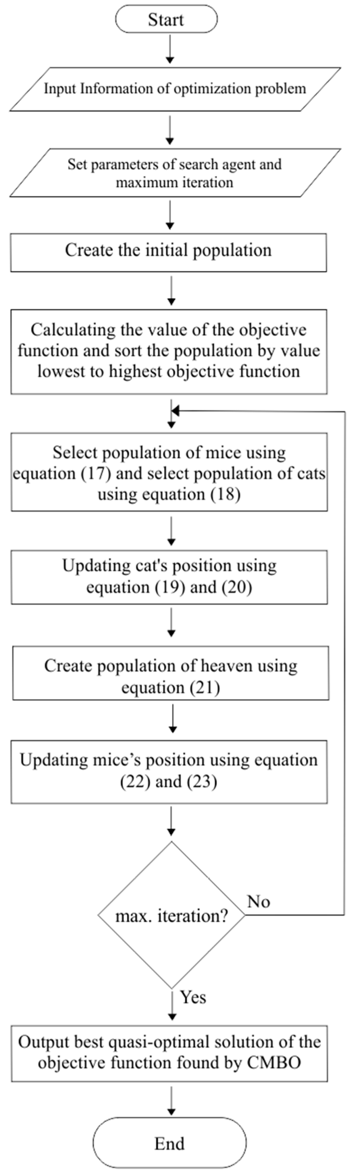
The last stage involves the repetition of the second stage to the fourth stage until the criteria for stopping the CMBO method is met. Conceptually, the stopping criterion in the CMBO method is the maximum iteration obtained, while the optimal CMBO solution is determined based on the population member with the lowest objective value. The CMBO flowchart can be seen in Figure 1.

2.6. Prediction Evaluation

Prediction evaluation was employed to determine the quality of the model developed. In this present study, the evaluation methods utilized include root mean square error (RMSE) and mean absolute percentage error (MAPE). The RMSE was used to evaluate the prediction model by squaring the difference between the actual data and the previous prediction results, divided by the amount of data. The prediction result is considered more accurate when the RMSE value is close to zero [26]:

$$RMSE=\sqrt{\frac{1}{n}{\displaystyle \sum }_{i=1}^n{\left(Y\left(t\right)-\widehat{Y}\left(t\right)\right)}^2}$$

(24)

where $Y\left(t\right)$ is the actual value of the data at time $t$-th, $\widehat{Y}\left(t\right)$ represents the predicted value at time -$t$, and $n$ denotes the data number.

MAPE is a prediction model evaluation method that presents the prediction model error accuracy value in the form of a percentage [6]:

$$MAPE=\frac{1}{n}{\displaystyle \sum }_{t=1}^n\left|\frac{Y\left(t\right)-\widehat{Y}\left(t\right)}{Y\left(t\right)}\right|\times 100\%$$

(25)

where $n$ is the number of data, $Y\left(t\right)$ is the actual data at time t-th, and $\widehat{Y}\left(t\right)$ represents the predicted value at time $t$-th.

Table 1. MAPE Criteria.

MAPE	Prediction Criteria
$<10\%$	Very Accurate
$10\%-20\%$	Accurate
$20\%-50\%$	Reasonable
$>50\%$	Not accurate

shows the standard value prediction criteria for MAPE [27].

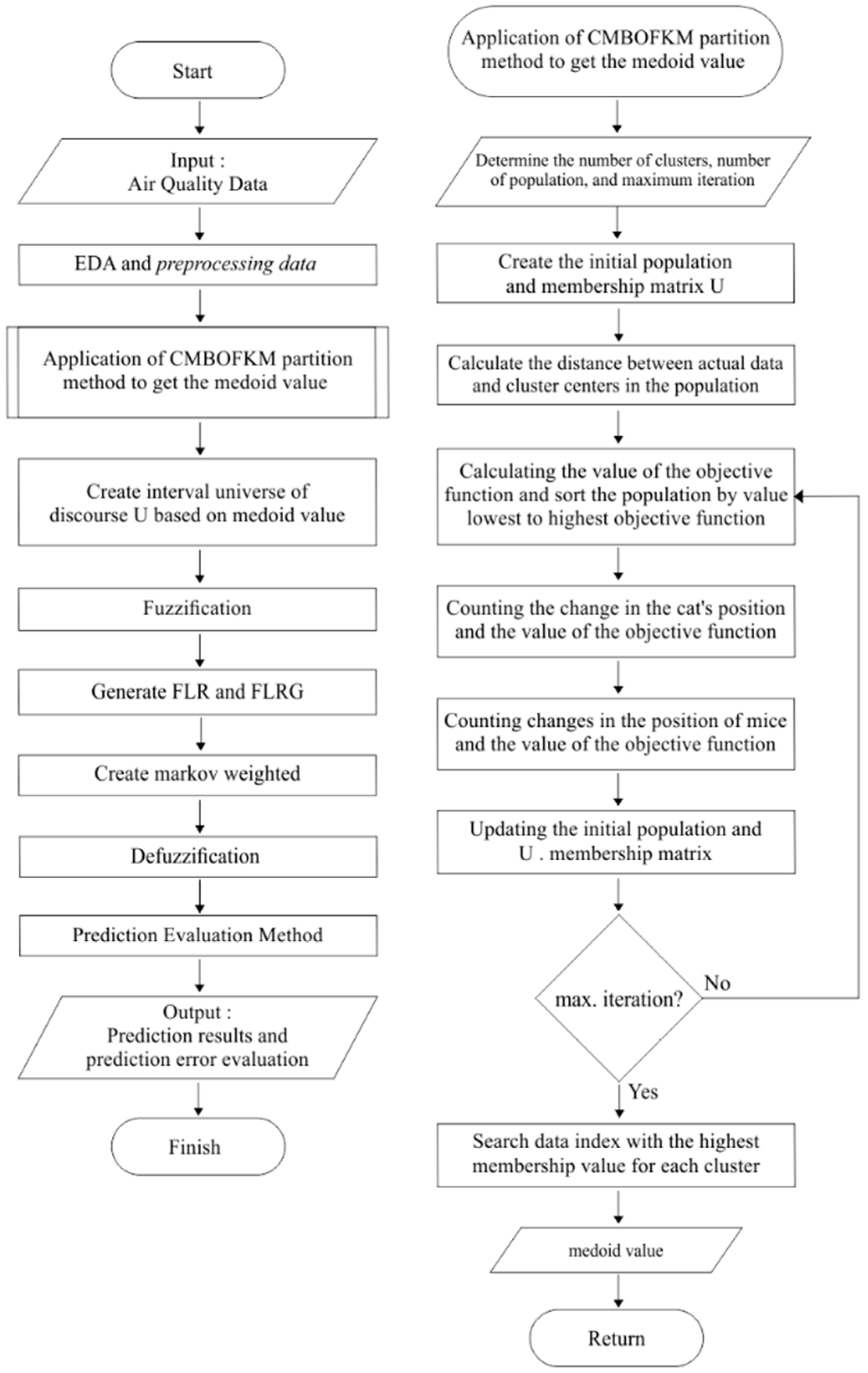
2.7. Flowchart MWFTS-CMBOFKM

The flowchart of the Markov Wighted Fuzzy Time Series model hybridized with CMBOFKM can be seen in Figure 2. First, we enter air quality data and then check the attribute data through EDA and data pre-processing. Data that has gone through EDA and data preprocessing will enter the MWFTS-CMBOFKM model process. In the MWFTS-CMBOFKM Model Algorithm it is divided into 2 important processes, the first is to find the medoid value of the data through the CMBOFKM method, then process the medoid value into U-speech universe intervals to form FLR and FLRG to obtain the predicted value and the results of the prediction model accuracy.

3. Results and Discussion

This study employed the air quality datasets in Klang, Malaysia recorded from 1 January 2020 to 1 May 2022, and the data platform accessed on 9 November 2021 was sourced from the Air Quality Historical Data Platform website on the https://aqicn.org/data-platform/register/. The first dataset used is shown in

Table 2. Air Quality Dataset Klang Malaysia.

Date	AQI
1 January 2020	64
2 January 2020 3 January 2020	64 64
…	…
29 April 2022	47
30 April 2022	50
1 May 2022	50

.

AQI is used to assess air pollution in Malaysia, which was regarded as a simple measure of air quality status. The total number of datasets considered was 852.

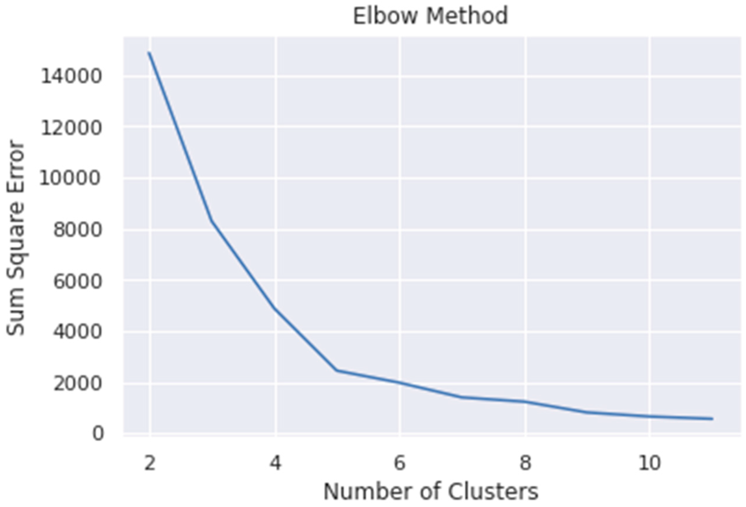
The first step was applying the FKM method with CMBO in order to obtain the medoid value used to form the universe of discourse interval $U$. The selection of parameter values used in this research method has previously been simulated by determining the number of clusters using the elbow method, the number of agents is evaluated based on the lowest MAPE percentage value. The simulation results of the number of clusters used can be seen in Figure 3 while the results of the evaluation of the number of agents based on 100 iterations can be seen in

Table 3. Number of search agents based on MAPE percentage with 100 iteration.

Method	Number of Search Agent
	10	20	30	40
MWFTS-CMBOFKM	7.45%	6.85%	7.68%	9.45%

.

Figure 3 shows that the angled curve is formed when the number of clusters is at five, while Table 3 shows that the smallest MAPE percentage is at 20 search agents, so that the number of clusters used in this study is five, and the number of search agents is 20.

The obtained number of clusters = 5, the initial search agents = 20, and the maximum iteration = 100. The CMBOFKM partition process first generates the membership matrix $U$, while the initial population represents the cluster center.

The membership matrix $U$ was generated based on Equation (8) with a size of $n\times c$ population. This means that each member of the population has their own membership value denoted as $U$. The objective function is also calculated using Equation (7) regarding the populations and the membership matrix $U$. Furthermore, the objective function $\left(P_t\right)$ was sorted from the smallest to the largest values as well as the initial population members and the $U$ membership matrix as shown in

Table 4. The initial population is ordered by the value of the objective function.

Search Agent	${\mathit{V}}_1$	${\mathit{V}}_2$	${\mathit{V}}_3$	${\mathit{V}}_4$	${\mathit{V}}_5$	${\mathit{P}}_1$
Agent 1	$91.14$	$50.44$	$73.20$	$65.28$	$63.89$	$3673.93$
Agent 2	$51.86$	$81.76$	$44.74$	$59.03$	$67.99$	$3843.17$
Agent 3	$66.56$	$52.13$	$109.32$	$58.11$	$75.47$	$4815.71$
$\cdots$	$\cdots$	$\cdots$	$\cdots$	$\cdots$	$\cdots$	$\cdots$
Agent 18	$44.60$	$95.15$	$108.76$	$117.46$	$63.19$	9066.89
Agent 19	$71.13$	$166.84$	$117.33$	$114.16$	$63.88$	9593.49
Agent 20	$117.07$	$94.87$	$110.90$	$86.53$	$86.58$	9796.03

.

The initial population that has been sorted is divided into two equal parts, which include mice and cats populations. Agents 1 to 10 are members of the mouse population, while that of 11 to 20 are the cats. Furthermore, the two populations are updated based on two phases, such as the cat chasing the mouse and the mouse hiding in the nest. The phase of the cat chasing the mouse was determined with Equation (19), while mouse hiding was obtained using Equations (21) and (22). The values of the new objective function in each new population were compared with the old objective function using Equations (20) and (23), and the updated mouse and cat populations are shown in

Table 5. Cat population update results.

Cat Agent	${\mathit{V}}_1$	${\mathit{V}}_2$	${\mathit{V}}_3$	${\mathit{V}}_4$	${\mathit{V}}_5$
Cat 1	$87.90$	$96.21$	$83.00$	$81.04$	$102.95$
Cat 2	$60.00$	$114.97$	$117.51$	$81.42$	$60.05$
Cat 3	$93.83$	$102.05$	$93.33$	$96.91$	$78.44$
$\cdots$	$\cdots$	$\cdots$	$\cdots$	$\cdots$	$\cdots$
Cat 8	$44.60$	$95.15$	$108.76$	$117.46$	$63.19$
Cat 9	$71.13$	$166.84$	$117.33$	$114.16$	$63.88$
Cat 10	$117.07$	$94.87$	$110.90$	$86.53$	$86.58$

and

Table 6. Mice population update results.

Mice Agent	${\mathit{V}}_1$	${\mathit{V}}_2$	${\mathit{V}}_3$	${\mathit{V}}_4$	${\mathit{V}}_5$
Mice 1	$91.14$	$50.44$	$73.20$	$65.28$	$63.89$
Mice 2	$51.86$	$81.76$	$44.74$	$59.03$	$67.99$
Mice 3	$66.56$	$52.13$	$109.32$	$58.11$	$75.47$
$\cdots$	$\cdots$	$\cdots$	$\cdots$	$\cdots$	$\cdots$
Mice 8	$47.49$	$53.10$	$64.42$	$94.67$	$97.96$
Mice 9	$48.97$	$116.85$	$53.78$	$67.80$	$52.58$
Mice 10	$51.24$	$50.48$	$116.29$	$95.43$	$59.39$

.

The updated results of the rat and cat populations are combined into an entirely new population with the newest mouse and cat serving as new members, respectively. Furthermore, the membership matrix $U$ was calculated for each new population member based on Equation (9), and the iteration was performed by sorting the objective values in order to update the membership matrix and a new population regarding the specified maximum iterations.

It is important to note that the maximum iteration in this study was 100, and the membership matrix $U$ was selected based on the search agent with the lowest objective function. Furthermore, the medoid was selected based on the highest membership value in each cluster and was adjusted by sorting the smallest to largest medoid values.

Table 7. Medoid Results of the CMBOFKM partition method.

Cluster	Medoid	Label
Cluster 1	50	Very low
Cluster 2	$64$	Low
Cluster 3	65	Moderate
Cluster 4	$73$	High
Cluster 5	91	Very High

shows the CMBOFKM’s results of the medoid values.

The results of the medoid in

Table 8. The results of the universe of discourse interval $U$ and the middle value.

Interval	Middle Value
$u_1=\left[42,57\right)$	$49.50$
$u_2=\left[57,64.50\right)$	$60.75$
$u_3=\left[64.50,69\right)$	$66.75$
$u_4=\left[69,82\right)$	$75.50$
$u_5=\left[82,119\right)$	$100.50$

are used to form the universe of discourse interval $U$ using Equations (3)–(6) before determining the middle value of each of them. The results of $U$ and middle value are shown in Table 8.

Furthermore, the interval obtained was later entered into the data fuzzification process by changing its value into a fuzzy $A_i$. After fuzzification, the data were in the form of FLR and fuzzy logical relationships group (FLRG) based on Definition 3. The FLRG in the MWFTS method contains the number of transition events from $A_i$ to $A_j \left(i,j=1,2,3,\dots ,c\right)$, while the data fuzzification as well as the formation of FLR and FLRG results are shown in

Table 9. Results of fuzzification of air quality data in Klang, Malaysia.

Date	AQI	Fuzzification	FLR
1 January 2020	$64$	$A_2$	-
2 January 2020	$64$	$A_2$	$A_2\to A_2$
3 January 2020	$64$	$A_2$	$A_2\to A_2$
$\cdots$	$\cdots$	$\cdots$	$\cdots$
29 April 2022	$47$	$A_1$	$A_1\to A_1$
30 April 2022	$50$	$A_1$	$A_1\to A_1$
1 May 2022	$50$	$A_1$	$A_1\to A_1$

and

Table 10. FLRG results.

Group	Fuzzy Logical Group
1	$A_1\to \left(64\right)A_1, \left(55\right)A_2, \left(15\right)A_3,\left(6\right)A_4,\left(1\right)A_5$
2	$A_2\to \left(63\right)A_1,\left(169\right)A_2,\left(55\right)A_3,\left(36\right)A_4,\left(4\right)A_5$
3	$A_3\to \left(7\right)A_1,\left(58\right)A_2,\left(50\right)A_3,\left(38\right)A_4,\left(5\right)A_5$
4	$A_4\to \left(5\right)A_1,\left(40\right)A_2,\left(37\right)A_3,\left(86\right)A_4,\left(18\right)A_5$
5	$A_5\to \left(3\right)A_1,\left(4\right)A_2,\left(1\right)A_3,\left(20\right)A_4,\left(11\right)A_5$

.

Table 10 was used to form a Markov weighted matrix based on Equation (11). The result was expressed as follows:

$$W=\left[\begin{array}{ccccc}0.454& 0.390& 0.106& 0.042& 0.007\\ 0.193& 0.517& 0.168& 0.110& 0.012\\ 0.044& 0.367& 0.316& 0.240& 0.032\\ 0.027& 0.215& 0.199& 0.462& 0.097\\ 0.077& 0.103& 0.026& 0.513& 0.282\end{array}\right]$$

The defuzzification of the predictor value was also calculated based on two stages, namely initial prediction and prediction adjustment. The defuzzification results of the predicted value of MWFTS–CMBOFKM are shown in

Table 11. Defuzzification results of predicted value MWFTS-CMBOFKM.

Date	AQI	Fuzzification	FLR	$\mathit{F}$	$\widehat{\mathit{Y}}$
1 January 2020	$64$	$A_2$	-	-	-
2 January 2020	$64$	$A_2$	$A_2\to A_2$	63.38	63.38
3 January 2020	64	$A_2$	$A_2\to A_2$	63.38	63.38
$\cdots$	$\cdots$	$\cdots$	$\cdots$	$\cdots$	$\cdots$
29 April 2022	$47$	$A_1$	$A_1\to A_1$	$58.33$	$58.33$
30 April 2022	$50$	$A_1$	$A_1\to A_1$	$56.06$	$56.06$
1 May 2022	$50$	$A_1$	$A_1\to A_1$	$57.42$	$57.42$

.

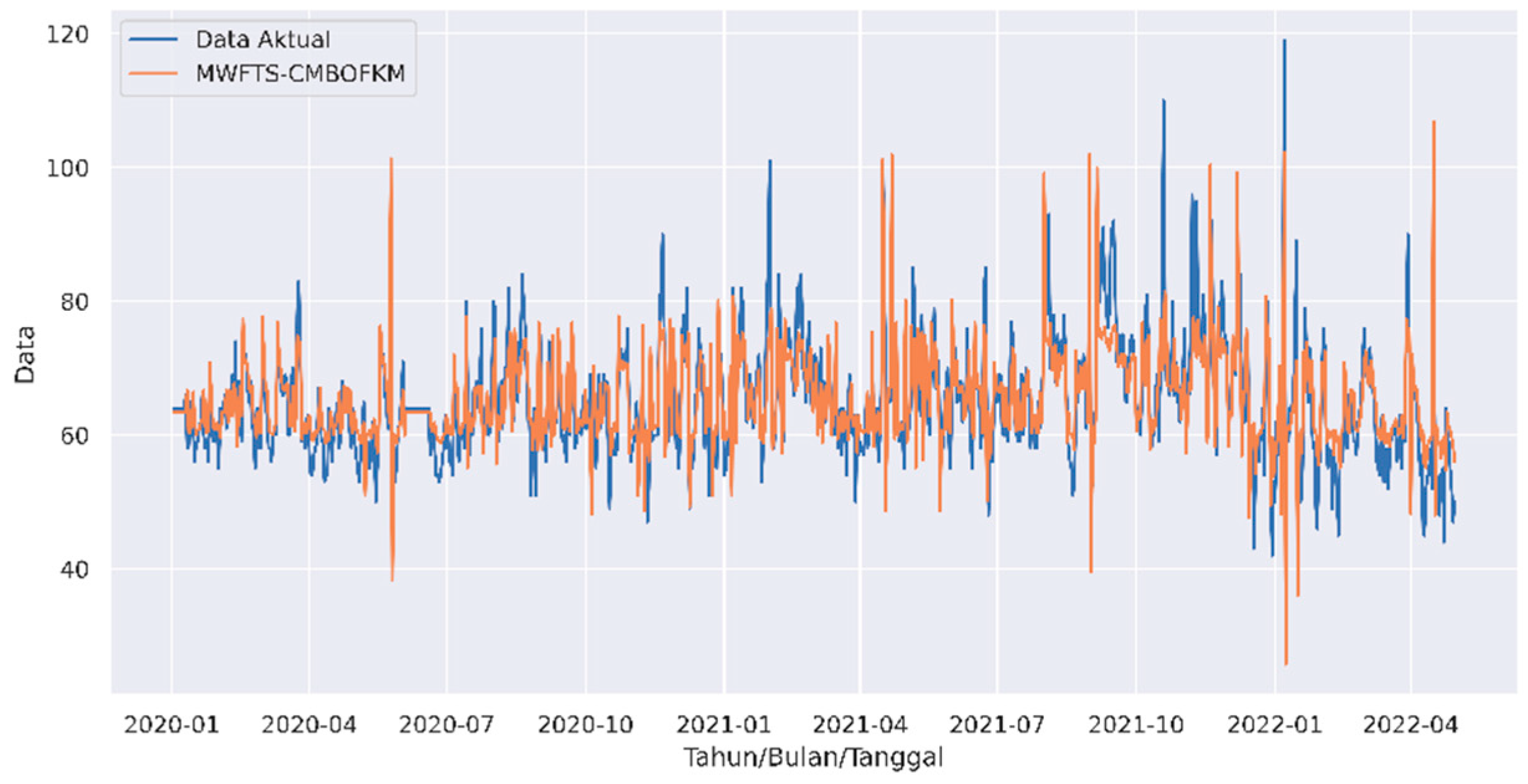
The MWFTS–CMBOFKM prediction results were evaluated based on MAPE and RMSE. It was observed that the method has a MAPE percentage of 6.85% with an RMSE score of 6071. Figure 4 shows the graph comparing the actual data with the predicted results.

According to Figure 4, the MWFTS–CMBOFKM prediction value approaches the actual data value. Meanwhile, the MAPE percentage regarding Table 1 shows that the MWFTS–CMBOFKM prediction model is included in the very accurate prediction criteria.

4. Conclusions

The CMBO method optimizes the FKM cluster center to obtain the best membership matrix $U$ as a producer of the optimal medoid value, which helps to increase the MWFTS predictive accuracy. The implementation of the MWFTS–CMBOFKM method on air quality data in Klang, Malaysia was evaluated using MAPE and RMSE. The results showed that MAPE had a percentage of 6.85%, indicating that the prediction accuracy of MWFTS–CMBOFKM was 93.15% with an RMSE score of 6071. Graphically, it was observed that the predicted value was close to the actual data. Based on Table 1, the MWFTS–CMBOFKM prediction model was very accurate with a MAPE percentage < 10%.

Further studies need to investigate other partitioning methods useful for determining the universe of discourse interval $U$. Furthermore, other population-based optimization methods such as ant colony optimization, bee colony optimization, and the latest population-based optimization methods have to be considered when comparing the resulting level of accuracy.