A Family of 1D Chaotic Maps without Equilibria

Abstract

In this work, a family of piecewise chaotic maps is proposed. This family of maps is parameterized by the nonlinear functions used for each piece of the mapping, which can be either symmetric or non-symmetric. Applying a constraint on the shape of each piece, the generated maps have no equilibria and can showcase chaotic behavior. This family thus belongs to the category of systems with hidden attractors. Numerous examples of chaotic maps are provided, showcasing fractal-like, symmetrical patterns at the interchange between chaotic and non-chaotic behavior. Moreover, the application of the proposed maps to a pseudorandom bit generator is successfully performed.

1. Introduction

Chaos theory is one of the great discoveries of the 20th century. Deterministic chaos as a physical phenomenon is present in many different aspects of nature [1,2]. The field of chaos theory encompasses numerous applications in the natural sciences [3], with contributing research groups from all over the world [4]. One such aspect is chaos-based cryptography. This type of cryptography uses chaotic dynamical systems as a randomness source to perform actions relevant to confusion and diffusion, which are common operations used to encrypt a signal. Due to the determinism of chaos, every action performed on the information signal in order to encrypt it can be reversed at the receiver end to re-obtain the original message.

However, despite the effective use of chaos in encryption, many authors have pointed out some weaknesses in the design of chaotic encryption setups [5,6]. One of the weak points is the chosen chaotic dynamical system, which usually does not have decent properties from the point of view of cryptography. These properties include, among others: a sufficiently large space of possible parameters and initial conditions for which the system is chaotic, appropriate sensitivity to the change of initial conditions and parameters expressed in the form of the Lyapunov exponent, acceptable computational complexity of the algorithm itself, or acceptable complexity of the chaotic dynamical system. Unfortunately, the chaotic systems used in the literature often do not meet all the above-mentioned assumptions.

Currently, chaos-based cryptography is a field of great interest. The interests of researchers include text [7] or image encryption [8], pseudorandom number generators [9,10], methods of generating S-boxes [11], or even asymmetric algorithms [12]. However, chaotic cryptography is not the only application of dynamical systems with chaotic behavior. Other areas where chaotic systems play an important role include secure communications [13], chaotic navigation [14], or optimization [15]. In all these applications, the chaotic systems used should satisfy a certain set of requirements relevant to the application at hand, for example a high key space, uninterrupted chaotic behavior with respect to parameter changes, resistance to parameter estimation attacks, and more.

There are many works on chaotic dynamical systems in the literature. They concern classical systems, such as the logistic map or tent map, and new systems created for the needs of a specific algorithm. However, the newly created systems are often computationally complicated (e.g., they require the use of appropriate numerical methods to generate solutions), or it is difficult to precisely determine for which parameters chaos occurs. Furthermore, in the literature, works on the so-called chaotification can be found, that is, methods of constructing new systems or improving the properties of already existing chaotic systems [16,17,18].

However, many of the new chaotic systems and the chaotification methods do not address the problem of the existence of the fixed points. Fixed points, which are also termed equilibrium points, are problematic because choosing one such point as an initial condition for the system will lead to non-chaotic behavior and thus ruin the design. Moreover, if a fixed point is stable, it will have an attracting region around it, meaning that trajectories starting around a region of the fixed point will also converge to it, again ruining the application performance. Hence, in such situations, the fixed point, along with its basin of attraction, must be excluded from the acceptable set of key values, so as not to ruin the application. A similar situation applies to periodic orbits, which, like fixed points, are not desirable from the point of view of applications. This paper deals with chaotic mappings without fixed points.

Thus, from the point of view of applications, the ideal chaotification method ensures that the system is chaotic, but at the same time, there are no fixed points. The works dealing with this problem concern continuous systems for which the above-mentioned problems occur [19,20,21,22,23,24,25], or for discrete maps, mainly piecewise linear ones [26,27,28,29,30,31,32]. Thus, in work [19], the authors presented a 3D dynamical system, which, apart from the lack of fixed points, is characterized by the coexistence of a limit cycle and torus. In [20], a simple no-equilibrium chaotic system with only one signum function is presented. This system is also characterized by the so-called hidden attractors, which can be distributed in a 1D line, a 2D lattice, or even a 3D grid. In turn, work [21] presents a fractional chaotic system, which is described by equations with few terms and parameters with a minimum of digits. A chaotic fractional dynamical system without fixed points is also shown in [22]. Another chaotic fractional system is also discussed in [23], where apart from the new dynamical system, its synchronization was also presented. In [24], a continuous 3D chaotic dynamical system with no equilibrium and its chaos anti-synchronization was presented. In turn, in [25], the authors present a novel continuous chaotic system without equilibrium. The work shows the dynamics, synchronization, and circuit realization of the proposed system.

Discrete chaotic systems may also not have fixed points. These systems are divided into one-dimensional (1D) systems, usually representing piecewise maps [26,27,28,29] or multidimensional systems [30,31,32]. In [26], a family of 1D piecewise linear maps is proposed, and necessary and sufficient conditions for the absence of equilibria are provided. The mapping region is also tunable by an appropriate parameter choice. In [28], a 1D map from [26] was implemented in an FPGA device. In [29], a new family of 1D maps termed Vertigo was proposed, with a tunable starting period and a period doubling transition to chaos. In [30], two 2D maps with quadratic nonlinearities were proposed, which were not in piecewise form. In [31], a 2D map inspired by the Arnold’s cat map was proposed. In [32], a 2D map was developed combining cosine nonlinearity and a memristor. Finally, work [27] presents a comparative study of recent 1D and 2D maps with and without fixed points. Overall, following the development of continuous time systems, discrete maps without fixed points are receiving more attention in recent years, as more researchers are studying methods of efficiently constructing and studying such systems.

The aim and contribution of this work is the construction of chaotic discrete maps that do not have fixed points. The resulting dynamic systems can be either piecewise linear or nonlinear. The family of maps has three parameters, which are aimed at controlling the shape of each nonlinear piece, so that the map exhibits no fixed points. Three such maps are presented and studied. All maps showcase interesting patterns of transitioning in and out of chaotic behavior, in the space of parameter values. The proposed family of maps has a general form, and thus, numerous maps without equilibria can be generated, meaning that further modifications can be developed in the future. The article also discusses the usefulness of such systems in the area of chaos-based cryptography.

The rest of the work is structured as follows. In Section 2, some fundamental preliminaries are provided regarding discrete maps. Section 3 presents a method for constructing a family of chaotic maps without fixed points. In turn, Section 4 presents examples of maps resulting from the proposed construction along with their analysis. In Section 5, the applications of the obtained chaotic mappings in the context of chaotic cryptography are presented. Section 6 then discusses the conclusions.

2. Preliminaries

In this work, we consider one-dimensional (1D) discrete dynamical systems, described by:

$$x_{k+1}=f\left(x_k\right),$$

(1)

where k denotes the iteration number, $x\left(k\right)$ is the state of the map, and $f(·)$ the mapping function. In this paper, we will consider discrete dynamical systems for which f: $[0,1]\to [0,1]$.

A fixed point, or equilibrium, of a discrete dynamical system Equation (1) is a state value of $x^{*}$ for which the following relation holds

$$f\left(x^{*}\right)=x^{*}.$$

(2)

Graphically, Equation (2) means that the plot of the function $f\left(x\right)$ intersects the bisector line at the point $(x^{*},x^{*})$.

The necessary condition for the occurrence of chaos for mapping Equation (1) is the positive value of the Lyapunov exponent $\lambda$. The value of $\lambda$ for the system Equation (1) is calculated according to the formula

$$\lambda =\underset{n\to \infty }{lim}\frac{1}{n}\sum _{i=0}^{n-1}ln\left|f^{\prime }\left(x_i\right)\right|.$$

(3)

3. The Proposed Family of Maps

Let us consider the following discrete piecewise map

$$x_{k+1}=f\left(x_k\right)=\left\{\begin{array}{cc}(a-1)f_1\left(x_k\right)+1,& 0\le x\le b\\ c{f}_2\left(x_k\right),& b<x\le 1\end{array}\right.,$$

(4)

where $a,b,c\in (0,1)$ are control parameters. Furthermore, $f_1$: $[0,b]\to [0,1]$ and $f_2$: $[b,1]\to [0,1]$ are monotonic continuous functions with boundary values

$$f_1\left(0\right)=1,f_1\left(b\right)=0,$$

(5)

$$f_2\left(b\right)=0,f_2\left(1\right)=1.$$

(6)

The goal is to appropriately select the functions $f_1$, $f_2$ and parameters $a,b$ and c so that Equation (4) has no fixed points.

Examples of functions $f_1$ and $f_2$ and the corresponding dynamical system of the form Equation (4) are shown in Figure 1. Furthermore, this figure clearly shows that each function $f_1$ and $f_2$ has exactly one fixed point (for the function $f_2$, it is the point $x^{*}=1$). In turn, the mapping constructed on their basis does not have such fixed points.

Remark 1.

Map Equation (4) does not have equilibria if none of the functions $f_1\left(x\right)$, $f_2\left(x\right)$ have graphs that intersect with the bisector in the interval $x\in [0,1]$. Equivalently, setting $x_{k+1}=x_k=x^{*}$, the following equations

$$\begin{array}{ccc}\hfill (a-1)f_1\left(x^{*}\right)+1-x^{*}& =& 0,0\le x^{*}\le b\hfill \end{array}$$

(7)

$$\begin{array}{ccc}\hfill \hspace{1em}\hspace{1em}\hspace{1em} c{f}_2\left(x^{*}\right)-x^{*}& =& 0,b<x^{*}\le 1\hfill \end{array}$$

(8)

should not have a solution in the specified intervals.

Remark 2.

Note that the same result can be obtained if the functions $f_1\left(x\right)$ and $f_2\left(x\right)$ are replaced by the functions $g_1\left(x\right)=-f_1\left(x\right)+1$ and $g_2\left(x\right)=-f_2\left(x\right)+1$. Then, the dynamical system takes the form

$$x_{k+1}=g\left(x_k\right)=\left\{\begin{array}{cc}(1-a)g_1\left(x_k\right)+a,& 0\le x\le b\\ -c{g}_2\left(x_k\right)+c,& b<x\le 1\end{array}\right.,$$

(9)

where as before, $a,b,c\in (0,1)$ are control parameters, and $g_1$: $[0,b]\to [0,1],g_2$: $[b,1]\to [0,1]$. Furthermore, $g_1$ and $g_2$ are continuous monotonic functions with boundary values

$$g_1\left(0\right)=0,g_1\left(b\right)=1,$$

(10)

$$g_2\left(b\right)=1,g_2\left(1\right)=0.$$

(11)

Examples of $g_1$ and $g_2$ and the corresponding dynamical system of the form Equation (9) are shown in Figure 2.

Remark 3.

The given construction of mappings without fixed points can be defined in yet another way. Instead of specifying the functions $f_1$ and $f_1$, (or $g_1$ and $g_2$) as shown in the case of mapping Equation (4) (or Equation (9)), it is possible to use the given boundary conditions directly. Then, the construction of mappings will be of the form:

$$x_{k+1}=h\left(x_k\right)=\left\{\begin{array}{cc}{h}_1\left(x_k\right),& 0\le x\le b\\ h_2\left(x_k\right),& b<x\le 1\end{array}\right.,$$

(12)

where $h_1:[0,b]\to [a,1]h_2:[b,1]\to [0,c],a,b,c\in (0,1).$

Furthermore, functions $h_1$ and $h_2$ should satisfy the conditions

$$h_1\left(x\right)>x,\forall x\in [0,b]$$

(13)

$$h_2\left(x\right)<x,\forall x\in [b,1].$$

(14)

The construction of form Equation (12) is more general than the constructions Equation (4) or Equation (9). However, determining functions $h_1$ and $h_2$ may be more difficult in practice. Furthermore, the mappings Equations (4) and (9) can be obtained by using other chaotic systems that are defined in the unit square.

4. Chaotic Map Examples

This section presents three examples illustrating the proposed method for constructing mappings without fixed points. When constructing such maps, the chosen subfunctions of the piecewise mapping can either have symmetry with respect to the family of nonlinear functions they belong, such as polynomial or trigonometric, graphical symmetry with respect to the bisector, or no symmetry at all.

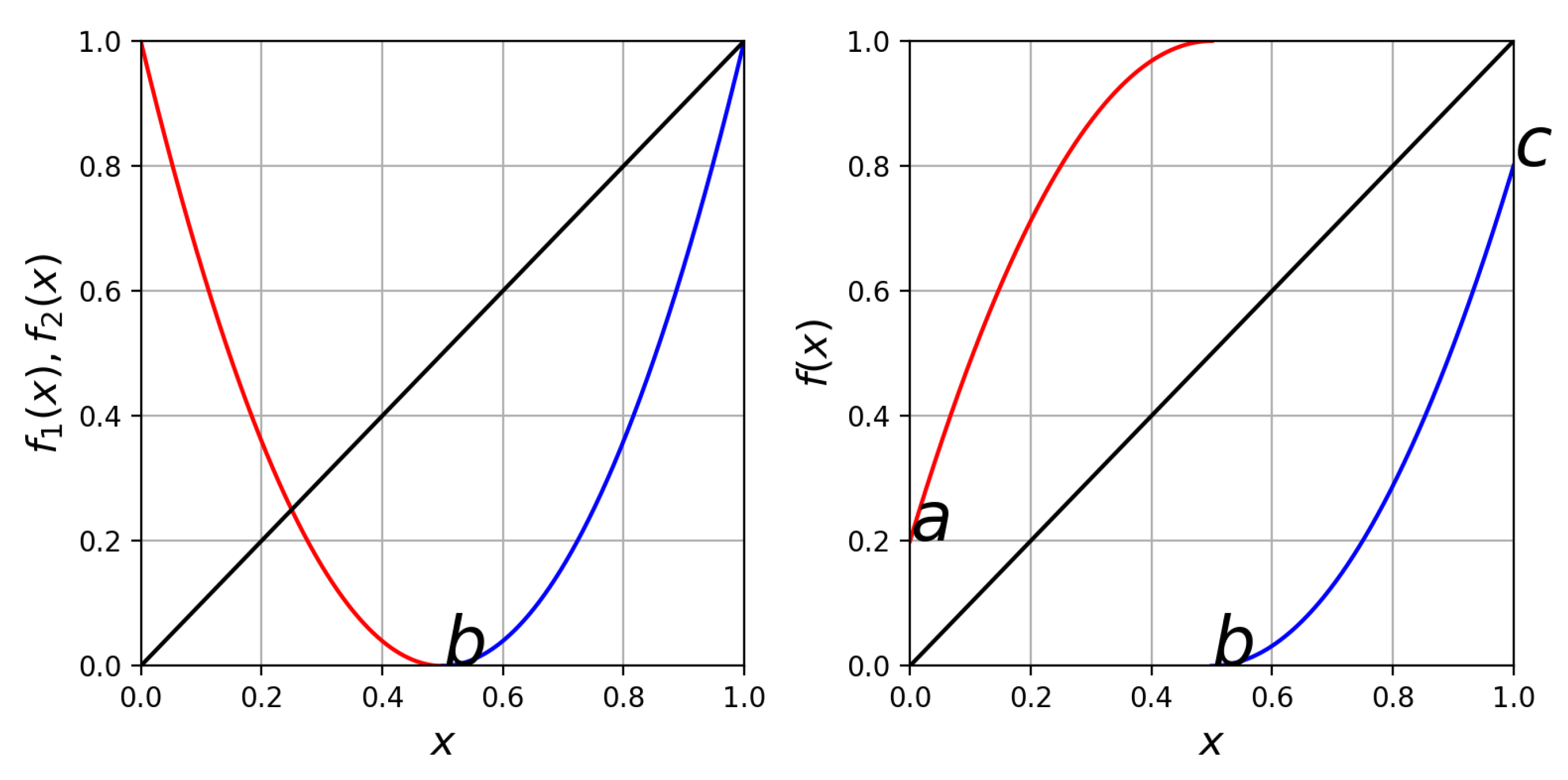
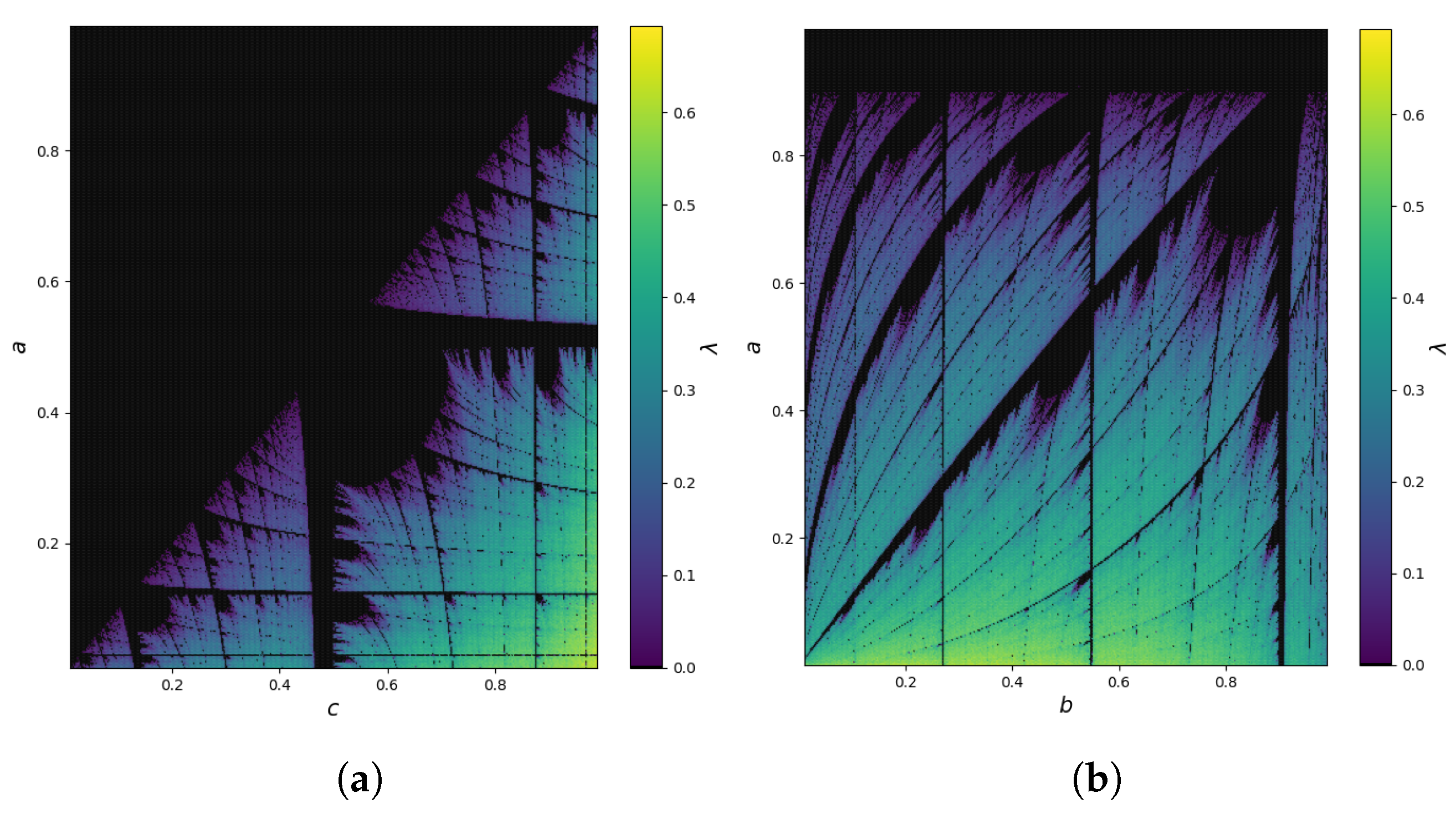
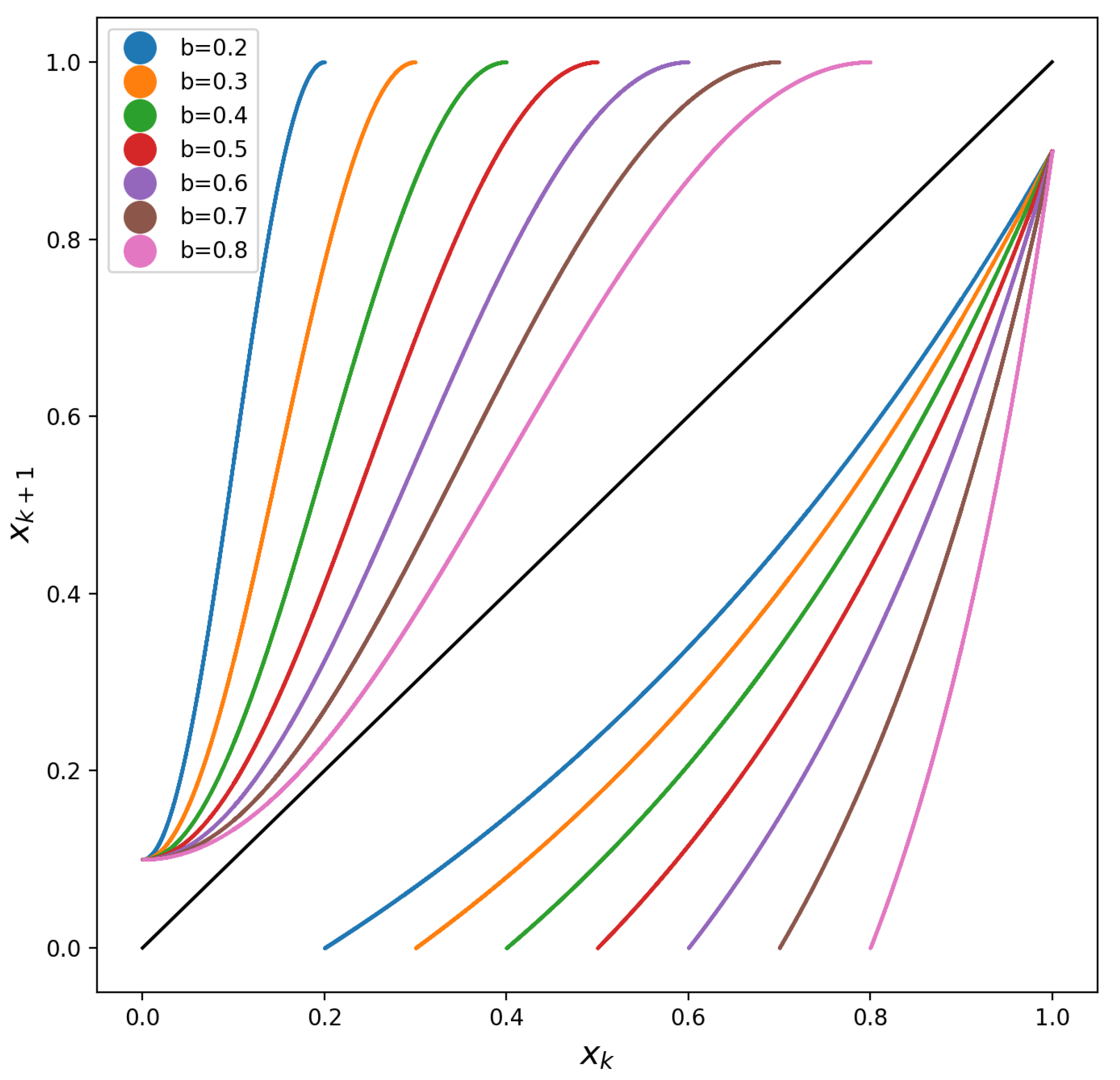
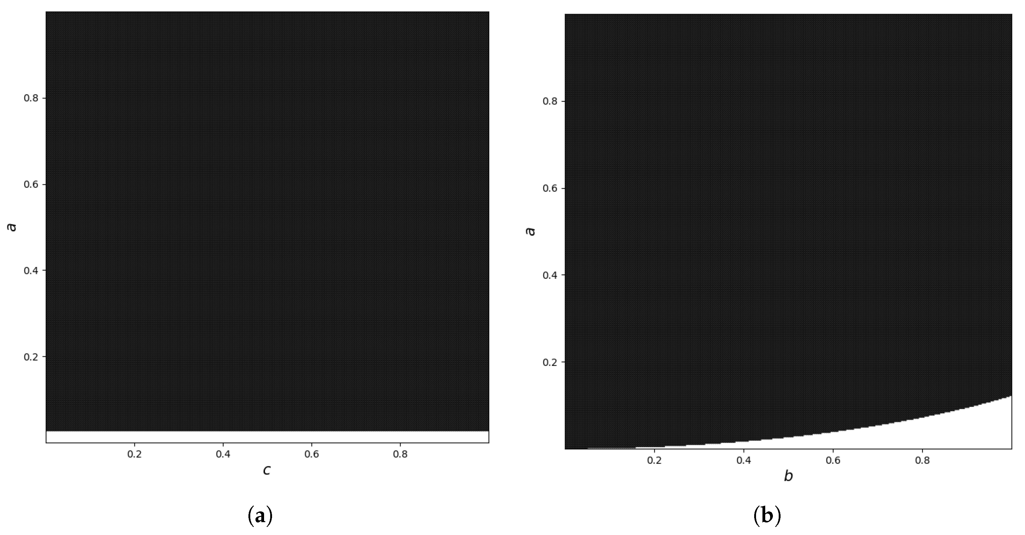
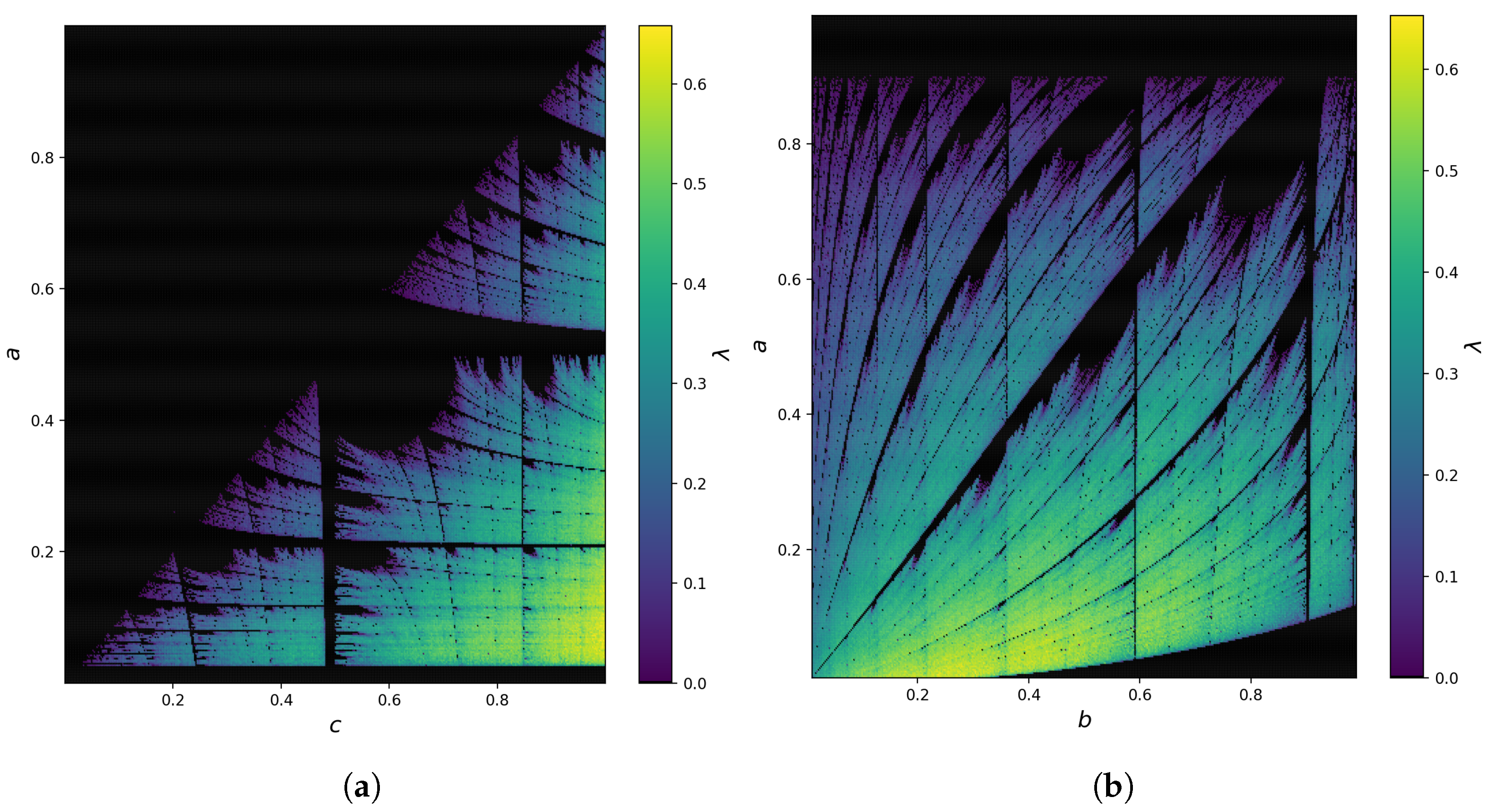
4.1. Example 1—Polynomial Piecewise Map

Let us take the power functions as $f_1$ and $f_2$. Then, the chaotic mapping Equation (4) takes the form:

$$x_{k+1}=\left\{\begin{array}{cc}(a-1){\left(\frac{b-x_k}{b}\right)}^d+1,& 0\le x\le b\\ c{\left(\frac{x_k-b}{1-b}\right)}^d,& b<x\le 1\end{array}\right.,$$

(15)

where $a,b,c\in (0,1),d\in {\mathbb{R}}_{+}.$

Recursion Equation (15) represents a whole family of chaotic maps. Using Remark 2, the asymmetric tent map (then $d=1$ in Equation (15)) or the logistic map (then $d=2$ and $b=0.5$ in Equation (15)—this case is also shown in Figure 2)) can be used as basis functions $g_1$ and $g_2$ to obtain the dynamical system of form Equation (15). Thus, one of the most popular chaotic mappings in the literature can be used to create new dynamical systems.

Lemma 1.

For $d\ge 1$, map Equation (15) has no fixed points.

Proof. 

First, consider the case $d=1$. Then, the recursion functions are linear functions that pass through the points $(0,a)$ and $(b,1)$ for $x\in [0,b]$ and $(b,0)$ and $(1,c)$ for $x\in [b,1]$, respectively. Thus, none of the functions intersect the line $y=x$. This means that for $d=1$, system Equation (15) has no fixed points.

Now consider the case $d>1$. Then, the left function is an increasing continuous concave function that passes through the points $(0,a)$ and $(b,1)$ for $x\in [0,b]$. This conclusion follows directly from the analysis of the properties of the first derivative

$$f^{\prime }\left(x\right)=\frac{-d(a-1)}{b}{\left(\frac{b-x}{b}\right)}^{d-1},$$

(16)

which is positive in the domain, and the second derivative

$$f^{″}\left(x\right)=\frac{d(d-1)(a-1)}{b^2}{\left(\frac{b-x}{b}\right)}^{d-2},$$

(17)

which in this case is negative for $x\in (0,b)$.

In turn, the right function is an increasing continuous convex function that passes through points $(b,0)$ and $(1,c)$ for $x\in (b,1]$. This conclusion also follows directly from the analysis of the properties of the first derivative

$$f^{\prime }\left(x\right)=\frac{dc}{(1-b)}{\left(\frac{x-b}{1-b}\right)}^{d-1},$$

(18)

which is positive in the domain, and the second derivative

$$f^{″}\left(x\right)=\frac{d(d-1)c}{{(1-b)}^2}{\left(\frac{x-b}{1-b}\right)}^{d-2},$$

(19)

which in this case is also positive for $x\in (b,1)$. Thus, none of the functions intersect the line $y=x$. This means that for $d>1$, system Equation (15) has no fixed points. □

Examples of mappings for selected parameter values that meet the assumptions of Lemma 1 are presented, among others, in Figure 3a,b. Figure 3a shows a situation in which different values of parameter b are considered. In turn, Figure 3b shows a situation in which different values of the d parameter were used in Equation (15). Moreover, these mappings are symmetrical.

Remark 4.

For $d<1$, whether map Equation (15) has fixed points or not is determined by the relationships between the parameters $a,b$ and c. This situation is illustrated, among others, in Figure 3b, where for $d=2/3$ or $d=1/3$, the map Equation (15) has no fixed points.

Indicating the relationship when the system has no fixed points analytically can be difficult and, sometimes, even impossible due to the non-linear nature of the mapping. For this purpose, a numerical confirmation of Lemma 1 is shown in Figure 4. The black color shows for which parameter values map Equation (15) has no fixed points. These plots are obtained as follows: the coordinates show whether the functions of map Equation (15) intersect the line $y=x$. If so, such values are marked in white, and if not, in black.

The above remarks refer to the situation in which system Equation (15) has no fixed points. However, this does not mean that its dynamics are chaotic. To check whether map Equation (15) is chaotic, the value of the Lyapunov exponent $\lambda$ should be determined using formula (3). The results obtained are presented in Figure 5. The black color in these plots is the area where the value of the Lyapunov exponent $\lambda$ is not positive. In turn, the other colors show that system Equation (15) is chaotic, and its sensitivity to changes in initial conditions is a fact. In addition, these graphs have a fractal nature, i.e., they are self-similar. This means that it is challenging (if even possible) to give some closed formula to specify when mapping Equation (15) is chaotic and when it is not. Moreover, it can be observed that the graph in Figure 5a is symmetrical.

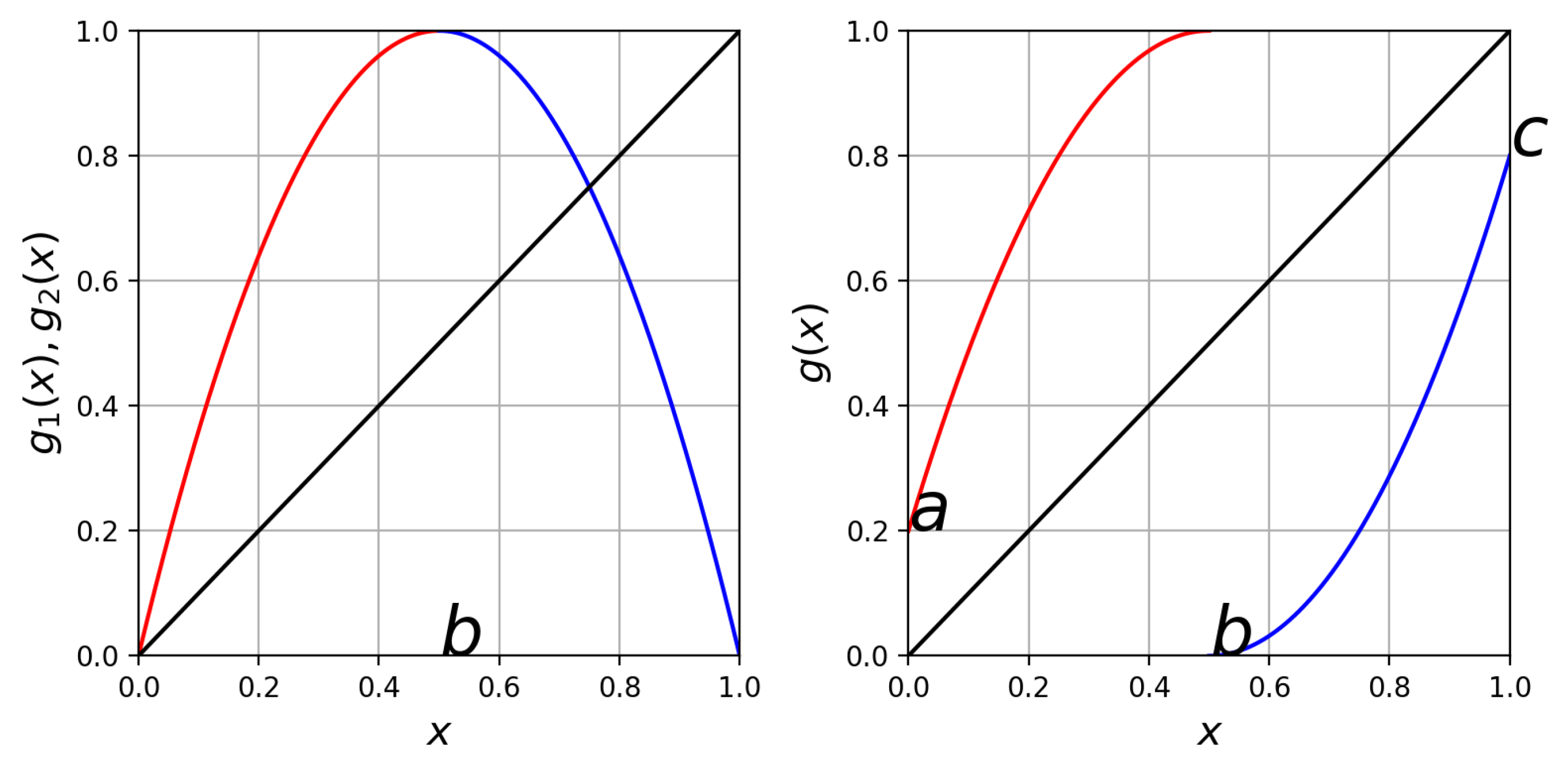
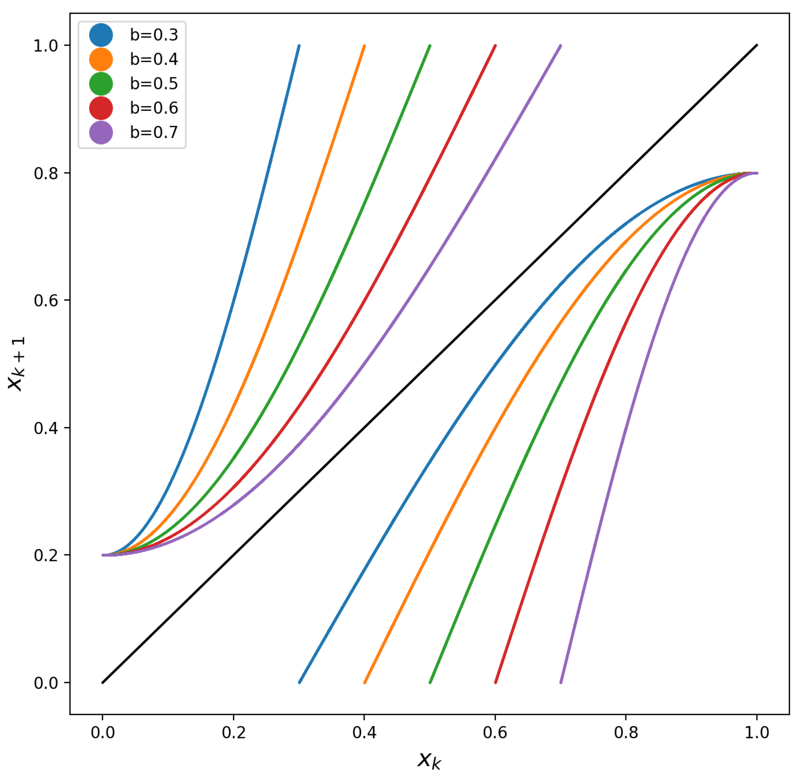
4.2. Example 2—Cosine Piecewise Map

Let us take the $cosine$ functions as $f_1$ and $f_2$. Then, chaotic mapping Equation (4) takes the form:

$$x_{k+1}=\left\{\begin{array}{cc}(a-1)cos\left(\frac{\pi x_k}{2b}\right)+1,& 0\le x\le b\\ ccos\left(\frac{\pi (x_k-1)}{2-2b}\right),& b<x\le 1\end{array}\right.,$$

(20)

where $a,b,c\in (0,1)$.

As in the first example, recursion Equation (20) represents a whole family of chaotic maps. Examples of recursion Equation (20) are shown in Figure 6. The plots of Figure 6 also show that the left and right subfunction of recursion Equation (20) are convex and concave, respectively.

As in the first example, indicating the relationship when the system has no fixed points analytically can be difficult and, sometimes, even impossible due to the non-linear nature of the mapping. Therefore, a numerical analysis of this problem for selected parameter values is shown in Figure 7a,b. The black color shows for which parameter values map Equation (20) has no fixed points. These plots are obtained as in the first example.

By analogy with the first example, the above remarks refer to the situation in which system Equation (20) has no fixed points. However, this does not mean that its dynamics are chaotic. To check whether map Equation (20) is chaotic, the value of the Lyapunov exponent $\lambda$ should be determined using formula (3). The results obtained are presented in Figure 8a,b. The black color in these plots is the area where the value of the Lyapunov exponent $\lambda$ is not positive. In turn, the other colors show that the system Equation (20) is unstable, and its sensitivity to changes in initial conditions is a fact. In addition, these graphs have a fractal nature, i.e., they are self-similar. This means that it is challenging (if even possible) to give some rules when mapping Equation (20) is chaotic and when it is not. Moreover, it can be observed that the graph in Figure 8a is symmetrical.

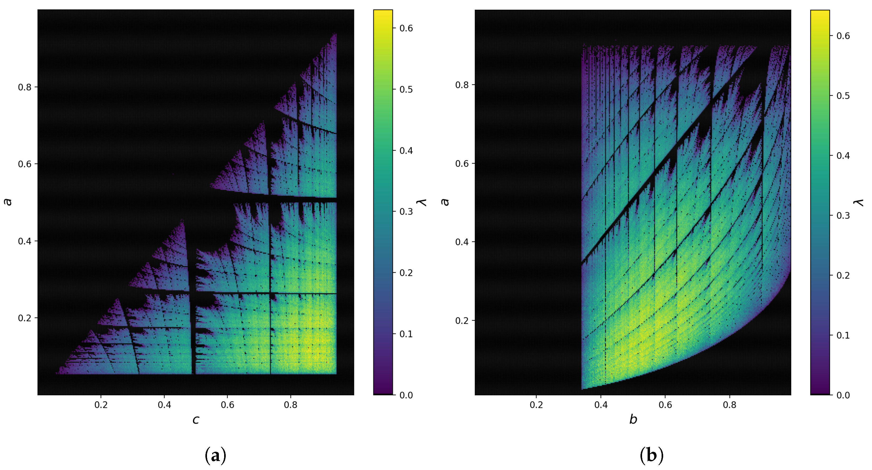
4.3. Example 3—Sine-Exponential Piecewise Map

As a final example, let us take two different functions $f_1$ and $f_2$. Let $f_1$ be the square of the sine function, and let $f_2$ be the exponential function. Then, chaotic mapping Equation (4) takes the form:

$$x_{k+1}=\left\{\begin{array}{cc}(a-1){sin}^2\left(\frac{\pi x_k-\pi b}{2b}\right)+1,& 0\le x\le b\\ \frac{c}{exp\left(1\right)-1}\left(exp\left(\frac{x_k-b}{1-b}\right)-1\right),& b<x\le 1\end{array}\right.,$$

(21)

where $a,b,c\in (0,1)$.

As in the previous examples, recursions Equation (21) represent a whole family of chaotic maps. Examples of recursions Equation (21) are shown in Figure 9. Figure 9 also shows, unlike in the previous examples, that the left subfunction is neither convex nor concave over its entire domain. However, the left subfunction changes its behavior from convex to concave (there is an inflection point). In turn, the right subfunction is convex over its entire domain.

As in the previous examples, indicating the relationship when the system has no fixed points analytically can be difficult and, sometimes, even impossible due to the non-linear nature of the mapping. Therefore, a numerical analysis of this problem for selected parameter values is shown in Figure 10a,b. The black color shows for which parameter values map Equation (21) has no fixed points. These plots are obtained as in the first example.

By analogy with the previous examples, the above remarks refer to the situation in which system Equation (21) has no fixed points. However, this does not mean that its dynamics are chaotic. To check whether map Equation (21) is chaotic, the value of the Lyapunov exponent $\lambda$ should be determined using formula (3). The results obtained are presented in Figure 11a,b. The black color in these plots is the area where the value of the Lyapunov exponent $\lambda$ is not positive. In turn, the other colors show that system Equation (21) is unstable, and its sensitivity to changes in initial conditions is a fact. In addition, these graphs have a fractal nature, i.e., they are self-similar. This means that it is challenging (if even possible) to give some rules when mapping Equation (21) is chaotic and when it is not.

5. Applications of the Proposed Mappings

Chaotic systems find many applications in various engineering areas. One of them is chaotic cryptography. In this area, they can be used as sources in pseudorandom number/bit generators. However, many publications in this area choose continuous multidimensional systems for which chaos occurs with at least three equations describing the system’s dynamics [33,34]. However, such systems in this application area have many disadvantages, for example, the need to use integration methods to obtain solutions, computational complexity, or the difficulty in determining the space of parameter values and initial conditions for which the system behaves chaotically. This makes discrete, one-dimensional systems a better choice in chaotic cryptography. The presented constructions of chaotic mappings Equations (4) and (12) fit perfectly into this application area. The specific presented examples of new mappings do not have the disadvantages mentioned above of multidimensional systems. In turn, their lack of fixed points is undoubtedly a very desirable feature of such dynamical systems. For this reason, the representations of forms Equations (4) and (12) can be used in encryption-related applications.

However, despite the obvious advantages, not all one-dimensional discrete systems are equally good from the point of view of applications. Thus, taking into account the most frequently chosen one-dimensional model in scientific publications, the logistic map, it has many disadvantages from the point of view of applications. One of them is the very limited range of parameter values for which chaos occurs. This disadvantage also applies to many other discrete systems. However, the proposed maps, as can be seen from the Lyapunov exponent graphs, have a fairly large area where the Lyapunov exponent takes a positive value. Furthermore, the proposed construction of mappings, as well as the presented map examples, use at least three parameters (a, b, and c), for which the possibility of chaos occurring is much greater than for mappings with only one parameter.

A Proposed PseudoRandom Bit Generator

As an illustrative example, a pseudorandom bit generator (PRBG) will be designed and tested on all of the considered maps. The PRBG generates 16 bits in each iteration, by hashing the value of the chaotic map through a multiplication and a modulo function. The bit generation in each iteration is given as

$${\mathfrak{B}}_k=\mathrm{de}2\mathrm{bi}(\lfloor (\mathrm{rem}({10}^{12}{x}_k,2^{16})\rfloor ,16),$$

(22)

where de2bi denotes the binary representation of the obtained decimal number, rem is the remainder operator, and $\mathcal{B}=\{{\mathfrak{B}}_1,{\mathfrak{B}}_2,\cdots \}$ is the resulting bitstream. The PRBG generates 16 bits per iteration; thus, in order to generate N bits, the chaotic map must be iterated $\lceil \frac{N}{16}\rceil$ times.

To test the PRBG, the proposed polynomial piecewise map Equation (15), the cosine piecewise map Equation (20), and the sine-exponential piecewise map Equation (21) are considered, with parameters $d=2$, $a=0.1$, $b=0.5$, $c=0.8$ for the first two maps and $a=0.1$, $b=0.5$, $c=0.9$ for the third. For each map, a set of $1000\times {10}^6$ bits are generated, for random initial conditions. Thus, the seed map is initiated for a random $x_0\in (0,1)$, and ${10}^6$ bits are generated using PRBG Equation (22). This process is repeated 1000 times, and the resulting bits are all appended into a single file of $1000\times {10}^6$ digits.

The resulting bitstream is tested through the NIST standard test suite, which consists of 15 statistical tests [35]. The results are shown in

Table 1. NIST test results for PRBG Equation (22) using different maps.

		Map Equation (15)		Map Equation (20)		Map Equation (21)
No.	Test	Ratio	Result	Ratio	Result	Ratio	Result
1	Frequency	990/1000	Pass	990/1000	Pass	987/1000	Pass
2	BlockFrequency	988/1000	Pass	993/1000	Pass	992/1000	Pass
3	CumulativeSums	990/1000	Pass	991/1000	Pass	984/1000	Pass
4	Runs	989/1000	Pass	992/1000	Pass	989/1000	Pass
5	LongestRun	991/1000	Pass	989/1000	Pass	993/1000	Pass
6	Rank	992/1000	Pass	991/1000	Pass	992/1000	Pass
7	FFT	995/1000	Pass	990/1000	Pass	986/1000	Pass
8	NonOverlappingTemplate	990/1000	Pass	988/1000	Pass	990/1000	Pass
9	OverlappingTemplate	990/1000	Pass	994/1000	Pass	990/1000	Pass
10	Universal	987/1000	Pass	986/1000	Pass	987/1000	Pass
11	ApproximateEntropy	985/1000	Pass	983/1000	Pass	995/1000	Pass
12	RandomExcursions	628/634	Pass	626/636	Pass	616/623	Pass
13	RandomExcursionsVariant	626/634	Pass	632/636	Pass	615/623	Pass
14	Serial	987/1000	Pass	988/1000	Pass	989/1000	Pass
15	LinearComplexity	993/1000	Pass	987/1000	Pass	987/1000	Pass

and are successful, meaning that the PRBG Equation (22) with Equation (15), Equation (20) or Equation (21) as a source of randomness can generate sequences that can be considered statistically random. For tests with multiple runs, the last result value is printed.

Note that since the proposed PRBGs used chaotic maps as a source of randomness, the bitstreams will remain aperiodic. Of course, as with all chaotic systems, and digital systems for that matter, the aperiodicity is only limited by the floating point accuracy, which can guarantee sufficiently long aperiodic behavior for the applications in mind. If longer aperiodicity is required, however, the proposed PRBGs can easily be improved by considering available techniques such as parameter perturbation. This technique involves slightly perturbing the map’s parameter after a number of iterations, which can diminish any chance of falling into periodic behavior. Since the maps showcase parameter windows of uninterrupted chaotic behavior, such a technique is applicable.

6. Conclusions

This work considered the construction of piecewise maps without any fixed points. In the numerical examples, polynomial, trigonometrical, and exponential terms were considered, all yielding maps without fixed points, that showcased wide ranges of chaotic behavior and interesting fractal-like patterns in the space of parameters that differentiate between chaotic and nonchaotic behavior.

A major advantage for the proposed family of maps is that it is highly receptive to modifications. The candidate functions $f_1\left(x\right)$, $f_2\left(x\right)$ that can be considered in Equation (4) that satisfy the conditions in Remark 1 are numerous; thus, in addition to the maps already proposed in the Examples section, a plethora of new maps can be constructed. These can be explored in future studies. Moreover, by using the approach proposed in, e.g., Ref. [36], it will be possible to construct new successive chaotic maps without fixed points. In addition, piecewise maps with more than two subfunctions can be constructed, for example by considering techniques similar to the ones developed in [29], in an effort to create robust chaotic maps without fixed points, and with absence of N-periodic behavior.

The methodology proposed in this work can be generalized to a wider family of multidimensional maps. The design constraint for the absence of fixed points is the same and has to be satisfied by each individual state of the map. This is currently under development.

References

1. Strogatz, S.H. Nonlinear Dynamics and Chaos: With Applications to Physics, Biology, Chemistry, and Engineering; CRC Press: Boca Raton, FL, USA, 2018. [Google Scholar]
2. Oestreicher, C. A history of chaos theory. Dialogues Clin. Neurosci. 2007, 9, 279–289. [Google Scholar] [CrossRef] [PubMed]
3. Grassi, G. Chaos in the real world: Recent applications to communications, computing, distributed sensing, robotic motion, bio-impedance modelling and encryption systems. Symmetry 2021, 13, 2151. [Google Scholar] [CrossRef]
4. Akmeşe, Ö.F. Bibliometric Analysis of Publications on Chaos Theory and Applications during 1987–2021. Chaos Theory Appl. 2022, 4, 169–178. [Google Scholar] [CrossRef]
5. Baptista, M.S. Chaos for communication. Nonlinear Dyn. 2021, 105, 1821–1841. [Google Scholar] [CrossRef]
6. Teh, J.S.; Alawida, M.; Sii, Y.C. Implementation and practical problems of chaos-based cryptography revisited. J. Inf. Secur. Appl. 2020, 50, 102421. [Google Scholar] [CrossRef]
7. Lawnik, M.; Moysis, L.; Volos, C. Chaos-Based Cryptography: Text Encryption Using Image Algorithms. Electronics 2022, 11, 3156. [Google Scholar] [CrossRef]
8. Kumar, M.; Saxena, A.; Vuppala, S.S. A survey on chaos based image encryption techniques. In Multimedia Security Using Chaotic Maps: Principles and Methodologies; Springer: Berlin/Heidelberg, Germany, 2020; pp. 1–26. [Google Scholar]
9. Tutueva, A.V.; Nepomuceno, E.G.; Karimov, A.I.; Andreev, V.S.; Butusov, D.N. Adaptive chaotic maps and their application to pseudo-random numbers generation. Chaos Solitons Fractals 2020, 133, 109615. [Google Scholar] [CrossRef]
10. Murillo-Escobar, M.; Cruz-Hernández, C.; Cardoza-Avendaño, L.; Méndez-Ramírez, R. A novel pseudorandom number generator based on pseudorandomly enhanced logistic map. Nonlinear Dyn. 2017, 87, 407–425. [Google Scholar] [CrossRef]
11. Bin Faheem, Z.; Ali, A.; Khan, M.A.; Ul-Haq, M.E.; Ahmad, W. Highly dispersive substitution box (S-box) design using chaos. ETRI J. 2020, 42, 619–632. [Google Scholar] [CrossRef] [Green Version]
12. Shakiba, A. A randomized CPA-secure asymmetric-key chaotic color image encryption scheme based on the Chebyshev mappings and one-time pad. J. King Saud Univ. Comput. Inf. Sci. 2021, 33, 562–571. [Google Scholar] [CrossRef]
13. Rybin, V.; Karimov, T.; Bayazitov, O.; Kvitko, D.; Babkin, I.; Shirnin, K.; Kolev, G.; Butusov, D. Prototyping the Symmetry-Based Chaotic Communication System Using Microcontroller Unit. Appl. Sci. 2023, 13, 936. [Google Scholar] [CrossRef]
14. Artemiou, P.; Moysis, L.; Kafetzis, I.; Bardis, N.G.; Lawnik, M.; Volos, C. Chaotic Agent Navigation: Achieving Uniform Exploration Through Area Segmentation. In Proceedings of the 2022 12th International Conference on Dependable Systems, Services and Technologies (DESSERT), Athens, Greece, 9–11 December 2022; pp. 1–7. [Google Scholar] [CrossRef]
15. Saremi, S.; Mirjalili, S.; Lewis, A. Biogeography-based optimisation with chaos. Neural Comput. Appl. 2014, 25, 1077–1097. [Google Scholar] [CrossRef] [Green Version]
16. Moysis, L.; Lawnik, M.; Antoniades, I.P.; Kafetzis, I.; Baptista, M.S.; Volos, C. Chaotification of 1D Maps by Multiple Remainder Operator Additions—Application to B-Spline Curve Encryption. Symmetry 2023, 15, 726. [Google Scholar] [CrossRef]
17. Natiq, H.; Banerjee, S.; Said, M. Cosine chaotification technique to enhance chaos and complexity of discrete systems. Eur. Phys. J. Spec. Top. 2019, 228, 185–194. [Google Scholar] [CrossRef]
18. Ablay, G. Lyapunov exponent enhancement in chaotic maps with uniform distribution modulo one transformation. Chaos Theory Appl. 2022, 4, 45–58. [Google Scholar] [CrossRef]
19. Wang, Z.; Akgul, A.; Pham, V.T.; Jafari, S. Chaos-based application of a novel no-equilibrium chaotic system with coexisting attractors. Nonlinear Dyn. 2017, 89, 1877–1887. [Google Scholar] [CrossRef]
20. Zhang, S.; Wang, X.; Zeng, Z. A simple no-equilibrium chaotic system with only one signum function for generating multidirectional variable hidden attractors and its hardware implementation. Chaos Interdiscip. J. Nonlinear Sci. 2020, 30, 053129. [Google Scholar] [CrossRef]
21. Cafagna, D.; Grassi, G. Chaos in a new fractional-order system without equilibrium points. Commun. Nonlinear Sci. Numer. Simul. 2014, 19, 2919–2927. [Google Scholar] [CrossRef]
22. Rahman, Z.A.S.A.; Jasim, B.H.; Al-Yasir, Y.I.A.; Abd-Alhameed, R.A.; Alhasnawi, B.N. A New No Equilibrium Fractional Order Chaotic System, Dynamical Investigation, Synchronization, and Its Digital Implementation. Inventions 2021, 6, 49. [Google Scholar] [CrossRef]
23. Ouannas, A.; Khennaoui, A.A.; Momani, S.; Grassi, G.; Pham, V.T. Chaos and control of a three-dimensional fractional order discrete-time system with no equilibrium and its synchronization. AIP Adv. 2020, 10, 045310. [Google Scholar] [CrossRef]
24. Tamba, V.K.; Pham, V.T.; Hoang, D.V.; Jafari, S.; Alsaadi, F.E.; Alsaadi, F.E. Dynamic system with no equilibrium and its chaos anti-synchronization. Automatika 2018, 59, 35–42. [Google Scholar] [CrossRef]
25. Azar, A.T.; Volos, C.; Gerodimos, N.A.; Tombras, G.S.; Pham, V.T.; Radwan, A.G.; Vaidyanathan, S.; Ouannas, A.; Munoz-Pacheco, J.M. A Novel Chaotic System without Equilibrium: Dynamics, Synchronization, and Circuit Realization. Complexity 2017, 2017, 7871467. [Google Scholar] [CrossRef]
26. García-Grimaldo, C.; Campos, E. Chaotic Features of a Class of Discrete Maps without Fixed Points. Int. J. Bifurc. Chaos 2021, 31, 2150200. [Google Scholar] [CrossRef]
27. García-Grimaldo, C.; Campos-Cantón, E. Comparative Analysis of Chaotic Features of Maps Without Fixed Points. In Complex Systems and Their Applications; Huerta Cuéllar, G., Campos Cantón, E., Tlelo-Cuautle, E., Eds.; Springer: Cham, Switzerland, 2022; pp. 151–176. [Google Scholar]
28. García-Grimaldo, C.; Bermudez-Marquez, C.F.; Tlelo-Cuautle, E.; Campos-Cantón, E. FPGA Implementation of a Chaotic Map with No Fixed Point. Electronics 2023, 12, 444. [Google Scholar] [CrossRef]
29. Jafari, S.; Pham, V.T.; Golpayegani, S.M.R.H.; Moghtadaei, M.; Kingni, S.T. The relationship between chaotic maps and some chaotic systems with hidden attractors. Int. J. Bifurc. Chaos 2016, 26, 1650211. [Google Scholar] [CrossRef]
30. Panahi, S.; Sprott, J.C.; Jafari, S. Two simplest quadratic chaotic maps without equilibrium. Int. J. Bifurc. Chaos 2018, 28, 1850144. [Google Scholar] [CrossRef]
31. Wang, C.; Ding, Q. A New Two-Dimensional Map with Hidden Attractors. Entropy 2018, 20, 322. [Google Scholar] [CrossRef] [Green Version]
32. Almatroud, O.A.; Pham, V.T. Building Fixed Point-Free Maps with Memristor. Mathematics 2023, 11, 1319. [Google Scholar] [CrossRef]
33. Nestor, T.; De Dieu, N.J.; Jacques, K.; Yves, E.J.; Iliyasu, A.M.; Abd El-Latif, A.A. A multidimensional hyperjerk oscillator: Dynamics analysis, analogue and embedded systems implementation, and its application as a cryptosystem. Sensors 2019, 20, 83. [Google Scholar] [CrossRef] [Green Version]
34. Zou, C.; Zhang, Q.; Wei, X.; Liu, C. Image encryption based on improved Lorenz system. IEEE Access 2020, 8, 75728–75740. [Google Scholar] [CrossRef]
35. Bassham, L.E.; Rukhin, A.L.; Soto, J.; Nechvatal, J.R.; Smid, M.E.; Barker, E.B.; Leigh, S.D.; Levenson, M.; Vangel, M.; Banks, D.L.; et al. A Statistical Test Suite for Random and Pseudorandom Number Generators for Cryptographic Applications; Sp 800-22 Rev. 1a; National Institute of Standards & Technology: Gaithersburg, MD, USA, 2010. [Google Scholar]
36. Rand, D.; Ostlund, S.; Sethna, J.; Siggia, E.D. Universal transition from quasiperiodicity to chaos in dissipative systems. Phys. Rev. Lett. 1982, 49, 132. [Google Scholar] [CrossRef]
Figure 1. Left: Example of f 1 (red) and f 2 (blue) functions, where f 1 ( x ) = 4 x 1 2 2 for x 0 , 1 2 and f 2 ( x ) = 4 x 1 2 2 for x 1 2 , 1 . Right: map in form Equation (4) with the example functions f 1 and f 2 .
Symmetry 15 01311 g001
Figure 2. Left: Example of g 1 (red) and g 2 (blue) functions, where g 1 ( x ) = 4 x ( 1 x ) for x 0 , 1 2 and g 2 ( x ) = 4 x ( 1 x ) for x 1 2 , 1 . Right: map in form Equation (9) with the example functions g 1 and g 2 .
Symmetry 15 01311 g002
Figure 3. Phase diagrams of map Equation (15). (a) Phase diagrams of map Equation (15) for different b parameter values ( a = 0.1 , c = 0.9 , d = 2 ) . (b) Phase diagrams of map Equation (15) for different d parameter values ( a = 0.1 , b = 0.5 , c = 0.9 ) .
Symmetry 15 01311 g003
Figure 4. Areas without fixed points of map Equation (15) with different parameter relations. (a) Areas (black) without fixed points of map Equation (15) for different a and c parameter values ( b = 0.5 , d = 2 ) . (b) Areas (black) without fixed points of map Equation (15) for different a and b parameter values ( c = 0.9 , d = 2 ) .
Symmetry 15 01311 g004
Figure 5. Lyapunov exponent of map Equation (15) with different parameter relations (black color denotes nonchaotic region). (a) Lyapunov exponent of map Equation (15) for different a and c parameter values ( b = 0.5 , d = 2 ). (b) Lyapunov exponent of map Equation (15) for different a and b parameter values ( c = 0.9 , d = 2 ) .
Symmetry 15 01311 g005
Figure 6. Phase diagram of map Equation (20).
Symmetry 15 01311 g006
Figure 7. Areas without fixed points of map Equation (20) with different parameter relations. (a) Areas (black) without fixed points of Equation (20) for different a and c parameters ( b = 0.5 ) . (b) Areas (black) without fixed points of Equation (20) for different a and b parameters ( c = 0.9 ) .
Symmetry 15 01311 g007
Figure 8. Lyapunov exponent of map Equation (20) with different parameter relations (black color denotes nonchaotic region). (a) Lyapunov exponent of map Equation (20) for different a and c parameters ( b = 0.5 ) . (b) Lyapunov exponent of map Equation (20) for different a and b parameters ( c = 0.9 ) .
Symmetry 15 01311 g008
Figure 9. Phase diagram of map Equation (21).
Symmetry 15 01311 g009
Figure 10. Areas without fixed points on map Equation (21) with different parameter relations. (a) Areas (black) without fixed points of Equation (21) for different a and c parameters ( b = 0.5 ) . (b) Areas (black) without fixed points of Equation (21) for different a and b parameters ( c = 0.9 ) .
Symmetry 15 01311 g010
Figure 11. Lyapunov exponent of map Equation (21) with different parameter relations (black color denotes nonchaotic region). (a) Lyapunov exponent of map Equation (21) for different a and c parameters ( b = 0.5 ) . (b) Lyapunov exponent of map Equation (21) for different a and b parameters ( c = 0.9 ) .
Symmetry 15 01311 g011