
The Unit Alpha-Power Kum-Modified Size-Biased Lehmann Type II Distribution: Theory, Simulation, and Applications


Abstract
1. Introduction
2. Alpha-Power Kum-Modified Size-Biased Lehmann Type II (AP-Kum-MSBL-II) Distribution
3. Mathematical Properties
3.1. Quantile Function
3.2. rth Moments
3.3. Moment-Generating Function (MGF)
3.4. Mean and Variance
3.5. Stress–Strength Reliability
4. Maximum Likelihood Estimation
5. Bayesian Estimators
5.1. Prior Distribution and Loss Function
5.2. Posterior Analysis
6. Simulation
- Establish the sample size and the beginning parameter values.
- Create an n-sized random sample from the AP-Kum-MSBL-II distribution.
- For MLE, the Newton–Raphson iterative approach is used to solve non-linear equations using the “maxLik” package in the R program. For Bayesian estimation, MCMC is used to solve the complex integration using the “coda” package in the R program.
- Calculate the average estimates, along with their mean squared errors (MSE), relative biases (RB), length of asymptotic confidence intervals (LACI), and coverage probability (CP) with 95%.
- Perform the above two steps 5000 times.
- The provided estimates of , and offer good performance, which is the key general point.
- All estimates perform satisfactorily as n increases.
- Based on the gamma information, the Bayes estimates of , and behaved more predictably than the MLE estimate. Regarding the HPD credible intervals, the same statement might be made.
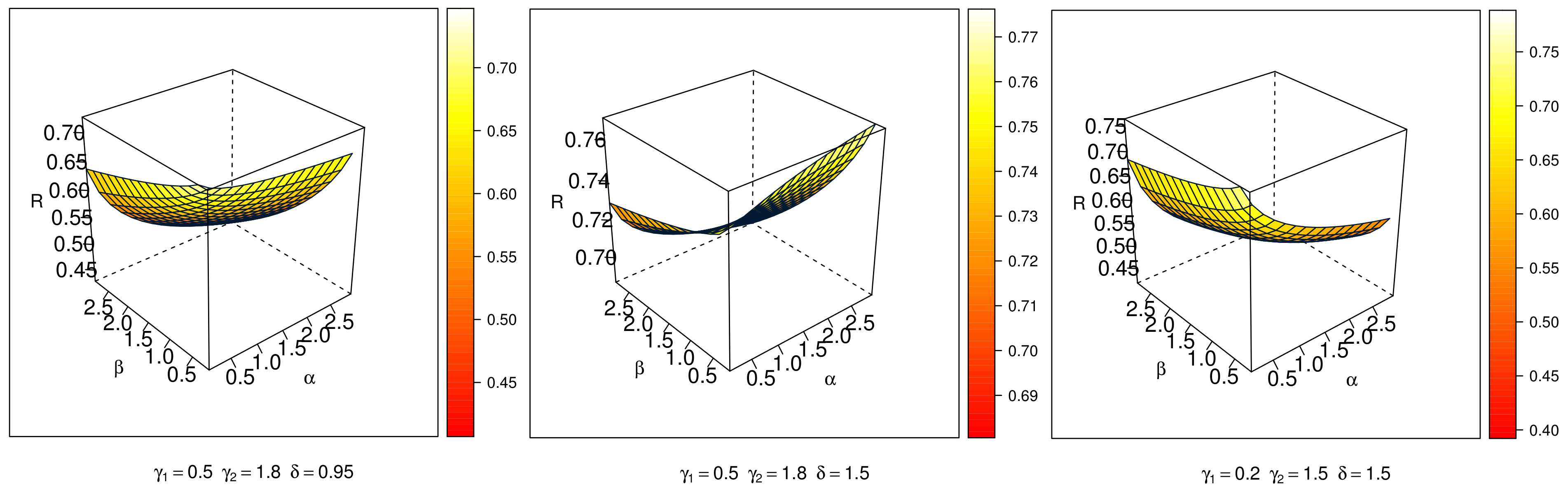
- When increases, the measures of , , and increase, and the measure of decreases.
- In some cases, when increases, the measures of all parameters decrease.
7. Applications
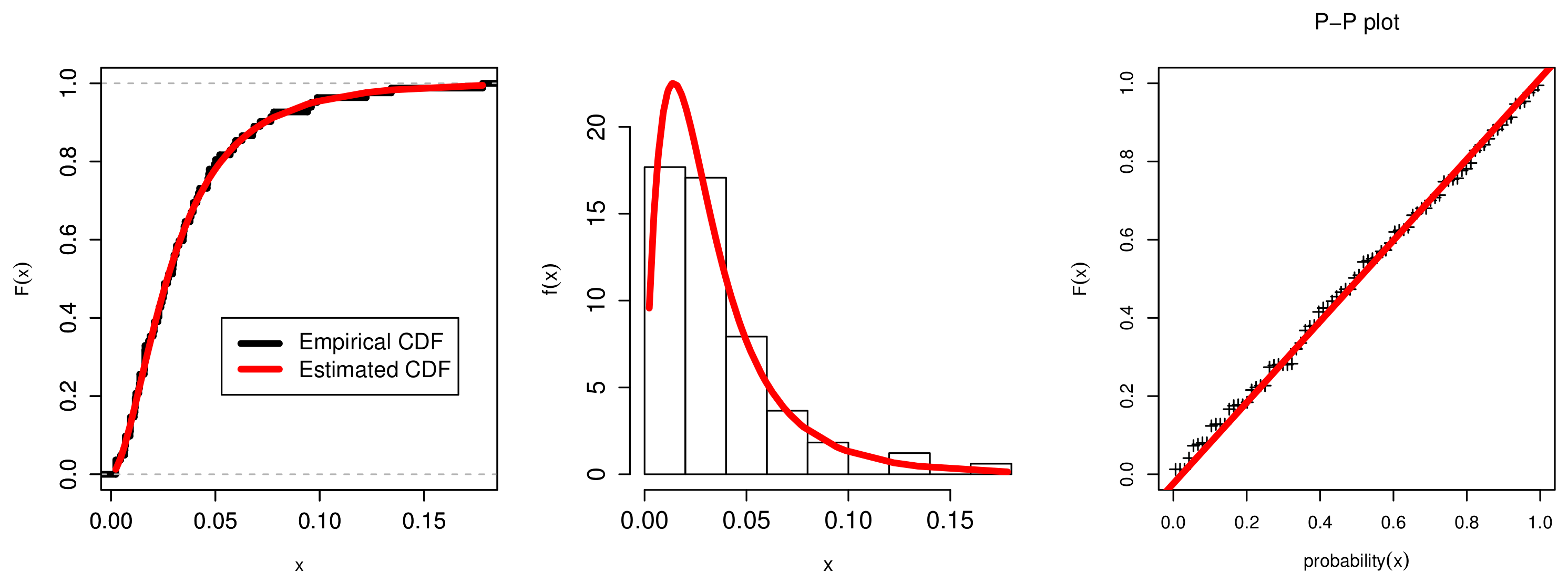
7.1. The COVID-19 Application
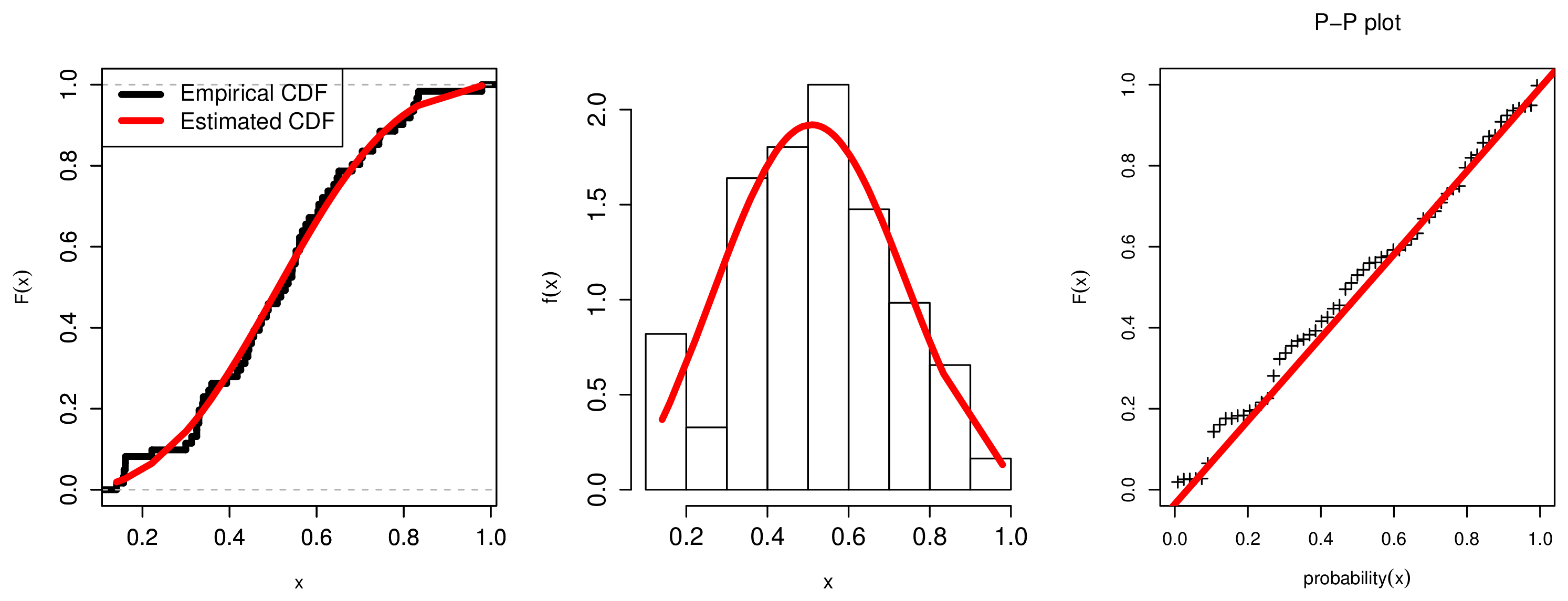
7.2. Determinants of Economic Development Application
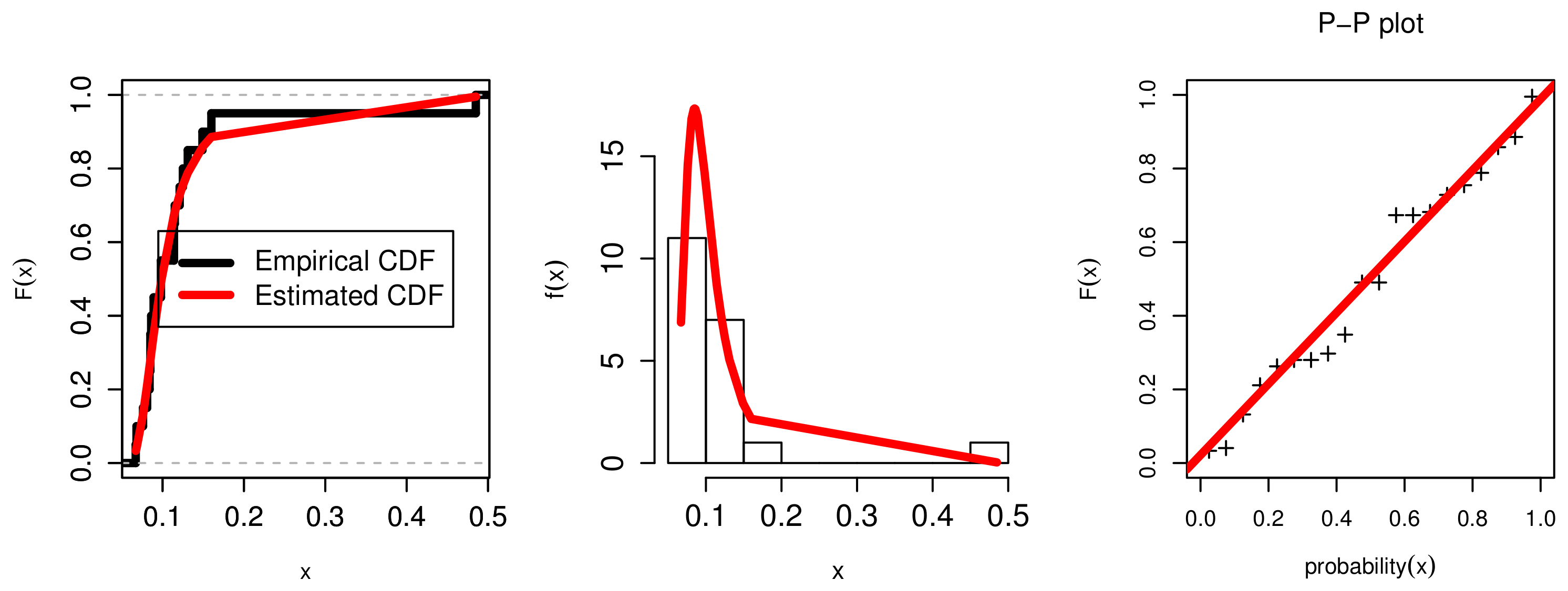
7.3. The Failure Rates Application
8. Conclusions
Author Contributions
Funding
Data Availability Statement
Acknowledgments
Conflicts of Interest
References
- Alsadat, N.; Hassan, A.S.; Elgarhy, M.; Chesneau, C.; Mohamed, R.E. An Efficient Stress–Strength Reliability Estimate of the Unit Gompertz Distribution Using Ranked Set Sampling. Symmetry 2023, 15, 1121. [Google Scholar] [CrossRef]
- Alghamdi, S.M.; Shrahili, M.; Hassan, A.S.; Gemeay, A.M.; Elbatal, I.; Elgarhy, M. Statistical Inference of the Half Logistic Modified Kies Exponential Model with Modeling to Engineering Data. Symmetry 2023, 15, 586. [Google Scholar] [CrossRef]
- Ghaderinezhad, F.; Ley, C.; Loperfido, N. Bayesian inference for skew-symmetric distributions. Symmetry 2020, 12, 491. [Google Scholar] [CrossRef]
- Ramadan Ahmed, T.; Tolba Ahlam, H.; El-Desouky Beih, S.A. Unit half-logistic geometric distribution and its application in insurance. Axioms 2022, 11, 676. [Google Scholar] [CrossRef]
- Dey, S.; Nassar, M.; Kumar, D. Alpha power transformed inverse Lindley distribution: A distribution with an upside-down bathtub-shaped hazard function. J. Comput. Appl. Math. 2019, 348, 130–145. [Google Scholar] [CrossRef]
- Mazucheli, J.; Menezes, A.F.B.; Ghitany, M.E. The unit-Weibull distribution and associated inference. J. Appl. Probab. Stat. 2018, 13, 1–22. [Google Scholar]
- Mazucheli, J.; Menezes, A.F.B.; Fernandes, L.B.; De Oliveira, R.P.; Ghitany, M.E. The unit-Weibull distribution as an alternative to the Kumaraswamy distribution for the modeling of quantiles conditional on covariates. J. Appl. Stat. 2020, 47, 954–974. [Google Scholar] [CrossRef]
- Mazucheli, J.; Menezes, A.F.B.; Chakraborty, S. On the one parameter unit-Lindley distribution and its associated regression model for proportion data. J. Appl. Stat. 2019, 46, 700–714. [Google Scholar] [CrossRef]
- Alzaatreh, A.; Lee, C.; Famoye, F. A new method for generating families of continuous distributions. Metron 2013, 71, 63–79. [Google Scholar] [CrossRef]
- Lee, C.; Famoye, F.; Alzaatreh, A.Y. Methods for generating families of univariate continuous distributions in the recent decades. Wiley Interdiscip. Rev. Comput. Stat. 2013, 5, 219–238. [Google Scholar] [CrossRef]
- Lemonte, A.J.; Cordeiro, G.M.; Ortega, E.M. On the additive Weibull distribution. Commun. Stat. Theory Methods 2014, 43, 2066–2080. [Google Scholar] [CrossRef]
- Sarhan, A.M.; Apaloo, J. Exponentiated modified Weibull extension distribution. Reliab. Eng. Syst. Saf. 2013, 112, 137–144. [Google Scholar] [CrossRef]
- Sarhan, A.M. A two-parameter discrete distribution with a bathtub hazard shape. Commun. Stat. Appl. Methods 2017, 24, 15–27. [Google Scholar] [CrossRef]
- Sarhan, A.M.; Hamilton, D.C.; Smith, B. Parameter estimation for a two-parameter bathtub-shaped lifetime distribution. Appl. Math. Model. 2012, 36, 5380–5392. [Google Scholar] [CrossRef]
- Tolba, A.H. Bayesian and Non-Bayesian Estimation Methods for Simulating the Parameter of the Akshaya Distribution. Comput. J. Math. Stat. Sci. 2022, 1, 13–25. [Google Scholar] [CrossRef]
- Tolba, A.H.; Almetwally, E.M. Bayesian and Non-Bayesian Inference for The Generalized Power Akshaya Distribution with Application in Medical. Comput. J. Math. Stat. Sci. 2023, 2, 31–51. [Google Scholar]
- Sarhan, A.M.; Smith, B.; Hamilton, D.C. Estimation of P (Y < X) for a two-parameter bathtub shaped failure rate distribution. Int. J. Stat. Probab. 2015, 4, 33–45. [Google Scholar]
- Ramadan, D.A.; Magdy, A.W. On the Alpha-Power Inverse Weibull Distribution. Int. J. Comput. Appl. 2018, 181, 6–12. [Google Scholar]
- Mahdavi, A.; Kundu, D. A new method for generating distributions with an application to an exponential distribution. Commun. Stat. Theory Methods 2017, 46, 6543–6557. [Google Scholar] [CrossRef]
- Dey, S.; Alzaatreh, A.; Zhang, C.; Kumar, D. A new extension of generalized exponential distribution with application to Ozone data. Ozone Sci. Eng. 2017, 39, 273–285. [Google Scholar] [CrossRef]
- Mahmood, Z.; Jawa, T.M.; Sayed-Ahmed, N.; Khalil, E.M.; Muse, A.H.; Tolba, A.H. An extended cosine generalized family of distributions for reliability modeling: Characteristics and applications with simulation study. Math. Probl. Eng. 2022, 2022, 3634698. [Google Scholar] [CrossRef]
- Muse, A.H.; Tolba, A.H.; Fayad, E.; Abu Ali, O.A.; Nagy, M.; Yusuf, M. Modelling the COVID-19 mortality rate with a new versatile modification of the log-logistic distribution. Comput. Intell. Neurosci. 2021, 2021, 8640794. [Google Scholar] [CrossRef] [PubMed]
- Al-Babtain, A.A.; Elbatal, I.; Chesneau, C.; Jamal, F. The transmuted Muth generated class of distributions with applications. Symmetry 2020, 12, 1677. [Google Scholar] [CrossRef]
- Jodra, P.; Gomez, H.W.; Jimenez-Gamero, M.D.; Alba-Fernandez, M.V. The power Muth distribution. Math. Model. Anal. 2017, 22, 186–201. [Google Scholar] [CrossRef]
- Alanzi, A.R.A.; Rafique, M.Q.; Tahir, M.H.; Jamal, F.; Hussain, M.A.; Sami, W. A novel Muth generalized family of distributions: Properties and applications to quality control. AIMS Math. 2023, 8, 6559–6580. [Google Scholar] [CrossRef]
- Irshad, M.R.; Maya, R.; Krishna, A. Exponentiated power Muth distribution and associated inference. J. Indian Soc. Probab. Stat. 2021, 22, 265–302. [Google Scholar] [CrossRef]
- Chesneau, C.; Agiwal, V. Statistical theory and practice of the inverse power Muth distribution. J. Comput. Math. Data Sci. 2021, 1, 100004. [Google Scholar] [CrossRef]
- Almarashi, A.M.; Jamal, F.; Chesneau, C.; Elgarhy, M. A new truncated muth generated family of distributions with applications. Complexity 2021, 2021, 1211526. [Google Scholar] [CrossRef]
- Jäntschi, L. Detecting extreme values with order statistics in samples from continuous distributions. Mathematics 2020, 8, 216. [Google Scholar] [CrossRef]
- Krishna, A.; Maya, R.; Chesneau, C.; Irshad, M.R. The Unit Teissier Distribution and Its Applications. Math. Comput. Appl. 2022, 27, 12. [Google Scholar] [CrossRef]
- Nassar, M.; Alzaatreh, A.; Mead, M.; Abo-Kasem, O. Alpha power Weibull distribution: Properties and applications. Commun. Stat. Theory Methods 2017, 46, 10236–10252. [Google Scholar] [CrossRef]
- Hassan, A.S.; Mohamed, R.E.; Elgarhy, M.; Fayomi, A. Alpha power transformed extended exponential distribution: Properties and applications. J. Nonlinear Sci. Appl. 2018, 12, 62–67. [Google Scholar] [CrossRef]
- Lehmann, E.L. The Power of Rank Tests. Ann. Math. Stat. 1953, 24, 23–43. [Google Scholar] [CrossRef]
- Balogun, O.S.; Iqbal, M.Z.; Arshad, M.Z.; Afify, A.Z.; Oguntunde, P.E. A new generalization of Lehmann type-II distribution: Theory, simulation, and applications to survival and failure rate data. Sci. Afr. 2021, 12, e00790. [Google Scholar] [CrossRef]
- Zhuang, L.; Xu, A.; Wang, X.-L. A prognostic driven predictive maintenance framework based on Bayesian deep learning. Reliab. Eng. Syst. Saf. 2023, 234, 109181. [Google Scholar] [CrossRef]
- Luo, C.; Shen, L.; Xu, A. Modelling and estimation of system reliability under dynamic operating environments and lifetime ordering constraints. Reliab. Eng. Syst. Saf. 2022, 218, 108136. [Google Scholar] [CrossRef]
- Xu, A.; Zhou, S.; Tang, Y. A unified model for system reliability evaluation under dynamic operating conditions. IEEE Trans. Reliab. 2019, 70, 65–72. [Google Scholar] [CrossRef]
- Bernardo, J.M.; Smith, A.F.M. Bayesian Theory; Wiley: New York, NY, USA, 1994; Volume 49. [Google Scholar]
- Al-Babtain, A.A.; Elbatal, I.; Almetwally, E.M. Bayesian and Non-Bayesian Reliability Estimation of Stress-Strength Model for Power-Modified Lindley Distribution. J. Comput. Intell. Neurosci. 2022, 2022, 1154705. [Google Scholar] [CrossRef]
- Yousef, M.M.; Almetwally, E.M. Bayesian Inference for the Parameters of Exponentiated Chen Distribution Based on Hybrid Censoring. Pak. J. Statist. 2022, 38, 145–164. [Google Scholar]
- Calabria, R.; Pulcini, G.S. An engineering approach to Bayes estimation for the Weibull distribution. Microelectron. Reliab. 1994, 34, 789–802. [Google Scholar] [CrossRef]
- Abu El Azm, W.S.; Almetwally, E.M.; Naji AL-Aziz, S.; El-Bagoury, A.A.A.H.; Alharbi, R.; Abo-Kasem, O.E. A new transmuted generalized Lomax distribution: Properties and applications to COVID-19 data. Comput. Intell. Neurosci. 2021, 2021, 5918511. [Google Scholar] [CrossRef] [PubMed]
- Anderson, D.R.; Burnham, K.P.; White, G.C. Comparison of Akaike information criterion and consistent Akaike information criterion for model selection and statistical inference from capture-recapture studies. J. Appl. Stat. 1998, 25, 263–282. [Google Scholar] [CrossRef]
- Bierens, H.J. Information Criteria and Model Selection; Penn State University: State College, PA, USA, 2004. [Google Scholar]
- Stock, J.H.; Watson, M.W. Introduction to Econometrics; Addison Wesley: Boston, MA, USA, 2003; Volume 104. [Google Scholar]
- Murthy, D.P.; Xie, M.; Jiang, R. Weibull Models; John Wiley & Sons: Hoboken, NJ, USA, 2004. [Google Scholar]


| MLE | SELF | ELF b = 0.5 | ELF b = 1.5 | |||||||||||||
|---|---|---|---|---|---|---|---|---|---|---|---|---|---|---|---|---|
| n | RB | MSE | LACI | CP | RB | MSE | LCCI | RB | MSE | LCCI | RB | MSE | LCCI | |||
| 1 | 0.6 | 30 | 0.7811 | 0.6756 | 2.8365 | 95.60% | 0.2437 | 0.1681 | 1.2929 | 0.1757 | 0.1387 | 1.2184 | 0.0536 | 0.0975 | 1.0990 | |
| 0.2140 | 0.0776 | 0.9696 | 95.30% | 0.1570 | 0.0326 | 0.4828 | 0.1422 | 0.0284 | 0.4680 | 0.1142 | 0.0219 | 0.4271 | ||||
| 0.0056 | 0.1398 | 1.4665 | 96.10% | 0.2367 | 0.1305 | 1.3576 | 0.1734 | 0.1828 | 1.4589 | 0.0657 | 0.1222 | 1.2758 | ||||
| 0.5052 | 0.3079 | 1.8228 | 94.40% | 0.2934 | 0.2047 | 1.4234 | 0.2325 | 0.1668 | 1.3273 | 0.1235 | 0.1129 | 1.1667 | ||||
| 75 | 0.7087 | 0.4559 | 2.2544 | 94.40% | 0.2648 | 0.1086 | 1.0929 | 0.2136 | 0.0908 | 1.0358 | 0.1204 | 0.0654 | 0.9570 | |||
| 0.1123 | 0.0209 | 0.5019 | 95.60% | 0.0679 | 0.0048 | 0.1873 | 0.0642 | 0.0044 | 0.1820 | 0.0570 | 0.0039 | 0.1755 | ||||
| 0.0714 | 1.0473 | 96.50% | 0.0197 | 0.0716 | 1.0481 | 0.0494 | 0.0714 | 0.9367 | 0.0167 | 0.0610 | 0.9168 | |||||
| 0.3854 | 0.1639 | 1.3036 | 95.70% | 0.2468 | 0.1487 | 1.2876 | 0.2005 | 0.1245 | 1.1896 | 0.1173 | 0.0888 | 1.0586 | ||||
| 150 | 0.4254 | 0.1970 | 1.5279 | 94.80% | 0.2593 | 0.0753 | 0.8429 | 0.2263 | 0.0643 | 0.7983 | 0.1641 | 0.0466 | 0.7087 | |||
| 0.0982 | 0.0103 | 0.3247 | 96.00% | 0.0366 | 0.0013 | 0.0875 | 0.0354 | 0.0012 | 0.0873 | 0.0330 | 0.0011 | 0.0869 | ||||
| 0.0371 | 0.7420 | 95.60% | 0.0152 | 0.0351 | 0.6914 | 0.0412 | 0.0698 | 0.6808 | 0.0106 | 0.0305 | 0.6091 | |||||
| 0.3195 | 0.0753 | 0.7697 | 94.50% | 0.2250 | 0.0611 | 0.6110 | 0.1903 | 0.0698 | 0.7059 | 0.1265 | 0.0726 | 0.5947 | ||||
| 2 | 30 | 0.9482 | 1.0988 | 3.6666 | 94.20% | 0.2485 | 0.1859 | 1.4234 | 0.1812 | 0.1528 | 1.3329 | 0.0613 | 0.1070 | 1.1677 | ||
| 0.1647 | 0.0474 | 0.7605 | 95.70% | 0.1284 | 0.0235 | 0.4659 | 0.1154 | 0.0208 | 0.4487 | 0.0905 | 0.0165 | 0.4218 | ||||
| 0.6276 | 0.4325 | 1.9195 | 95.80% | 0.2243 | 0.2721 | 1.7664 | 0.1549 | 0.2170 | 1.6261 | 0.0382 | 0.1478 | 1.3700 | ||||
| 0.3776 | 2.1025 | 97.10% | 0.1602 | 0.2826 | 2.0041 | 0.1104 | 0.2072 | 1.8683 | 0.2609 | 2.0080 | ||||||
| 75 | 0.7268 | 0.5556 | 2.5524 | 94.30% | 0.2590 | 0.1186 | 1.1939 | 0.2074 | 0.0997 | 1.1327 | 0.1128 | 0.0723 | 1.0004 | |||
| 0.1047 | 0.0148 | 0.4081 | 95.60% | 0.0580 | 0.0040 | 0.1815 | 0.0546 | 0.0037 | 0.1784 | 0.0480 | 0.0033 | 0.1761 | ||||
| 0.5589 | 0.2474 | 1.2044 | 95.20% | 0.2378 | 0.2096 | 1.1495 | 0.1837 | 0.1705 | 1.0405 | 0.0883 | 0.1162 | 1.0449 | ||||
| 0.2459 | 1.4058 | 95.30% | 0.1505 | 0.2016 | 1.2947 | 0.0524 | 0.1654 | 1.1692 | 0.2042 | 0.9142 | ||||||
| 150 | 0.3970 | 0.2328 | 1.7247 | 94.40% | 0.2444 | 0.0657 | 0.8430 | 0.2123 | 0.0567 | 0.8074 | 0.1517 | 0.0428 | 0.7439 | |||
| 0.1037 | 0.0090 | 0.2814 | 95.20% | 0.0356 | 0.0011 | 0.0928 | 0.0343 | 0.0011 | 0.0914 | 0.0317 | 0.0010 | 0.0899 | ||||
| 0.5051 | 0.1875 | 0.9805 | 96.00% | 0.2207 | 0.1367 | 0.9290 | 0.1810 | 0.1151 | 0.8214 | 0.1097 | 0.0839 | 0.8077 | ||||
| 0.1961 | 1.0620 | 95.70% | 0.1053 | 0.1624 | 1.0083 | 0.0357 | 0.1425 | 0.9488 | 0.1833 | 0.9106 | ||||||
| 2 | 0.6 | 30 | 0.6886 | 0.6367 | 2.8232 | 95.60% | 0.1480 | 0.1222 | 1.2245 | 0.0899 | 0.1012 | 1.1488 | 0.0740 | 1.0182 | ||
| 0.1218 | 0.0244 | 0.5416 | 95.80% | 0.0858 | 0.0092 | 0.2979 | 0.0789 | 0.0085 | 0.2894 | 0.0654 | 0.0072 | 0.2766 | ||||
| 0.0719 | 0.0824 | 0.9747 | 94.30% | 0.0685 | 0.0800 | 0.8717 | 0.0811 | 0.0722 | 0.8715 | 0.0672 | 0.8664 | |||||
| 0.1780 | 0.0563 | 0.8314 | 96.40% | 0.1586 | 0.0421 | 0.8005 | 0.1200 | 0.0418 | 0.7468 | 0.0946 | 0.0313 | 0.7235 | ||||
| 75 | 0.4857 | 0.3369 | 2.0676 | 94.90% | 0.2359 | 0.1114 | 1.1361 | 0.1903 | 0.0950 | 1.0823 | 0.1050 | 0.0695 | 0.9629 | |||
| 0.0857 | 0.0105 | 0.3475 | 95.30% | 0.0421 | 0.0020 | 0.1326 | 0.0400 | 0.0019 | 0.1309 | 0.0360 | 0.0017 | 0.1299 | ||||
| 0.0582 | 0.0365 | 0.5937 | 94.70% | 0.0623 | 0.0275 | 0.4791 | 0.0981 | 0.0269 | 0.4173 | 0.0251 | 0.4076 | |||||
| 0.1425 | 0.0224 | 0.4813 | 94.80% | 0.1422 | 0.0204 | 0.4342 | 0.1173 | 0.0401 | 0.2006 | 0.0945 | 0.0209 | 0.1961 | ||||
| 150 | 0.3035 | 0.1412 | 1.3480 | 95.70% | 0.2096 | 0.0473 | 0.6753 | 0.1825 | 0.0409 | 0.6393 | 0.1311 | 0.0307 | 0.5983 | |||
| 0.0746 | 0.0056 | 0.2338 | 94.60% | 0.0255 | 0.0045 | 0.0654 | 0.0247 | 0.0035 | 0.0655 | 0.0232 | 0.0025 | 0.0650 | ||||
| 0.0510 | 0.0168 | 0.3131 | 94.90% | 0.1685 | 0.0120 | 0.2631 | 0.0907 | 0.0120 | 0.2591 | 0.0108 | 0.2438 | |||||
| 0.1272 | 0.0131 | 0.3344 | 95.80% | 0.1256 | 0.0129 | 0.3200 | 0.1285 | 0.0118 | 0.3096 | 0.0776 | 0.0107 | 0.2905 | ||||
| 2 | 30 | 0.9757 | 1.3183 | 4.0764 | 93.50% | 0.2025 | 0.1367 | 1.2301 | 0.1439 | 0.1127 | 1.1566 | 0.0390 | 0.0810 | 1.0251 | ||
| 0.1016 | 0.0327 | 0.6679 | 93.30% | 0.0678 | 0.0078 | 0.3170 | 0.0610 | 0.0073 | 0.3124 | 0.0477 | 0.0063 | 0.3035 | ||||
| 0.1015 | 0.2139 | 1.6298 | 94.30% | 0.1265 | 0.2059 | 1.2348 | 0.0782 | 0.1939 | 1.4715 | 0.1802 | 0.9110 | |||||
| 0.1139 | 0.3362 | 2.0915 | 96.00% | 0.2801 | 0.2004 | 2.0056 | 0.1160 | 1.1156 | 2.0065 | 0.2631 | 1.7952 | |||||
| 75 | 0.8219 | 0.9628 | 3.4946 | 94.90% | 0.1884 | 0.0901 | 1.0616 | 0.1468 | 0.0779 | 1.0300 | 0.0702 | 0.0598 | 0.9405 | |||
| 0.0529 | 0.0134 | 0.4368 | 94.80% | 0.0319 | 0.0018 | 0.1504 | 0.0299 | 0.0017 | 0.1496 | 0.0260 | 0.0016 | 0.1464 | ||||
| 0.0836 | 0.1048 | 1.0871 | 94.60% | 0.0819 | 0.0917 | 1.0201 | 0.0662 | 0.1042 | 0.9643 | 0.1046 | 0.9501 | |||||
| 0.0818 | 0.1576 | 1.4187 | 96.90% | 0.0720 | 0.1208 | 1.0075 | 0.0980 | 0.7726 | 0.9215 | 0.1469 | 0.8250 | |||||
| 150 | 0.7369 | 0.6090 | 2.6980 | 94.60% | 0.2138 | 0.0601 | 0.8036 | 0.1871 | 0.0528 | 0.7723 | 0.1364 | 0.0408 | 0.7198 | |||
| 0.0410 | 0.0084 | 0.3454 | 94.50% | 0.0196 | 0.0007 | 0.0888 | 0.0188 | 0.0007 | 0.0889 | 0.0172 | 0.0006 | 0.0881 | ||||
| 0.0987 | 0.0897 | 0.8835 | 93.00% | 0.1251 | 0.0815 | 0.7178 | 0.0424 | 0.0955 | 0.6826 | 0.0791 | 0.5384 | |||||
| 0.0671 | 0.0742 | 0.9294 | 95.80% | 0.1588 | 0.0367 | 0.8464 | 0.0901 | 0.0245 | 0.8500 | 0.0278 | 0.7054 | |||||
| MLE | SELF | ELF b = 0.5 | ELF b = 1.5 | |||||||||||||
|---|---|---|---|---|---|---|---|---|---|---|---|---|---|---|---|---|
| n | RB | MSE | LACI | CP | RB | MSE | LCCI | RB | MSE | LCCI | RB | MSE | LCCI | |||
| 0.7 | 0.6 | 30 | 0.8012 | 3.4910 | 0.9640 | 0.0749 | 1.0592 | 0.0752 | 1.0647 | 0.0764 | 1.0739 | |||||
| 0.4573 | 0.2465 | 1.6238 | 0.9440 | 0.0955 | 0.0254 | 0.5418 | 0.0872 | 0.0242 | 0.5363 | 0.0708 | 0.0219 | 0.5190 | ||||
| 0.1496 | 1.5081 | 0.9500 | 0.0260 | 0.0333 | 0.6724 | 0.0185 | 0.0324 | 0.6630 | 0.0038 | 0.0309 | 0.6520 | |||||
| 0.6279 | 0.3092 | 1.8008 | 0.9460 | 0.1160 | 0.0302 | 0.5875 | 0.1063 | 0.0287 | 0.5782 | 0.0871 | 0.0259 | 0.5736 | ||||
| 75 | 0.4472 | 2.5603 | 0.9300 | 0.0260 | 0.6098 | 0.0261 | 0.6147 | 0.0264 | 0.6176 | |||||||
| 0.2635 | 0.0601 | 0.7351 | 0.9540 | 0.0577 | 0.0075 | 0.2965 | 0.0552 | 0.0073 | 0.2957 | 0.0501 | 0.0069 | 0.2909 | ||||
| 0.0791 | 1.0308 | 0.9500 | 0.0284 | 0.0138 | 0.4370 | 0.0255 | 0.0136 | 0.4329 | 0.0199 | 0.0131 | 0.4315 | |||||
| 0.5138 | 0.1652 | 1.2357 | 0.9520 | 0.0480 | 0.0093 | 0.3599 | 0.0448 | 0.0091 | 0.3583 | 0.0385 | 0.0088 | 0.3562 | ||||
| 150 | 0.2047 | 1.7397 | 0.9380 | 0.0118 | 0.4178 | 0.0118 | 0.4174 | 0.0118 | 0.4164 | |||||||
| 0.2045 | 0.0277 | 0.4406 | 0.9560 | 0.0407 | 0.0032 | 0.1948 | 0.0396 | 0.0032 | 0.1943 | 0.0373 | 0.0031 | 0.1932 | ||||
| 0.0426 | 0.7403 | 0.9540 | 0.0183 | 0.0067 | 0.3098 | 0.0170 | 0.0067 | 0.3092 | 0.0144 | 0.0065 | 0.3064 | |||||
| 0.3720 | 0.0805 | 0.8409 | 0.9340 | 0.0409 | 0.0052 | 0.2698 | 0.0394 | 0.0052 | 0.2698 | 0.0363 | 0.0050 | 0.2704 | ||||
| 2 | 30 | 1.3555 | 4.5289 | 0.9720 | 0.0703 | 1.0217 | 0.0712 | 1.0309 | 0.0734 | 1.0239 | ||||||
| 0.3770 | 0.1462 | 1.2097 | 0.9560 | 0.0687 | 0.0179 | 0.4800 | 0.0613 | 0.0171 | 0.4743 | 0.0467 | 0.0157 | 0.4597 | ||||
| 0.7982 | 0.7835 | 2.6939 | 0.9560 | 0.0601 | 0.0263 | 0.5891 | 0.0530 | 0.0253 | 0.5823 | 0.0390 | 0.0234 | 0.5747 | ||||
| 0.5246 | 3.2677 | 0.9620 | 0.0590 | 0.9371 | 0.0589 | 0.9341 | 0.0591 | 0.9300 | ||||||||
| 75 | 0.8157 | 3.3827 | 0.9800 | 0.0026 | 0.0239 | 0.6057 | 0.0010 | 0.0238 | 0.6089 | 0.0239 | 0.6052 | |||||
| 0.2439 | 0.0393 | 0.5240 | 0.9420 | 0.0367 | 0.0052 | 0.2744 | 0.0345 | 0.0051 | 0.2735 | 0.0301 | 0.0049 | 0.2736 | ||||
| 0.5773 | 0.3456 | 1.6753 | 0.9640 | 0.0390 | 0.0102 | 0.3746 | 0.0364 | 0.0100 | 0.3717 | 0.0310 | 0.0096 | 0.3650 | ||||
| 0.4480 | 2.1210 | 0.9500 | 0.0055 | 0.0224 | 0.5991 | 0.0041 | 0.0222 | 0.6010 | 0.0012 | 0.0219 | 0.5941 | |||||
| 150 | 0.5541 | 2.7469 | 0.9740 | 0.0119 | 0.4369 | 0.0119 | 0.4366 | 0.0119 | 0.4317 | |||||||
| 0.2078 | 0.0249 | 0.3792 | 0.9440 | 0.0337 | 0.0026 | 0.1764 | 0.0326 | 0.0025 | 0.1763 | 0.0304 | 0.0024 | 0.1742 | ||||
| 0.6517 | 0.3496 | 1.4761 | 0.9760 | 0.0299 | 0.0043 | 0.2320 | 0.0288 | 0.0042 | 0.2317 | 0.0266 | 0.0041 | 0.2310 | ||||
| 0.4458 | 1.7692 | 0.9480 | 0.0056 | 0.0092 | 0.3626 | 0.0050 | 0.0091 | 0.3611 | 0.0039 | 0.0091 | 0.3596 | |||||
| 2 | 0.6 | 30 | 0.9356 | 3.5774 | 0.9740 | 0.0014 | 0.0704 | 1.0229 | 0.0704 | 1.0368 | 0.0711 | 1.0419 | ||||
| 0.2311 | 0.0577 | 0.7696 | 0.9580 | 0.0450 | 0.0127 | 0.4090 | 0.0399 | 0.0122 | 0.4064 | 0.0300 | 0.0113 | 0.4018 | ||||
| 0.0443 | 0.2187 | 1.8019 | 0.9320 | 0.0619 | 0.9362 | 0.0623 | 0.9411 | 0.0636 | 0.9446 | |||||||
| 0.1588 | 0.0899 | 1.1152 | 0.9600 | 0.0748 | 0.0234 | 0.5405 | 0.0668 | 0.0225 | 0.5376 | 0.0507 | 0.0209 | 0.5275 | ||||
| 75 | 0.6557 | 2.9802 | 0.9700 | 0.0009 | 0.0242 | 0.6022 | 0.0241 | 0.6030 | 0.0241 | 0.6004 | ||||||
| 0.1849 | 0.0265 | 0.4679 | 0.9720 | 0.0349 | 0.0042 | 0.2408 | 0.0333 | 0.0041 | 0.2392 | 0.0299 | 0.0040 | 0.2361 | ||||
| 0.0478 | 0.0934 | 1.1388 | 0.9400 | 0.0054 | 0.0219 | 0.5693 | 0.0041 | 0.0219 | 0.5692 | 0.0014 | 0.0217 | 0.5656 | ||||
| 0.0950 | 0.0224 | 0.5431 | 0.9680 | 0.0469 | 0.0102 | 0.3762 | 0.0442 | 0.0100 | 0.3746 | 0.0388 | 0.0097 | 0.3690 | ||||
| 150 | 0.2981 | 2.0037 | 0.9380 | 0.0009 | 0.0115 | 0.4054 | 0.0001 | 0.0115 | 0.4060 | 0.0116 | 0.4066 | |||||
| 0.1432 | 0.0121 | 0.2707 | 0.9520 | 0.0261 | 0.0018 | 0.1504 | 0.0253 | 0.0018 | 0.1502 | 0.0237 | 0.0018 | 0.1495 | ||||
| 0.0457 | 0.0350 | 0.6401 | 0.9380 | 0.0019 | 0.0109 | 0.4158 | 0.0012 | 0.0109 | 0.4154 | 0.0109 | 0.4139 | |||||
| 0.0956 | 0.0096 | 0.3112 | 0.9460 | 0.0437 | 0.0052 | 0.2543 | 0.0424 | 0.0051 | 0.2530 | 0.0397 | 0.0050 | 0.2504 | ||||
| 2 | 30 | 1.5486 | 4.7016 | 0.9700 | 0.0639 | 0.9718 | 0.0651 | 0.9721 | 0.0679 | 0.9810 | ||||||
| 0.2751 | 0.0588 | 0.6975 | 0.9600 | 0.0447 | 0.0097 | 0.3519 | 0.0404 | 0.0094 | 0.3506 | 0.0320 | 0.0088 | 0.3469 | ||||
| 0.1527 | 0.2576 | 1.5910 | 0.9380 | 0.0096 | 0.0615 | 0.9515 | 0.0054 | 0.0608 | 0.9486 | 0.0601 | 0.9341 | |||||
| 0.0265 | 0.1698 | 1.6035 | 0.9660 | 0.0170 | 0.0503 | 0.8356 | 0.0133 | 0.0494 | 0.8246 | 0.0060 | 0.0482 | 0.8133 | ||||
| 75 | 0.8605 | 3.3932 | 0.9620 | 0.0232 | 0.5743 | 0.0234 | 0.5729 | 0.0237 | 0.5790 | |||||||
| 0.1923 | 0.0247 | 0.4193 | 0.9560 | 0.0252 | 0.0029 | 0.1980 | 0.0237 | 0.0028 | 0.1978 | 0.0207 | 0.0027 | 0.1961 | ||||
| 0.1314 | 0.1225 | 0.9072 | 0.9480 | 0.0063 | 0.0234 | 0.5788 | 0.0048 | 0.0233 | 0.5804 | 0.0018 | 0.0230 | 0.5860 | ||||
| 0.0026 | 0.0531 | 0.9043 | 0.9420 | 0.0079 | 0.0207 | 0.5543 | 0.0066 | 0.0205 | 0.5597 | 0.0039 | 0.0203 | 0.5597 | ||||
| 150 | 0.6417 | 2.7660 | 0.9660 | 0.0028 | 0.0113 | 0.4095 | 0.0021 | 0.0113 | 0.4075 | 0.0007 | 0.0113 | 0.4067 | ||||
| 0.1708 | 0.0159 | 0.2890 | 0.9500 | 0.0197 | 0.0013 | 0.1287 | 0.0190 | 0.0013 | 0.1283 | 0.0177 | 0.0012 | 0.1275 | ||||
| 0.1843 | 0.2278 | 1.1902 | 0.9840 | 0.0041 | 0.0089 | 0.3600 | 0.0034 | 0.0088 | 0.3601 | 0.0022 | 0.0088 | 0.3596 | ||||
| 0.0795 | 1.0547 | 0.9920 | 0.0072 | 0.0088 | 0.3629 | 0.0065 | 0.0088 | 0.3622 | 0.0053 | 0.0087 | 0.3613 | |||||
| Estimates | SE | KSD | PVKS | M1 | M2 | M3 | M4 | M5 | M6 | ||
|---|---|---|---|---|---|---|---|---|---|---|---|
| New | 0.122445 | 0.045124 | 0.046364 | 0.994551 | −385.087 | −375.46 | −384.567 | −381.222 | 0.012091 | 0.105359 | |
| 1.764043 | 0.561574 | ||||||||||
| 2.679865 | 1.184638 | ||||||||||
| 3.152508 | 1.170303 | ||||||||||
| TIIPTLIE | 3718.053 | 2750.314 | 0.093446 | 0.471122 | −377.456 | −370.235 | −377.148 | −374.557 | 0.124102 | 0.899006 | |
| 0.006539 | 0.001101 | ||||||||||
| 0.009745 | 0.003613 | ||||||||||
| K | a | 1.492104 | 0.254537 | 0.093648 | 0.468333 | −378.694 | −373.881 | −378.542 | −376.762 | 0.093612 | 0.632138 |
| b | 124.8496 | 97.50975 | |||||||||
| Beta | a | 1.510428 | 0.214871 | 0.051362 | 0.982024 | −384.662 | −374.849 | −383.51 | −380.729 | 0.039691 | 0.293027 |
| b | 40.65778 | 6.793717 | |||||||||
| UW | 0.002432 | 0.000319 | 0.073747 | 0.763933 | −381.604 | −376.79 | −381.452 | −379.671 | 0.098829 | 0.707997 | |
| 4.315844 | 0.109935 | ||||||||||
| MOK | 0.005264 | 0.002879 | 0.045966 | 0.995133 | −384.599 | −374.379 | −384.292 | −380.701 | 0.037555 | 0.25511 | |
| 1.950737 | 0.171974 | ||||||||||
| 6.387009 | 5.103846 | ||||||||||
| TLWL | 27.42895 | 38.93698 | 0.049505 | 0.98794 | −384.751 | −375.124 | −384.231 | −380.886 | 0.017215 | 0.149338 | |
| 0.286029 | 0.288718 | ||||||||||
| 13.14184 | 19.38104 | ||||||||||
| b | 2.826471 | 1.784417 | |||||||||
| KMK | a | 1.368003 | 0.112325 | 0.053089 | 0.974947 | −386.466 | −381.652 | −386.314 | −384.533 | 0.038451 | 0.287544 |
| b | 62.0471 | 22.1059 | |||||||||
| UG | 0.018102 | 0.007092 | 0.108193 | 0.29239 | −363.699 | −358.885 | −363.547 | −361.766 | 0.294083 | 1.982711 | |
| 0.975855 | 0.080349 | ||||||||||
| UEHL | 1.251462 | 0.102967 | 0.057433 | 0.94963 | −385.054 | −380.241 | −384.902 | −383.122 | 0.05551 | 0.393134 | |
| 29.38375 | 9.319743 |
| MLE | Bayesian | |||||||
|---|---|---|---|---|---|---|---|---|
| Estimates | SE | Lower | Upper | Estimates | SE | Lower | Upper | |
| 0.1224 | 0.0451 | 0.0340 | 1.0069 | 0.0943 | 0.0310 | 0.0001 | 0.3460 | |
| 1.7640 | 0.5616 | 0.6634 | 2.8647 | 1.7985 | 0.3331 | 1.2124 | 2.4505 | |
| 2.6799 | 1.1846 | 0.3580 | 16.7618 | 2.5377 | 0.9327 | 0.5103 | 5.3969 | |
| 3.1525 | 1.1703 | 0.8587 | 13.2863 | 3.1771 | 0.9196 | 1.6023 | 5.1120 | |
| Estimates | SE | KSD | PVKS | M1 | M2 | M3 | M4 | M5 | M6 | ||
|---|---|---|---|---|---|---|---|---|---|---|---|
| New | 0.0052 | 0.0026 | 0.0545 | 0.9891 | −22.2267 | −13.7832 | −21.5124 | −18.9176 | 0.0321 | 0.2880 | |
| 2.7677 | 0.9986 | ||||||||||
| 2.4753 | 1.0920 | ||||||||||
| 0.4636 | 0.1510 | ||||||||||
| TIIPTLIE | 4429.7791 | 617.3337 | 0.1124 | 0.3949 | −11.8840 | −5.5514 | −11.4630 | −9.4022 | 0.1994 | 1.4468 | |
| 0.5184 | 0.0783 | ||||||||||
| 0.0309 | 0.0240 | ||||||||||
| K | a | 2.3308 | 0.3056 | 0.0690 | 0.9137 | −21.2503 | −13.0285 | −21.0434 | −18.5957 | 0.0527 | 0.4005 |
| b | 2.7646 | 0.5554 | |||||||||
| Beta | a | 2.7944 | 0.4881 | 0.0618 | 0.9629 | −21.9121 | −13.6903 | −20.7052 | −18.2576 | 0.0491 | 0.3864 |
| b | 2.6041 | 0.4519 | |||||||||
| UW | 1.3395 | 0.1725 | 0.0682 | 0.9208 | −21.4872 | −13.2654 | −21.2803 | −18.8326 | 0.0630 | 0.5097 | |
| 1.7346 | 0.1695 | ||||||||||
| MOK | 0.3008 | 0.3023 | 0.0582 | 0.9783 | −21.6367 | −13.3040 | −21.2156 | −18.1549 | 0.0490 | 0.4139 | |
| 3.0590 | 0.6447 | ||||||||||
| 1.9501 | 0.9516 | ||||||||||
| TLWL | 1.2675 | 1.7763 | 0.0552 | 0.9837 | −21.7845 | −13.3411 | −21.0703 | −18.4755 | 0.0333 | 0.2896 | |
| 3.7473 | 2.2384 | ||||||||||
| 0.6739 | 0.4449 | ||||||||||
| b | 1.0166 | 1.0642 | |||||||||
| KMK | a | 2.6118 | 0.3256 | 0.0598 | 0.9721 | −21.3240 | −13.1022 | −21.1171 | −18.6694 | 0.0434 | 0.3606 |
| b | 2.4206 | 0.5343 | |||||||||
| UG | 0.6160 | 0.2657 | 0.1098 | 0.4237 | −17.7518 | −13.5300 | −17.5449 | −16.0972 | 0.1585 | 1.1540 | |
| 1.0923 | 0.2469 |
| MLE | Bayesian | |||||||
|---|---|---|---|---|---|---|---|---|
| Estimates | SE | Lower | Upper | Estimates | SE | Lower | Upper | |
| 0.0051 | 0.0026 | 0.0001 | 0.0102 | 0.0051 | 0.0025 | 0.0000 | 0.0119 | |
| 2.7682 | 0.9986 | 0.8108 | 4.7255 | 3.0349 | 0.7301 | 1.6871 | 4.5326 | |
| 2.4719 | 1.0920 | 0.3315 | 4.6123 | 2.1213 | 1.0418 | 0.3298 | 3.9896 | |
| 0.4640 | 0.1510 | 0.1680 | 0.7599 | 0.5565 | 0.1465 | 0.2359 | 0.7289 | |
| Estimates | SE | KSD | PVKS | M1 | M2 | M3 | M4 | M5 | M6 | ||
|---|---|---|---|---|---|---|---|---|---|---|---|
| New | 0.0163 | 0.0456 | 0.1230 | 0.9227 | −70.6590 | −66.6761 | −67.9924 | −69.8815 | 0.0407 | 0.2860 | |
| 746.8900 | 702.4795 | ||||||||||
| 0.1657 | 0.1257 | ||||||||||
| 9.6866 | 0.9798 | ||||||||||
| TIIPTLIE | 0.4304 | 0.5865 | 0.1465 | 0.7838 | −65.7777 | −62.7905 | −64.2777 | −65.1945 | 0.1020 | 0.7769 | |
| 0.2217 | 0.0572 | ||||||||||
| 17.2211 | 25.4129 | ||||||||||
| K | a | 1.5877 | 0.2444 | 0.2627 | 0.1265 | −47.2969 | −45.3054 | −46.5910 | −46.9081 | 0.4370 | 2.6508 |
| b | 21.8652 | 10.2066 | |||||||||
| Beta | a | 3.1127 | 0.9368 | 0.2538 | 0.1521 | −51.7626 | −49.7711 | −51.0567 | −51.3738 | 0.3700 | 2.3155 |
| b | 21.8249 | 7.0423 | |||||||||
| UW | 3.1127 | 0.9368 | 0.2538 | 0.1521 | −51.7626 | −49.7711 | −51.0567 | −51.3738 | 0.3700 | 2.3155 | |
| 21.8249 | 7.0423 | ||||||||||
| MOK | 0.0041 | 0.0029 | 0.1988 | 0.4080 | −61.6321 | −58.6449 | −60.1321 | −61.0490 | 0.1213 | 0.9015 | |
| 3.2326 | 0.6036 | ||||||||||
| 6.2702 | 9.4489 | ||||||||||
| TLWL | 2029.7292 | 2150.4535 | 0.1340 | 0.8651 | −66.1092 | −62.1263 | −63.4426 | −65.3317 | 0.0767 | 0.5985 | |
| 1.4664 | 0.4363 | ||||||||||
| 719.4030 | 1020.9217 | ||||||||||
| b | 0.2248 | 0.0648 | |||||||||
| KMK | a | 1.7994 | 0.2598 | 0.2700 | 0.1083 | −49.2014 | −47.2100 | −48.4955 | −48.8127 | 0.4015 | 2.4750 |
| b | 23.3409 | 11.5510 | |||||||||
| UEHL | 1.6408 | 0.2338 | 0.2615 | 0.1296 | −48.5439 | −46.5524 | −47.8380 | −48.1551 | 0.4073 | 2.5031 | |
| 12.7893 | 5.6526 |
Disclaimer/Publisher’s Note: The statements, opinions and data contained in all publications are solely those of the individual author(s) and contributor(s) and not of MDPI and/or the editor(s). MDPI and/or the editor(s) disclaim responsibility for any injury to people or property resulting from any ideas, methods, instructions or products referred to in the content. |
© 2023 by the authors. Licensee MDPI, Basel, Switzerland. This article is an open access article distributed under the terms and conditions of the Creative Commons Attribution (CC BY) license (https://creativecommons.org/licenses/by/4.0/).
Share and Cite
Gomaa, R.S.; Magar, A.M.; Alsadat, N.; Almetwally, E.M.; Tolba, A.H. The Unit Alpha-Power Kum-Modified Size-Biased Lehmann Type II Distribution: Theory, Simulation, and Applications. Symmetry 2023, 15, 1283. https://doi.org/10.3390/sym15061283
Gomaa RS, Magar AM, Alsadat N, Almetwally EM, Tolba AH. The Unit Alpha-Power Kum-Modified Size-Biased Lehmann Type II Distribution: Theory, Simulation, and Applications. Symmetry. 2023; 15(6):1283. https://doi.org/10.3390/sym15061283
Chicago/Turabian StyleGomaa, Rabab S., Alia M. Magar, Najwan Alsadat, Ehab M. Almetwally, and Ahlam H. Tolba. 2023. "The Unit Alpha-Power Kum-Modified Size-Biased Lehmann Type II Distribution: Theory, Simulation, and Applications" Symmetry 15, no. 6: 1283. https://doi.org/10.3390/sym15061283
APA StyleGomaa, R. S., Magar, A. M., Alsadat, N., Almetwally, E. M., & Tolba, A. H. (2023). The Unit Alpha-Power Kum-Modified Size-Biased Lehmann Type II Distribution: Theory, Simulation, and Applications. Symmetry, 15(6), 1283. https://doi.org/10.3390/sym15061283