Numerical Solution of Nonlinear Problems with Multiple Roots Using Derivative-Free Algorithms

Abstract

In the study of systems’ dynamics the presence of symmetry dramatically reduces the complexity, while in chemistry, symmetry plays a central role in the analysis of the structure, bonding, and spectroscopy of molecules. In a more general context, the principle of equivalence, a principle of local symmetry, dictated the dynamics of gravity, of space-time itself. In certain instances, especially in the presence of symmetry, we end up having to deal with an equation with multiple roots. A variety of optimal methods have been proposed in the literature for multiple roots with known multiplicity, all of which need derivative evaluations in the formulations. However, in the literature, optimal methods without derivatives are few. Motivated by this feature, here we present a novel optimal family of fourth-order methods for multiple roots with known multiplicity, which do not use any derivative. The scheme of the new iterative family consists of two steps, namely Traub-Steffensen and Traub-Steffensen-like iterations with weight factor. According to the Kung-Traub hypothesis, the new algorithms satisfy the optimality criterion. Taylor’s series expansion is used to examine order of convergence. We also demonstrate the application of new algorithms to real-life problems, i.e., Van der Waals problem, Manning problem, Planck law radiation problem, and Kepler’s problem. Furthermore, the performance comparisons have shown that the given derivative-free algorithms are competitive with existing optimal fourth-order algorithms that require derivative information.

1. Introduction

Simple systems often embed a good amount of symmetry. Take for instance the characteristic polynomial (ChP) of hydrocarbons [1]. Considering 3 cases here, propane (ChP is $x^3-2x$), normal butane (ChP is $x^4-3x^2+x$) and isobutane (ChP is $x^4-3x^2$), one should easily notice that the highest symmetry is in isobutane. At the same time, isobutane is the one having multiple roots in the characteristic polynomial. Same symmetry is responsible for the presence of the multiple roots in the ChP of 2,2,4,4-Tetramethylpentane (ChP is $x^9-8x^7+15x^5$, see a_25 in [2]). One should notice that, in the selected cases, the multiple root is banal ($x=0$); however, in general, in more complex cases, the multiple root is not any more banal.

Much research has been conducted on the solution of nonlinear equations and systems of nonlinear equations. There are numerous publications on the topic, including those given in reference [3,4,5,6,7,8,9,10], and Traub’s book [11] has a whole chapter devoted to it. It can be particularly difficult to find multiple roots for a given nonlinear equation; hence, many scholars have proposed several iterative algorithms for this purpose (see Refs. [12,13,14,15,16,17,18,19]). Multiple zero, repeating root, or multiple point are other names for roots having a multiplicity m. The root is referred to as a simple zero when $m=1$. It is very challenging to solve a nonlinear equation with multiple zeros. The goal of this article is to build iterative algorithms for a given nonlinear equation $\chi \left(t\right)=0$ to find a multiple root $\overline{\mathrm{a}}$ with a multiplicity of m, i.e., ${\chi }^{\left(j\right)}\left(\overline{\mathrm{a}}\right)=0, j=0,1,2,\dots ,m-1$ and ${\chi }^{\left(m\right)}\left(\overline{\mathrm{a}}\right)\ne 0$.

The use of multiple steps to improve the solution in iterative algorithms is commonly referred to as multi-point iterations in literature. Many scholars are now interested in these algorithms because of some interesting aspects. These can first overcome the one-point algorithms’ low efficiency index, and can also minimize the number of iterations and improve the order of convergence with multiple steps, which also lessens the computational burden in numerical work. Many researchers [20,21,22,23,24,25,26,27,28] have developed higher-order iterative techniques using the first-order derivative to locate the multiple roots of a nonlinear problem. One function and two derivative evaluations are needed per iteration for the optimal fourth-order methods established in the literature [20,21,23,24,25,27,28]. Li et al. have introduced six new fourth-order methods in [22]. The first four methods require one function and three-derivative evaluations per iteration, whereas the last two require one function and two derivative evaluations per iteration. A class of two-point sixth-order multiple-zero finders, using two functions and two derivative evaluations per step, has been proposed in [26].

In science and engineering, iterative techniques without derivatives are useful tools in finding multiple roots of complicated equations. These techniques do not rely on the computation of derivatives, which in the case of complex systems can be time-consuming and computationally expensive. For any complex problem, when the derivative of function $\chi$ is difficult to calculate or is expensive to evaluate, then derivative-free algorithms are important [29,30]. Derivative-free iterative approaches are crucial for optimizing complex systems and resolving difficult engineering problems [31]. In the literature, researchers [32,33,34,35,36,37,38,39] have also developed the derivative-free multiple root iterative algorithms that are based on second-order modified Traub-Steffensen iteration [11]. The modified Traub-Steffensen method is given by

$$t_{p+1}=t_p-m\frac{\chi \left(t_p\right)}{\chi [v_p,t_p]},p=0,1,2,3,\dots$$

(1)

where $v_p=t_p+\beta \chi \left(t_p\right),\beta \in \mathbb{R}-\left\{0\right\}$ and $\chi [v_p,t_p]=\frac{\chi \left(v_p\right)-\chi \left(t_p\right)}{v_p-t_p}$. For $\beta =1$ and $m=1$ this method is Steffensen’s method [40]. Note that this method is obtained from Newton’s method

$$t_{p+1}=t_p-m\frac{\chi \left(t_p\right)}{{\chi }^{\prime }\left(t_p\right)},$$

(2)

replacing the derivative ${\chi }^{\prime }\left(t_p\right)$ by divided difference $\chi [v_p,t_p]$.

Our goal in this study is to develop efficient derivative-free algorithms for multiple roots with known multiplicity. Therefore, we describe a class of derivative-free fourth-order algorithms that require three new pieces of function $\chi$ information per iteration and so have optimal fourth-order convergence, as defined by the Kung-Traub conjecture [41]. The scheme uses iteration (1) in the first step and in the second step uses a weight function with Traub-Steffensen-like iteration. The algorithms are tested numerically on many real-life problems such as the Van der Waals problem, the Manning (isentropic supersonic flow) problem, the Planck law radiation problem, the Kepler’s problem, etc. The performance, in the context of accuracy and CPU time, of proposed methods is compared with existing ones that require derivative evaluations.

Let us briefly introduce here the practical problems that we will consider for numerical testing. Their mathematical forms are given in later sections. The Van der Waals equation [42] corrects the deviations from ideal gas behavior, allowing for more accurate predictions of gas properties under non-ideal conditions. It is used to understand the behavior of gases at high pressures and low temperatures, where intermolecular attractions and molecular volume become significant. The Manning isentropic supersonic flow problem has multiple uses. Among them, the gas and particle dynamics in first-generation needle-free drug delivery devices [43] are of medical interest. Additionally, it is applicable to the Plank law radiation problem, which relates to the principles of phototherapy and photochemotherapy [44]. The use of the ChP in structure-activity studies is reported in previous works [45,46,47,48]. Kepler’s problem [49] has significant applications in celestial mechanics, spacecraft navigation, and astrodynamics.

2. Development of Method

We considered a fourth-order family with a simple and compact body structure for multiple zeros $m\ge 2$, which is described by the following:

$$\begin{array}{cc}\hfill z_p=& t_p-m\frac{\chi \left(t_p\right)}{\chi [v_p,t_p]},\hfill \\ \hfill t_{p+1}=& z_p-\omega (x_p,y_p)\frac{\chi \left(t_p\right)}{\chi [v_p,t_p]},\hfill \end{array}$$

(3)

where $x_p=\sqrt[m]{\frac{\chi \left(z_p\right)}{\chi \left(t_p\right)}}$, $y_p=\sqrt[m]{\frac{\chi \left(v_p\right)}{\chi \left(t_p\right)}}$ and $\omega :{\mathbb{C}}^2\to \mathbb{C}$ is a differential function in the vicinity of $(0,0)$. The second step is weighted by the factor $\omega (x,y)$; hence, $\omega$ is called the weight function.

In what follows, we will prove the convergence results of the scheme (3). For a better understanding (as we will point out in Remark 1), few results are proved separately depending on multiplicity m. First, we consider the case $m=2$ and prove the following theorem:

Theorem 1.

Assuming that $\chi :\mathbb{C}\to \mathbb{C}$ is an analytic function in a domain surrounding $\overline{\mathrm{a}}$ with multiplicity $m=2$. Let us consider an initial guess $t_0$ is close to $\overline{\mathrm{a}}$. Then, scheme (3) has at least a convergence order of 4, provided that ${\omega }_{00}=0$, ${\omega }_{10}=3$, ${\omega }_{01}=0$, ${\omega }_{20}=8$, ${\omega }_{11}=-1$ and ${\omega }_{02}=0$, where ${\omega }_{ij}=\frac{{\partial }^{i+j}}{\partial x^i\partial y^j}\omega \left(x_p,y_p\right){|}_{(x_p=0,y_p=0)}$, for $0\le i,j\le 2$.

Proof. 

Assuming that $e_p=t_p-\overline{\mathrm{a}}$ is an error at p-th stage, then, using the Taylor’s series expansion of $\chi \left(t_p\right)$ around $\overline{\mathrm{a}}$ and allowing that $\chi \left(\overline{\mathrm{a}}\right)=0$, ${\chi }^{\prime }\left(\overline{\mathrm{a}}\right)=0$ and ${\chi }^{\left(2\right)}\left(\overline{\mathrm{a}}\right)\ne 0,$ we have

$$\chi \left(t_p\right)=\frac{{\chi }^{\left(2\right)}\left(\overline{\mathrm{a}}\right)}{2!}{e}_p^2\left(1+A_1{e}_p+A_2{e}_p^2+A_3{e}_p^3+A_4{e}_p^4+\cdots \right),$$

(4)

where $A_n=\frac{2!}{(2+n)!}\frac{{\chi }^{(2+n)}\left(\overline{\mathrm{a}}\right)}{{\chi }^{\left(2\right)}\left(\overline{\mathrm{a}}\right)}$ for $n\in \mathbb{N}$.

Similarly, the expansion of $\chi \left(v_p\right)$ about $\overline{\mathrm{a}}$ can be written as follows:

$$\chi \left(v_p\right)=\frac{{\chi }^{\left(2\right)}\left(\overline{\mathrm{a}}\right)}{2!}{e}_{v_p}^2\left(1+A_1{e}_{v_p}+A_2{e}_{v_p}^2+A_3{e}_{v_p}^3+A_4{e}_{v_p}^4+\cdots \right),$$

(5)

where $e_{v_p}=v_p-\overline{\mathrm{a}}=e_p+\frac{\beta {\chi }^{\left(2\right)}\left(\overline{\mathrm{a}}\right)}{2!}{e}_p^2\left(1+A_1{e}_p+A_2{e}_p^2+A_3{e}_p^3+A_4{e}_p^4+\cdots \right).$

Then, Equation (3) becomes

$$\begin{array}{cc}\hfill e_{z_p}=& z_p-\overline{\mathrm{a}}\hfill \\ \hfill =& \frac{1}{2}\left(\frac{\beta {\chi }^{\left(2\right)}\left(\overline{\mathrm{a}}\right)}{2}+A_1\right)e_p^2-\frac{1}{16}\left({\left(\beta {\chi }^{\left(2\right)}\left(\overline{\mathrm{a}}\right)\right)}^2-8\beta {\chi }^{\left(2\right)}\left(\overline{\mathrm{a}}\right)A_1+12A_1^2-16A_2\right)e_p^3\hfill \\ \hfill & +\frac{1}{64}{\left(\right(\beta {\chi }^{\left(2\right)}\left(\overline{\mathrm{a}}\right))}^3-20\beta {\chi }^{\left(2\right)}\left(\overline{\mathrm{a}}\right)A_1^2+72A_1^3+64\beta {\chi }^{\left(2\right)}\left(\overline{\mathrm{a}}\right)A_2\hfill \\ \hfill & \hspace{1em}\hspace{1em}-10A_1({\left(\beta {\chi }^{\left(2\right)}\left(\overline{\mathrm{a}}\right)\right)}^2+16A_2)+96A_3)e_p^4+O\left(e_p^5\right).\hfill \end{array}$$

(6)

Similarly, expanding $\chi \left(z_p\right)$ about $\overline{\mathrm{a}}$ gives us

$$\chi \left(z_p\right)=\frac{{\chi }^{\left(2\right)}\left(\overline{\mathrm{a}}\right)}{2!}{e}_{z_p}^2\left(1+A_1{e}_{z_p}+A_2{e}_{z_p}^2+\cdots \right).$$

(7)

Using (4), (5) and (7), we have

$$\begin{array}{cc}\hfill x_p=& \frac{1}{2}\left(\frac{\beta {\chi }^{\left(2\right)}\left(\overline{\mathrm{a}}\right)}{2}+A_1\right)e_p-\frac{1}{16}\left({\left(\beta {\chi }^{\left(2\right)}\left(\overline{\mathrm{a}}\right)\right)}^2-6\beta {\chi }^{\left(2\right)}\left(\overline{\mathrm{a}}\right)A_1+16(A_1^2-A_2)\right)e_p^2\hfill \\ \hfill & +\frac{1}{64}({\left(\beta {\chi }^{\left(2\right)}\left(\overline{\mathrm{a}}\right)\right)}^3-22\beta {\chi }^{\left(2\right)}\left(\overline{\mathrm{a}}\right)A_1^2+4\left(29A_1^3+14\beta {\chi }^{\left(2\right)}\left(\overline{\mathrm{a}}\right)A_2\right)\hfill \\ \hfill & \hspace{1em}\hspace{1em}-2A_1\left(3{\left(\beta {\chi }^{\left(2\right)}\left(\overline{\mathrm{a}}\right)\right)}^2+104A_2\right)+96A_3)e_p^3+O\left(e_p^4\right)\hfill \end{array}$$

(8)

and

$$y_p=1+\frac{\beta {\chi }^{\left(2\right)}\left(\overline{\mathrm{a}}\right)}{2}{e}_p\left(1+\frac{3}{2}{A}_1{e}_p+\frac{1}{4}\left(\beta {\chi }^{\left(2\right)}\left(\overline{\mathrm{a}}\right)A_1+8A_2\right)e_p^2+O\left(e_p^3\right)\right).$$

(9)

Next, we develop $\omega (x_p,y_p)$ by Taylor series in the neighborhood of origin $(0,0)$:

$$\omega (x_p,y_p)\approx {\omega }_{00}+x_p{\omega }_{10}+y_p{\omega }_{01}+\frac{1}{2}{x}_p^2{\omega }_{20}+x_p{y}_p{\omega }_{11}+\frac{1}{2}{y}_p^2{\omega }_{02},$$

(10)

where ${\omega }_{ij}=\frac{{\partial }^{i+j}}{\partial x^i\partial y^j}\omega \left(x_p,y_p\right){|}_{(x_p=0,y_p=0)}$, for $0\le i,j\le 2$. Inserting (4)–(10) in the second step of (3), we get

$$\begin{array}{cc}\hfill e_{p+1}=& -\frac{1}{4}({\omega }_{02}+2{\omega }_{00}+2{\omega }_{01})e_p\hfill \\ \hfill & +\frac{1}{16}(\beta f^{\left(2\right)}\left(\overline{\mathrm{a}}\right)(4+2{\omega }_{00}-2{\omega }_{01}-3{\omega }_{02}-2{\omega }_{10}-2{\omega }_{11})\hfill \\ \hfill & \hspace{1em}\hspace{1em}+2(4+2{\omega }_{00}+2{\omega }_{01}+{\omega }_{02}-2{\omega }_{10}-2{\omega }_{11})A_1)e_p^2\hfill \\ \hfill & -\frac{1}{64}({\left(\beta f^{\left(2\right)}\left(\overline{\mathrm{a}}\right)\right)}^2(4+2{\omega }_{00}-2{\omega }_{01}+{\omega }_{02}-4{\omega }_{10}+{\omega }_{20})\hfill \\ \hfill & \hspace{1em}\hspace{1em}+4\beta f^{\left(2\right)}\left(\overline{\mathrm{a}}\right)(-8-4{\omega }_{00}+2{\omega }_{02}+{\omega }_{10}+3{\omega }_{11}+{\omega }_{20})A_1\hfill \\ \hfill & \hspace{1em}\hspace{1em}+4(12+6{\omega }_{00}+6{\omega }_{01}+3{\omega }_{02}-10{\omega }_{10}-10{\omega }_{11}+{\omega }_{20})A_1^2\hfill \\ \hfill & \hspace{1em}\hspace{1em}-16(4+2{\omega }_{00}+2{\omega }_{01}+{\omega }_{02}-2{\omega }_{10}-2{\omega }_{11})A_2)e_p^3+\eta e_p^4+O\left(e_p^5\right),\hfill \end{array}$$

(11)

where $\eta =\eta (\beta ,A_1,A_2,A_3,{\omega }_{00},{\omega }_{10},{\omega }_{01},{\omega }_{20},{\omega }_{11},{\omega }_{02})$. The expression of $\eta$ is very lengthy, so it is not produced here.

It is clear from (11), if we set coefficients of $e_p$, $e_p^2$ and $e_p^3$ simultaneously equal to zero, then after some simple calculation, one gets

$${\omega }_{00}=0,\hspace{1em}{\omega }_{10}=3,\hspace{1em}{\omega }_{01}=0,\hspace{1em}{\omega }_{20}=8,\hspace{1em}{\omega }_{11}=-1,\hspace{1em}{\omega }_{02}=0.$$

(12)

Consequently, the error Equation (11) is given by

$$e_{p+1}=\frac{1}{16}\left(\frac{\beta {\chi }^{\left(2\right)}\left(\overline{\mathrm{a}}\right)}{2}+A_1\right)({\left(\beta {\chi }^{\left(2\right)}\left(\overline{\mathrm{a}}\right)\right)}^2+3\beta {\chi }^{\left(2\right)}\left(\overline{\mathrm{a}}\right)A_1+11A_1^2-4A_2)e_p^4+O\left(e_p^5\right).$$

(13)

Hence, the result is proved. □

Next, we consider the case $m=3$ and prove the following theorem:

Theorem 2.

Assuming the hypothesis of Theorem 1, the convergence order of (3) for $m=3$ is at least 4, if ${\omega }_{01}=-2{\omega }_{00}$, ${\omega }_{20}=12$, ${\omega }_{11}=3-{\omega }_{10}$ and ${\omega }_{02}=2{\omega }_{00}$, wherein $\left\{\right|{\omega }_{00}|,|{\omega }_{10}\left|\right\}<\infty$.

Proof. 

Let $\chi \left(\overline{\mathrm{a}}\right)=0$, ${\chi }^{\prime }\left(\overline{\mathrm{a}}\right)=0$, ${\chi }^{″}\left(\overline{\mathrm{a}}\right)=0$ and ${\chi }^{\left(3\right)}\left(\overline{\mathrm{a}}\right)\ne 0,$. Then, expanding $\chi \left(t_p\right)$ about $\overline{\mathrm{a}}$ using Taylor’s expansion,

$$\chi \left(t_p\right)=\frac{{\chi }^{\left(3\right)}\left(\overline{\mathrm{a}}\right)}{3!}{e}_p^3\left(1+B_1{e}_p+B_2{e}_p^2+B_3{e}_p^3+B_4{e}_p^4+\cdots \right),$$

(14)

where $B_n=\frac{3!}{(3+n)!}\frac{{\chi }^{(3+n)}\left(\overline{\mathrm{a}}\right)}{{\chi }^{\left(3\right)}\left(\overline{\mathrm{a}}\right)}$ for $n\in \mathbb{N}$.

Similarly, we can expand $\chi \left(v_p\right)$ about $\overline{\mathrm{a}}$ as

$$\chi \left(v_p\right)=\frac{{\chi }^{\left(3\right)}\left(\overline{\mathrm{a}}\right)}{3!}{e}_{v_p}^3\left(1+B_1{e}_{v_p}+B_2{e}_{v_p}^2+B_3{e}_{v_p}^3+B_4{e}_{v_p}^4+\cdots \right),$$

(15)

where $e_{v_p}=v_p-\overline{\mathrm{a}}=e_p+\frac{\beta {\chi }^{\left(3\right)}\left(\overline{\mathrm{a}}\right)}{3!}{e}_p^3\left(1+B_1{e}_p+B_2{e}_p^2+B_3{e}_p^3+B_4{e}_p^4+\cdots \right).$

Then, the first step of (3) yields

$$\begin{array}{cc}\hfill e_{z_p}=z_p-\overline{\mathrm{a}}& =\frac{B_1}{3}{e}_p^2+\frac{1}{18}\left(3\beta {\chi }^{\left(3\right)}\left(\overline{\mathrm{a}}\right)-8B_1^2+12B_2\right)e_p^3\hfill \\ \hfill & +\frac{1}{27}\left(16B_1^3+3B_1\left(2\beta {\chi }^{\left(3\right)}\left(\overline{\mathrm{a}}\right)-13B_2\right)+27B_3\right)e_p^4+O\left(e_p^5\right).\hfill \end{array}$$

(16)

The expansion of $\chi \left(z_p\right)$ about $\overline{\mathrm{a}}$ is

$$\chi \left(z_p\right)=\frac{{\chi }^{\left(3\right)}\left(\overline{\mathrm{a}}\right)}{3!}{e}_{z_p}^3\left(1+B_1{e}_{z_p}+B_2{e}_{z_p}^2+B_3{e}_{z_p}^3+B_4{e}_{z_p}^4+\cdots \right).$$

(17)

Then, from (14), (15) and (17), it follows that

$$\begin{array}{cc}\hfill x_p& =\frac{B_1}{3}{e}_p+\frac{1}{18}\left(3\beta {\chi }^{\left(3\right)}\left(\overline{\mathrm{a}}\right)-10B_1^2+12B_2\right)e_p^2\hfill \\ \hfill & +\frac{1}{27}\left(23B_1^3+\frac{3}{2}{B}_1\left(3{\chi }^{\left(3\right)}\left(\overline{\mathrm{a}}\right)\beta -32B_2\right)+27B_3\right)e_p^3+O\left(e_p^4\right)\hfill \end{array}$$

(18)

and

$$y_p=1+\frac{{\chi }^{\left(3\right)}\left(\overline{\mathrm{a}}\right)}{3!}\beta e_p^2\left(1+\frac{4}{3}{B}_1{e}_p+\frac{5}{3}{B}_2{e}_p^2+O\left(e_p^3\right)\right).$$

(19)

By using (10) and (14)–(19) in the last step of (3), we have

$$\begin{array}{cc}\hfill e_{p+1}=& -\frac{1}{6}(2{\omega }_{00}+2{\omega }_{01}+{\omega }_{02})e_p+\frac{1}{18}\left(6+2{\omega }_{00}+2{\omega }_{01}+{\omega }_{02}-2{\omega }_{10}-2{\omega }_{11}\right)B_1{e}_p^2\hfill \\ \hfill & -\frac{1}{108}(2(24+8{\omega }_{00}+8{\omega }_{01}+4{\omega }_{02}-12{\omega }_{10}-12{\omega }_{11}+{\omega }_{20})B_1^2\hfill \\ \hfill & -3(\beta f^{\left(3\right)}\left(\overline{\mathrm{a}}\right)(2{\omega }_{00}-{\omega }_{02}-2(-3+{\omega }_{10}+{\omega }_{11}))\hfill \\ \hfill & +4(6+2{\omega }_{00}+2{\omega }_{01}+{\omega }_{02}-2{\omega }_{10}-2{\omega }_{11})B_2\left)\right)e_p^3+\varphi e_p^4+O\left(e_p^5\right),\hfill \end{array}$$

(20)

where $\varphi =\varphi (\beta ,B_1,B_2,B_3,{\omega }_{00},{\omega }_{10},{\omega }_{01},{\omega }_{20},{\omega }_{11},{\omega }_{02})$.

The above Equation (20) will yield minimum fourth order convergence if the coefficients of $e_p$, $e_p^2$ and $e_p^3$ satisfy the following conditions:

$${\omega }_{01}=-2{\omega }_{00},\hspace{1em}{\omega }_{20}=12,\hspace{1em}{\omega }_{11}=3-{\omega }_{10},\hspace{1em}{\omega }_{02}=2{\omega }_{00}.$$

(21)

Then, the final form of the error Equation (20) is given by

$$e_{p+1}=\frac{B_1}{54}\left(({\omega }_{10}-6)\beta {\chi }^{\left(3\right)}\left(\overline{\mathrm{a}}\right)+12B_1^2-6B_2\right)e_p^4+O\left(e_p^5\right).$$

(22)

Thus, the theorem is proved. □

Next, we state the results for the cases $m=4,5,6$ in the form of corollaries. The proofs are similar to the above-proved Theorems 1 and 2.

Corollary 1.

Assuming the hypothesis of Theorem 1, the convergence of (3) for $m=4$ is at least 4, provided that ${\omega }_{20}=16$, ${\omega }_{11}=4-{\omega }_{10}$ and ${\omega }_{02}=-2({\omega }_{00}+{\omega }_{01})$, where $\left\{\right|{\omega }_{00}|,|{\omega }_{10}|,|{\omega }_{01}\left|\right\}<\infty$. Moreover, the error equation is given by

$$e_{p+1}=\frac{1}{384}\left(4({\omega }_{01}+2{\omega }_{00})\beta {\chi }^{\left(4\right)}\left(\overline{\mathrm{a}}\right)+39C_1^3-24C_1{C}_2\right)e_p^4+O\left(e_p^5\right),$$

where $C_n=\frac{4!}{(4+n)!}\frac{{\chi }^{(4+n)}\left(\overline{\mathrm{a}}\right)}{{\chi }^{\left(4\right)}\left(\overline{\mathrm{a}}\right)}$ for $n\in \mathbb{N}$.

Corollary 2.

Assuming the hypothesis of Theorem 1, the convergence of (3) for $m=5$ is at least 4, provided that ${\omega }_{20}=20$, ${\omega }_{11}=5-{\omega }_{10}$ and ${\omega }_{02}=-2({\omega }_{00}+{\omega }_{01})$, wherein $\left\{\right|{\omega }_{00}|,|{\omega }_{10}|,|{\omega }_{01}\left|\right\}<\infty$. Then, the final error equation is given by

$$e_{p+1}=\frac{1}{125}\left(7D_1^3-5D_1{D}_2\right)e_p^4+O\left(e_p^5\right),$$

where $D_n=\frac{5!}{(5+n)!}\frac{{\chi }^{(5+n)}\left(\overline{\mathrm{a}}\right)}{{\chi }^{\left(5\right)}\left(\overline{\mathrm{a}}\right)}$ for $n\in \mathbb{N}$.

Corollary 3.

Assuming the hypothesis of Theorem 1, the convergence order of (3) for $m=6$ is at least 4, provided that ${\omega }_{20}=24$, ${\omega }_{11}=6-{\omega }_{10}$ and ${\omega }_{02}=-2({\omega }_{00}+{\omega }_{01})$, where $\left\{\right|{\omega }_{00}|,|{\omega }_{10}|,|{\omega }_{01}\left|\right\}<\infty$. Moreover, the error equation of the method is

$$e_{p+1}=\frac{1}{144}\left(5E_1^3-4E_1{E}_2\right)e_p^4+O\left(e_p^5\right),$$

where $E_n=\frac{6!}{(6+n)!}\frac{{\chi }^{(6+n)}\left(\overline{\mathrm{a}}\right)}{{\chi }^{\left(6\right)}\left(\overline{\mathrm{a}}\right)}$ for $n\in \mathbb{N}$.

Remark 1.

Notice that the parameter β, which is used in the expression of $v_p$, appears only in the error equations for $m=2,3,4$, but not for $m=5$. However, we have noticed that for $m\ge 5$, this parameter appears in terms involving $e_p^5$ and higher orders. In general, such terms are difficult to calculate. Moreover, we do not require these to demonstrate the required fourth-order convergence. For these reasons the convergence conditions for $m\ge 5$ are explored separately in the next section.

3. Main Result

For the reason stated in Remark 1, we prove the following unified result for $m\ge 5$:

Theorem 3.

Assuming the hypothesis of Theorem 1, the convergence order of (3) for $m\ge 5$ is at least 4, provided that ${\omega }_{20}=4m$, ${\omega }_{11}=m-{\omega }_{10}$ and ${\omega }_{02}=-2({\omega }_{00}+{\omega }_{01})$, wherein $\left\{\right|{\omega }_{00}|,|{\omega }_{10}|,|{\omega }_{01}\left|\right\}<\infty$. Moreover, the error is given by

$$e_{p+1}=\frac{(9+m)K_1^3-2m{K}_1{K}_2}{2m^3}{e}_p^4+O\left(e_p^5\right).$$

Proof. 

Keeping in mind that ${\chi }^{\left(j\right)}\left(\overline{\mathrm{a}}\right)=0,j=0,1,2,...,m-1$ and ${\chi }^m\left(\overline{\mathrm{a}}\right)\ne 0$, then Taylor’s series expansion of $\chi \left(t_p\right)$ about $\overline{\mathrm{a}}$ is given by

$$\chi \left(t_p\right)=\frac{{\chi }^m\left(\overline{\mathrm{a}}\right)}{m!}{e}_p^m\left(1+K_1{e}_p+K_2{e}_p^2+K_3{e}_p^3+K_4{e}_p^4+\cdots \right),$$

(23)

where $K_n=\frac{m!}{(m+n)!}\frac{{\chi }^{(m+n)}\left(\overline{\mathrm{a}}\right)}{{\chi }^{\left(m\right)}\left(\overline{\mathrm{a}}\right)}$ for $n\in \mathbb{N}$.

Similarly, the expansion of $\chi \left(v_p\right)$ about $\overline{\mathrm{a}}$ gives

$$\chi \left(v_p\right)=\frac{{\chi }^m\left(\overline{\mathrm{a}}\right)}{m!}{e}_{v_p}^m\left(1+K_1{e}_{v_p}+K_2{e}_{v_p}^2+K_3{e}_{v_p}^3+K_4{e}_{v_p}^4+\cdots \right),$$

(24)

where $e_{v_p}=v_p-\overline{\mathrm{a}}=e_p+\frac{\beta {\chi }^m\left(\overline{\mathrm{a}}\right)}{m!}{e}_p^m\left(1+K_1{e}_p+K_2{e}_p^2+K_3{e}_p^3+K_4{e}_p^4+\cdots \right).$

From the first step of (3)

$$\begin{array}{cc}\hfill e_{z_p}& =z_p-\overline{\mathrm{a}}=\frac{K_1}{m}{e}_p^2+\frac{-(1+m)K_1^2+2m{K}_2}{m^2}{e}_p^3\hfill \\ \hfill & +\frac{{(1+m)}^2{K}_1^3-m(4+3m)K_1{K}_2+3m^2{K}_3}{m^3}{e}_p^4+O\left(e_p^5\right).\hfill \end{array}$$

(25)

Expanding $\chi \left(z_p\right)$ about $\overline{\mathrm{a}}$, we have

$$\chi \left(z_p\right)=\frac{{\chi }^m\left(\overline{\mathrm{a}}\right)}{m!}{e}_{z_p}^2\left(1+K_1{e}_{z_p}+K_2{e}_{z_p}^2+K_3{e}_{z_p}^3+K_4{e}_{z_p}^4+\cdots \right).$$

(26)

Using (23), (24) and (26), we have that

$$\begin{array}{cc}\hfill x_p& =\frac{K_1}{m}{e}_p+\frac{-(2+m)K_1^2+2m{K}_2}{m^2}{e}_p^2\hfill \\ \hfill & +\frac{(7+7m+2m^2)K_1^3-2m(7+3m)K_1{K}_2+6m^2{K}_3}{2m^3}{e}_p^3+O\left(e_p^4\right)\hfill \end{array}$$

(27)

and

$$y_p=1+\frac{{\chi }^m\left(\overline{\mathrm{a}}\right)}{m!}\beta \left(1+\frac{(m+1)K_1}{m}{e}_p+\frac{(m+2)K_2}{m}{e}_p^2+\frac{(m+3)K_3}{m}{e}_p^3+O\left(e_p^4\right)\right).$$

(28)

Putting (10) and (23)–(28) in the last step of (3), it follows that

$$\begin{array}{cc}\hfill e_{p+1}=& -\frac{1}{2m}(2{\omega }_{00}+2{\omega }_{01}+{\omega }_{02})e_p+\frac{1}{2m^2}(2{\omega }_{00}+2{\omega }_{01}+{\omega }_{02}-2{\omega }_{10}-2{\omega }_{11}+2m)K_1{e}_p^2\hfill \\ \hfill & -\frac{1}{2m^3}\left(\right({\omega }_{02}-6{\omega }_{10}-6{\omega }_{11}+{\omega }_{20}+2m+m{\omega }_{02}-2m{\omega }_{10}-2m{\omega }_{11}\hfill \\ \hfill & \hspace{1em}+2m^2+2(1+m){\omega }_{00}+2(1+m){\omega }_{01})K_1^2\hfill \\ \hfill & \hspace{1em}-2m(2{\omega }_{00}+2{\omega }_{01}+{\omega }_{02}-2{\omega }_{10}-2{\omega }_{11}+2m)K_2)e_p^3+\psi e_p^4+O\left(e_p^5\right),\hfill \end{array}$$

(29)

where $\psi =\psi (m,K_1,K_2,K_3,{\omega }_{00},{\omega }_{10},{\omega }_{01},{\omega }_{20},{\omega }_{11},{\omega }_{02})$.

Equation (29) will yield minimum fourth order convergence if the coefficients of $e_p$, $e_p^2$ and $e_p^3$ satisfy the following conditions

$${\omega }_{20}=4m,\hspace{1em}{\omega }_{11}=m-{\omega }_{10},\hspace{1em}{\omega }_{02}=-2({\omega }_{00}+{\omega }_{01}).$$

(30)

Then, Equation (29) is given by

$$e_{p+1}=\frac{(9+m)K_1^3-2m{K}_1{K}_2}{2m^3}{e}_p^4+O\left(e_p^5\right).$$

(31)

Thus, the theorem is proved. □

Remark 2.

If the criteria of the above theorems are satisfied, the proposed scheme (3) achieves fourth-order convergence. Only three functional evaluations viz. $\chi \left(t_p\right)$, $\chi \left(v_p\right)$ and $\chi \left(z_p\right)$ per iteration are used to achieve this convergence rate. So the iterative scheme (3) is the optimal according to the Kung-Traub hypothesis [41].

Some Special Cases

We can construct various special iterative schemes of (3) based on the function $\omega (x,y)$, which satisfies the conditions explored in the preceding theorems and corollaries. However, we shall limit our options to low-degree polynomials or simple rational functions. These selections can allow the resulting algorithms for $m\ge 2$ to converge to the root with order four. The following simple forms of $\omega (x,y)$ are chosen:

$$\begin{array}{cc}\hfill & \left(1\right)\omega (x_p,y_p)=x_p\left(3(m-1)+2m{x}_p+(3-2m)y_p\right),\hfill \\ \hfill & \left(2\right)\omega (x_p,y_p)=\frac{2m{x}_p^2+x_p^3{y}_p+x_p(1+x_p^3)\left(3(-1+m+y_p)-2m{y}_p\right)}{1+x_p^3},\hfill \\ \hfill & \left(3\right)\omega (x_p,y_p)=\frac{x_p\left(-3+(3-x_p^3)y_p^3+m(3+y_p+y_p^2+2(x_p+y_p(x_p+x_p{y}_p-y_p^2)))\right)}{1+y_p+y_p^2}.\hfill \\ \hfill & \left(4\right)\omega (x_p,y_p)=\frac{1}{1+x_p+y_p+x_p{y}_p}\left(\right(5y_p^4+2m(1+y_p))x_p^3-x_p(1+y_p)(3(1-y_p)(1+x_p)\hfill \\ \hfill & \hfill +m{x}_p(2y_p-5)+m(2y_p-3))).\hfill \end{array}$$

The corresponding algorithm to each of the above forms can be demonstrated as follows:

Method 1 (NM1):

$$\begin{array}{c}\hfill t_{p+1}=z_p-x_p\left(3(m-1)+2m{x}_p+(3-2m)y_p\right)\frac{\chi \left(t_p\right)}{\chi [v_p,t_p]}.\end{array}$$

Method 2 (NM2):

$$\begin{array}{c}\hfill t_{p+1}=z_p-\frac{2m{x}_p^2+x_p^3{y}_p+x_p(1+x_p^3)\left(3(-1+m+y_p)-2m{y}_p\right)}{1+x_p^3}\frac{\chi \left(t_p\right)}{\chi [v_p,t_p]}.\end{array}$$

Method 3 (NM3):

$$\begin{array}{cc}\hfill t_{p+1}=& z_p-\frac{1}{1+y_p+y_p^2}(x_p(-3+(3-x_p^3)y_p^3+m(3+y_p+y_p^2\hfill \\ \hfill & +2(x_p+y_p(x_p+x_p{y}_p-y_p^2))\left)\right))\frac{\chi \left(t_p\right)}{\chi [v_p,t_p]}.\hfill \end{array}$$

Method 4 (NM4):

$$\begin{array}{cc}\hfill t_{p+1}=& z_p-\frac{1}{1+x_p+y_p+x_p{y}_p}(\left(5y_p^4+2m(1+y_p)\right)x_p^3-x_p(1+y_p)\left(3\right(1-y_p)(1+x_p)\hfill \\ \hfill & +m{x}_p(2y_p-5)+m(2y_p-3)))\frac{\chi \left(t_p\right)}{\chi [v_p,t_p]}.\hfill \end{array}$$

In each case above $z_p=t_p-m\frac{\chi \left(t_p\right)}{\chi [v_p,t_p]}$, $x_p=\sqrt[m]{\frac{\chi \left(z_p\right)}{\chi \left(t_p\right)}}$ and $y_p=\sqrt[m]{\frac{\chi \left(v_p\right)}{\chi \left(t_p\right)}}.$

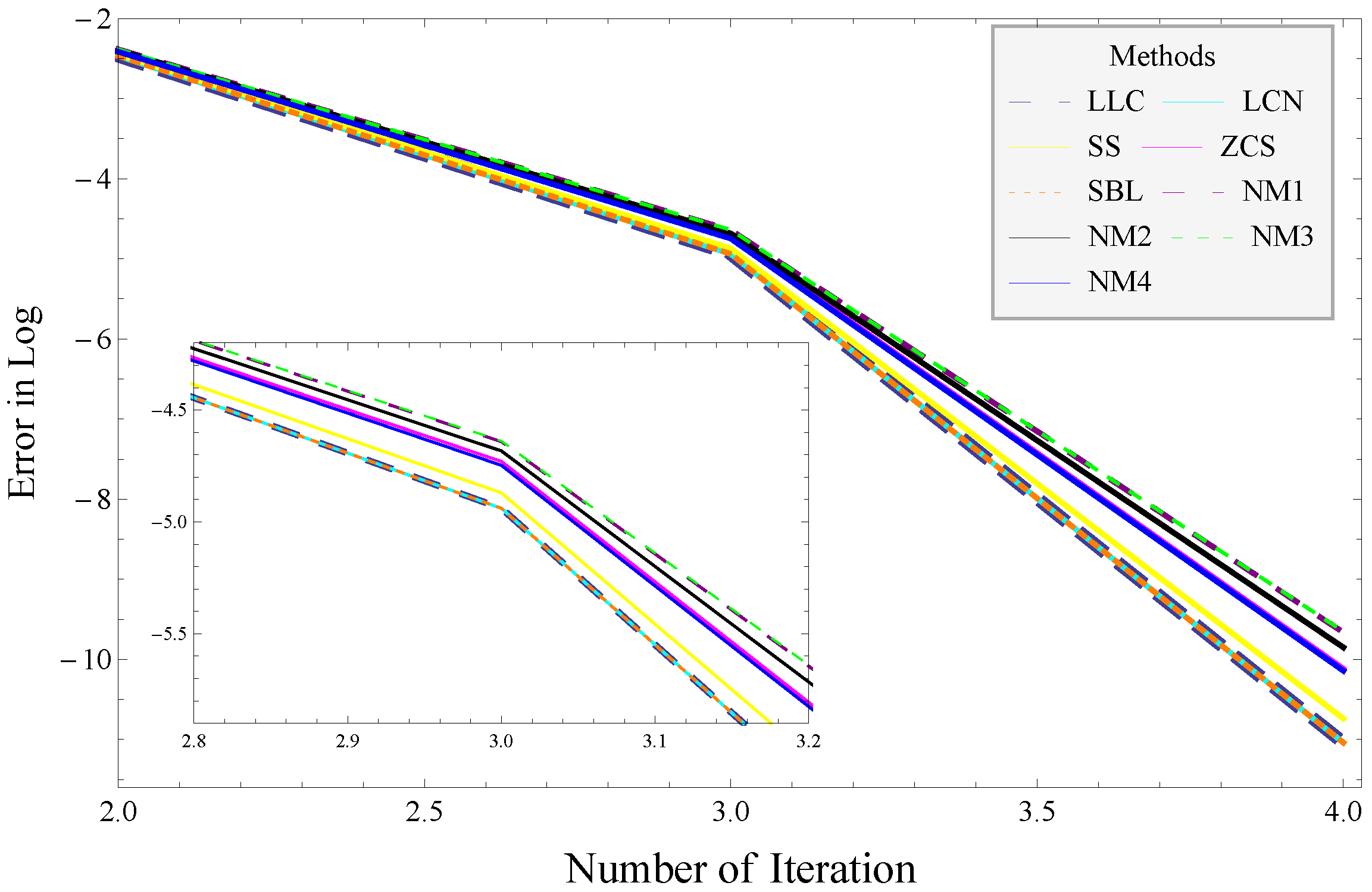
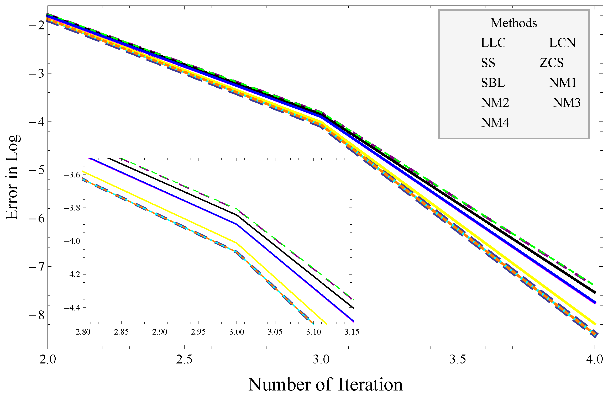
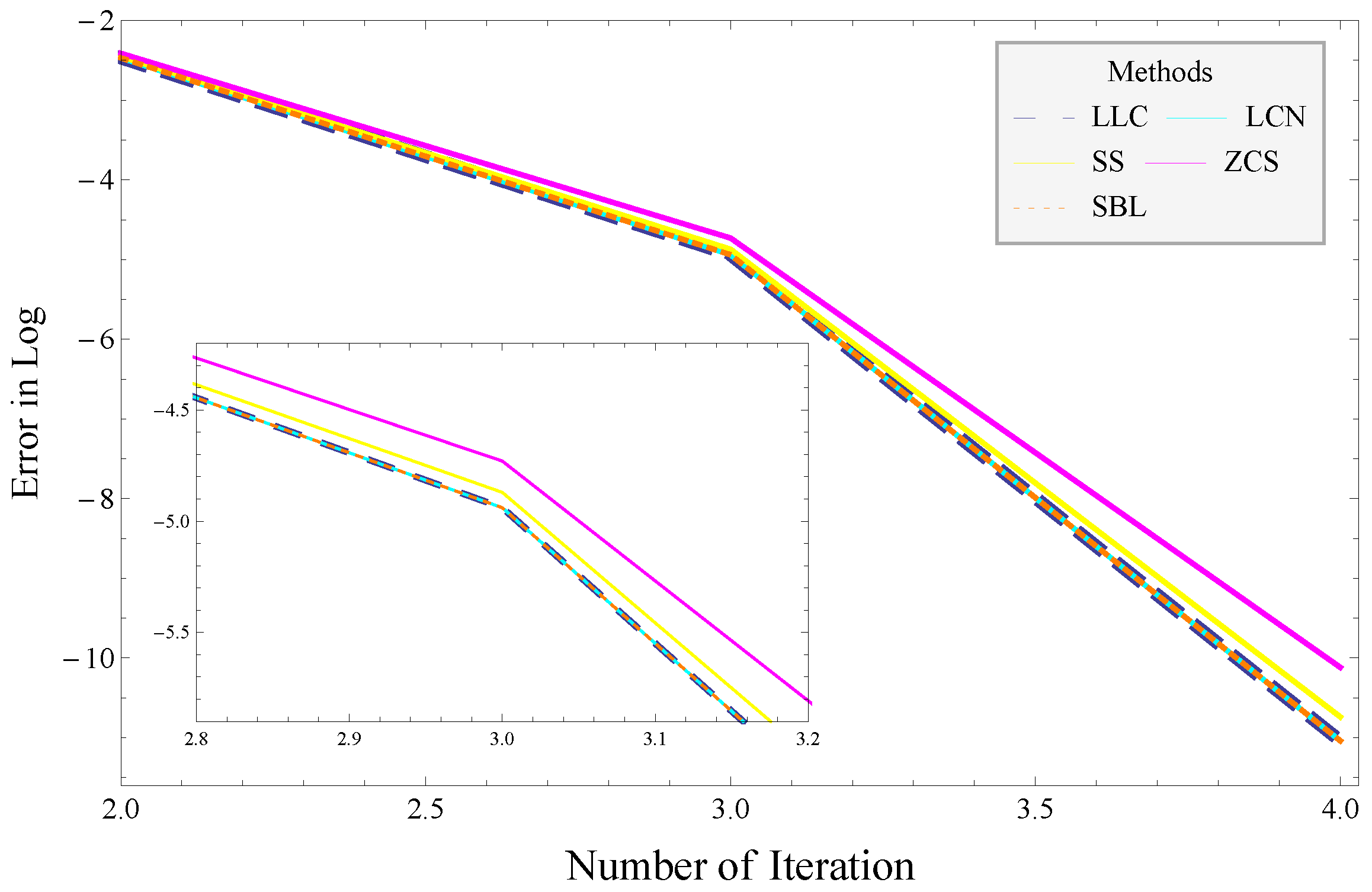
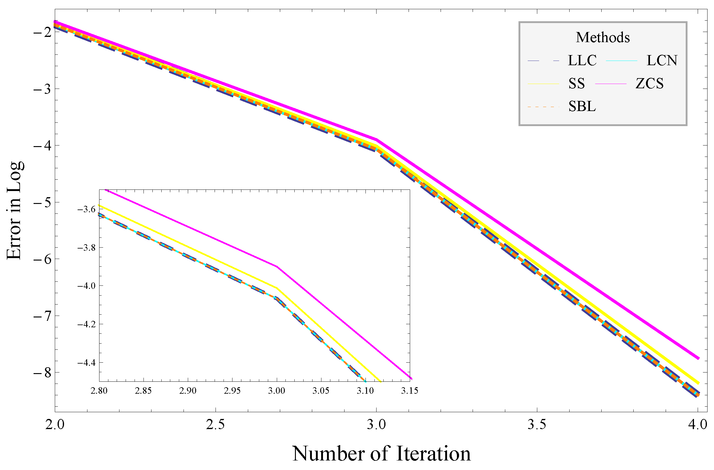
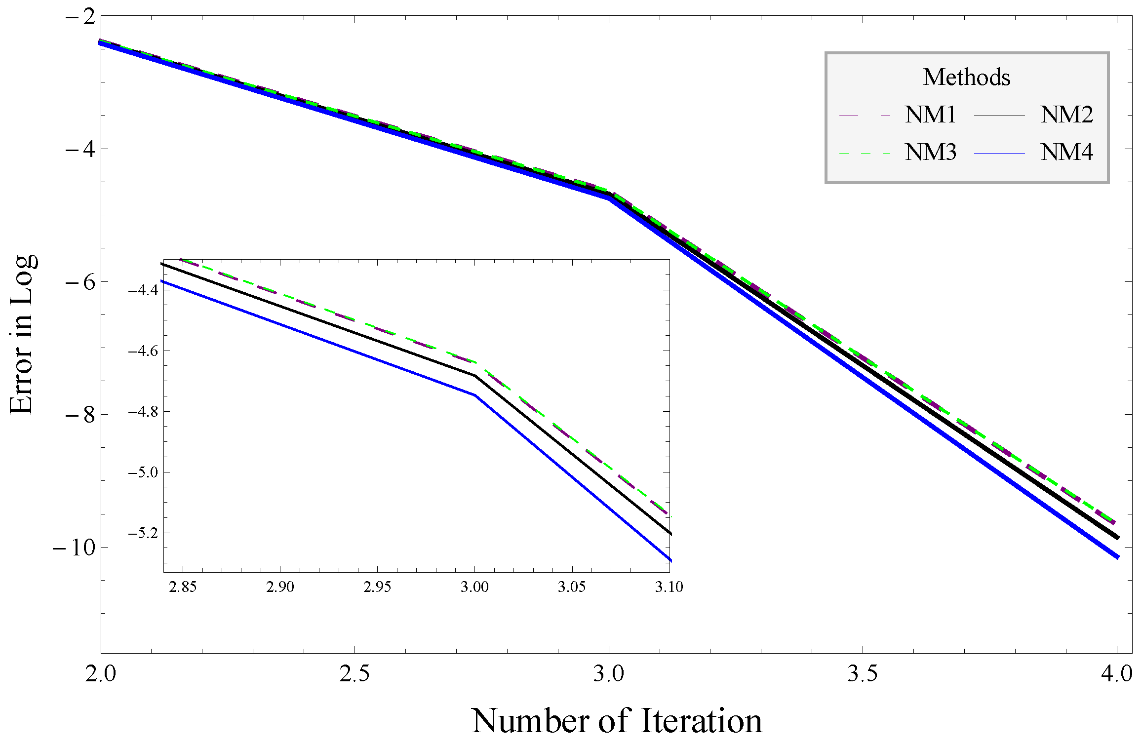
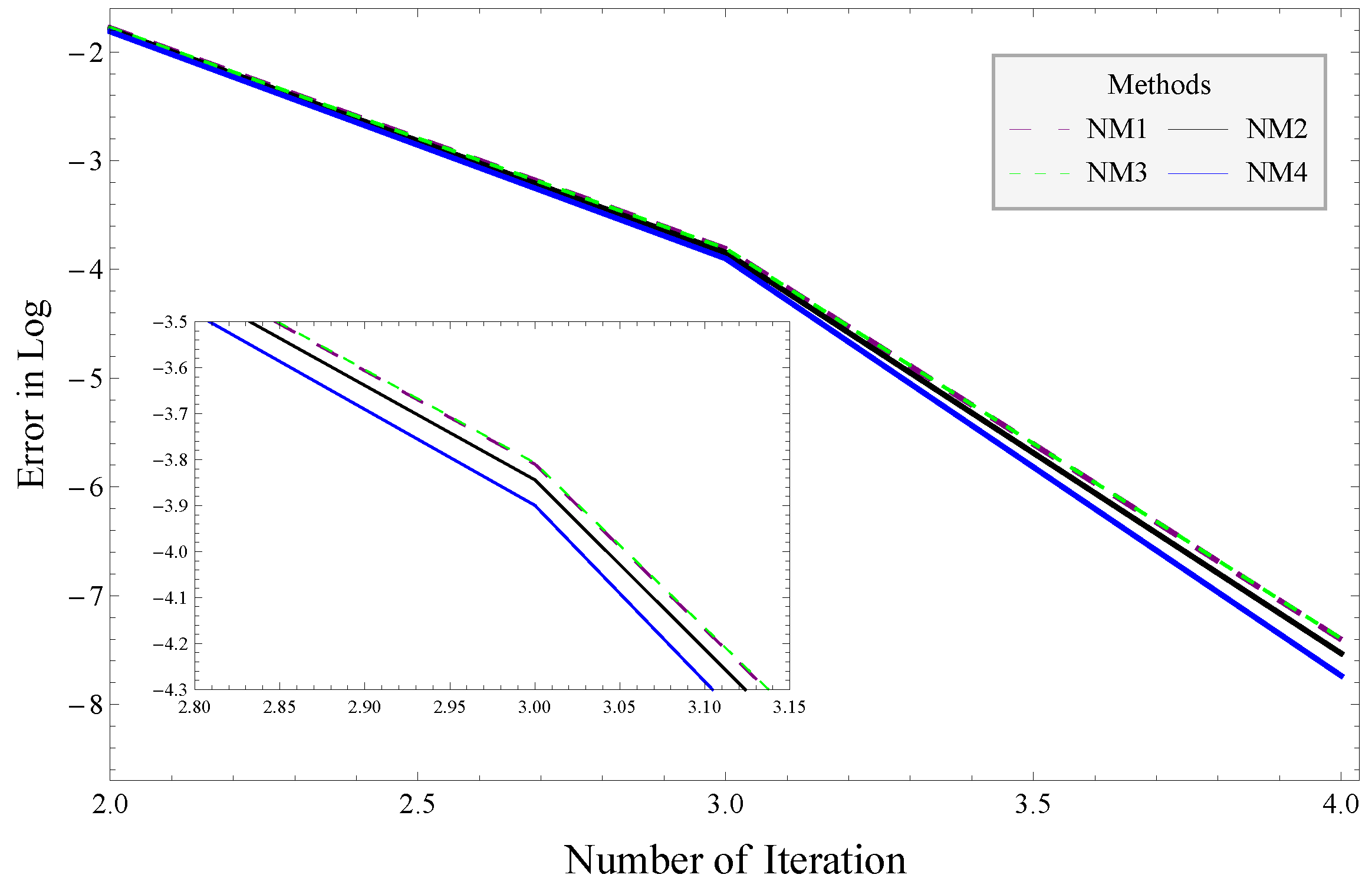
4. Numerical Results

To check the validity and stability of the new algorithms, we have considered some real-life problems which prove the results that we have shown in the preceding sections. Moreover, new algorithms are compared with existing fourth order algorithms that use derivatives in the formulas. For example, the following five schemes are taken for comparison:

Li et al. method [21] (LLC):

$$\begin{array}{cc}\hfill z_p=& t_p-\frac{2m}{m+2}\frac{\chi \left(t_p\right)}{{\chi }^{\prime }\left(t_p\right)},\hfill \\ \hfill t_{p+1}=& t_p-\frac{m(m-2){\left(\frac{m}{m+2}\right)}^{-m}{\chi }^{\prime }\left(z_p\right)-m^2{\chi }^{\prime }\left(t_p\right)}{{\chi }^{\prime }\left(t_p\right)-{\left(\frac{m}{m+2}\right)}^{-m}{\chi }^{\prime }\left(z_p\right)}\frac{\chi \left(t_p\right)}{2{\chi }^{\prime }\left(t_p\right)}.\hfill \end{array}$$

Li et al. method [22] (LCN):

$$\begin{array}{cc}\hfill z_p=& t_p-\frac{2m}{m+2}\frac{\chi \left(t_p\right)}{{\chi }^{\prime }\left(t_p\right)},\hfill \\ \hfill t_{p+1}=& t_p-{\alpha }_1\frac{\chi \left(t_p\right)}{{\chi }^{\prime }\left(z_p\right)}-\frac{\chi \left(t_p\right)}{{\alpha }_2{\chi }^{\prime }\left(t_p\right)+{\alpha }_3{\chi }^{\prime }\left(z_p\right)},\hfill \end{array}$$

where

$$\begin{array}{cc}\hfill {\alpha }_1=& -\frac{1}{2}\frac{{\left(\frac{m}{m+2}\right)}^{m}m(m^4+4m^3-16m-16)}{m^3-4m+8},\hfill \\ \hfill {\alpha }_2=& -\frac{{(8-4m+m^3)}^2}{m(m^2+2m-4)(m^4+4m^3-4m^2-16m+16)},\hfill \\ \hfill {\alpha }_3=& \frac{m^2(m^3-4m+8)}{{\left(\frac{m}{m+2}\right)}^m(m^2+2m-4)(m^4+4m^3-4m^2-16m+16)}.\hfill \end{array}$$

Sharma-Sharma method [23] (SS):

$$\begin{array}{cc}\hfill z_p=& t_p-\frac{2m}{m+2}\frac{\chi \left(t_p\right)}{{\chi }^{\prime }\left(t_p\right)},\hfill \\ \hfill t_{p+1}=& t_p-\frac{m}{8}[(m^3-4m+8)-{(2+m)}^2{\left(\frac{m}{m+2}\right)}^m\frac{{\chi }^{\prime }\left(t_p\right)}{{\chi }^{\prime }\left(z_p\right)}\hfill \\ \hfill & \times \left(2(m-1)-(2+m){\left(\frac{m}{m+2}\right)}^m\frac{{\chi }^{\prime }\left(t_p\right)}{{\chi }^{\prime }\left(z_p\right)}\right)]\frac{\chi \left(t_p\right)}{{\chi }^{\prime }\left(t_p\right)}.\hfill \end{array}$$

Zhou et al. method [24] (ZCS):

$$\begin{array}{cc}\hfill z_p=& t_p-\frac{2m}{m+2}\frac{\chi \left(t_p\right)}{{\chi }^{\prime }\left(t_p\right)},\hfill \\ \hfill t_{p+1}=& t_p-\frac{m}{8}[m^3{\left(\frac{m+2}{m}\right)}^{2m}{\left(\frac{{\chi }^{\prime }\left(z_p\right)}{{\chi }^{\prime }\left(t_p\right)}\right)}^2-2m^2(3+m){\left(\frac{2+m}{m}\right)}^m\frac{{\chi }^{\prime }\left(z_p\right)}{{\chi }^{\prime }\left(t_p\right)}\hfill \\ \hfill & +(m^3+6m^2+8m+8)]\frac{\chi \left(t_p\right)}{{\chi }^{\prime }\left(t_p\right)}.\hfill \end{array}$$

Soleymani et al. method [25] (SBL):

$$\begin{array}{cc}\hfill z_p=& t_p-\frac{2m}{m+2}\frac{\chi \left(t_p\right)}{{\chi }^{\prime }\left(t_p\right)},\hfill \\ \hfill t_{p+1}=& t_p-\frac{{\chi }^{\prime }\left(z_p\right)\chi \left(t_p\right)}{q_1{\left({\chi }^{\prime }\left(z_p\right)\right)}^2+q_2{\chi }^{\prime }\left(z_p\right){\chi }^{\prime }\left(t_p\right)+q_3{\left({\chi }^{\prime }\left(t_p\right)\right)}^2},\hfill \end{array}$$

where

$$\begin{array}{cc}\hfill q_1=& \frac{1}{16}{m}^{3-m}{(m+2)}^m,\hfill \\ \hfill q_2=& \frac{8-m(m+2)(m^2-2)}{8m},\hfill \\ \hfill q_3=& \frac{1}{16}(m-2)m^{m-1}{(m+2)}^{3-m}.\hfill \end{array}$$

The numerical work of this study is performed in software Mathematica [50]. In computation, we use the value $0.01$ for parameter $\beta$. The idea for taking small value is clear from the Traub-Steffensen formula (1), developed by replacing the derivative in the Newton formula (2) with the divided difference, as shown above in the Introduction section, since small values of $\beta$ will give a more accurate approximation. The results displayed in Table 1, Table 2, Table 3, Table 4 and Table 5 are performed in respect of the following:

(i)

The number of iterations $(p+1)$ taken by the algorithms and the satisfaction of the stopping criterion $|t_{p+1}-t_p|+|\chi \left(t_{p+1}\right)|<{10}^{-100}$.

(ii)

The first three iterations’ error $|t_{p+1}-t_p|$.

(iii)

The calculated convergence order (CCO).

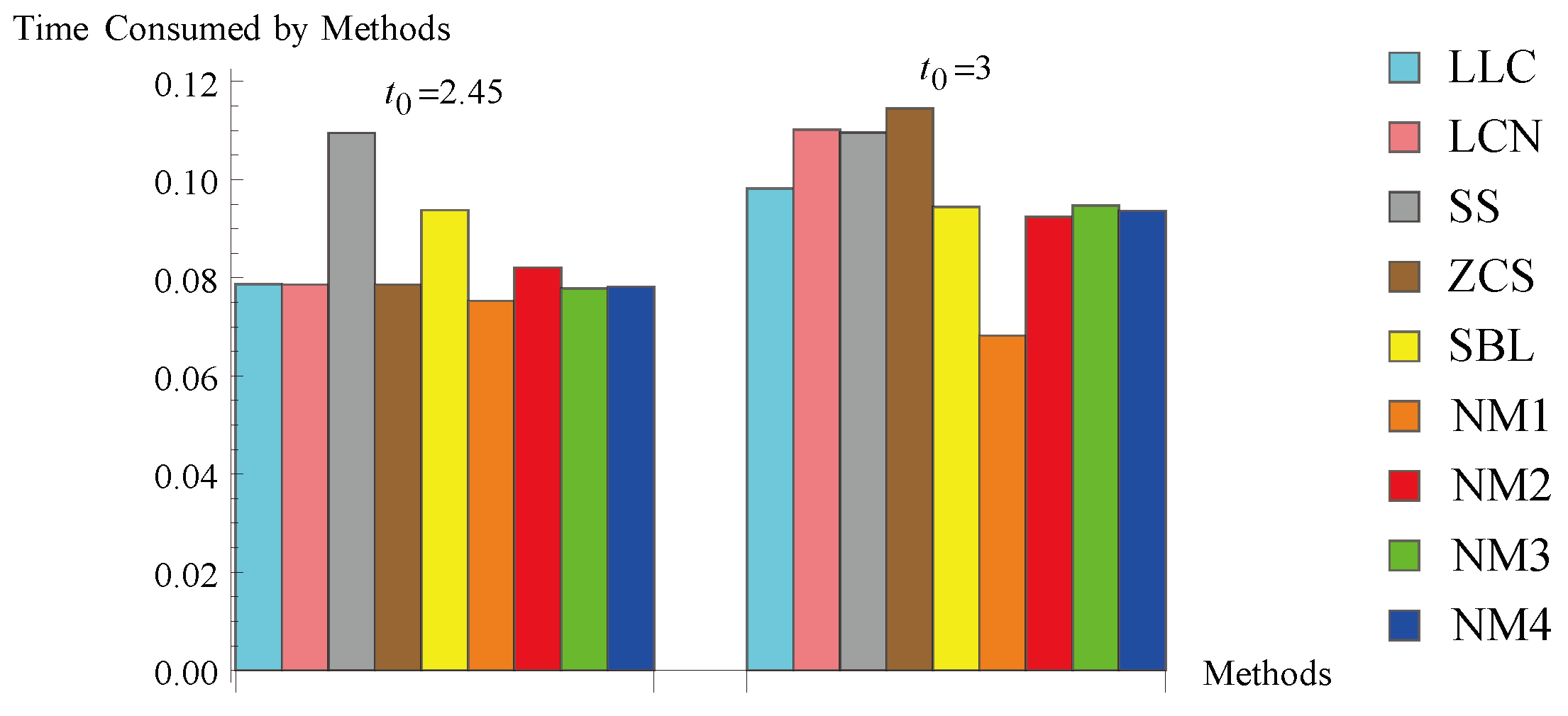
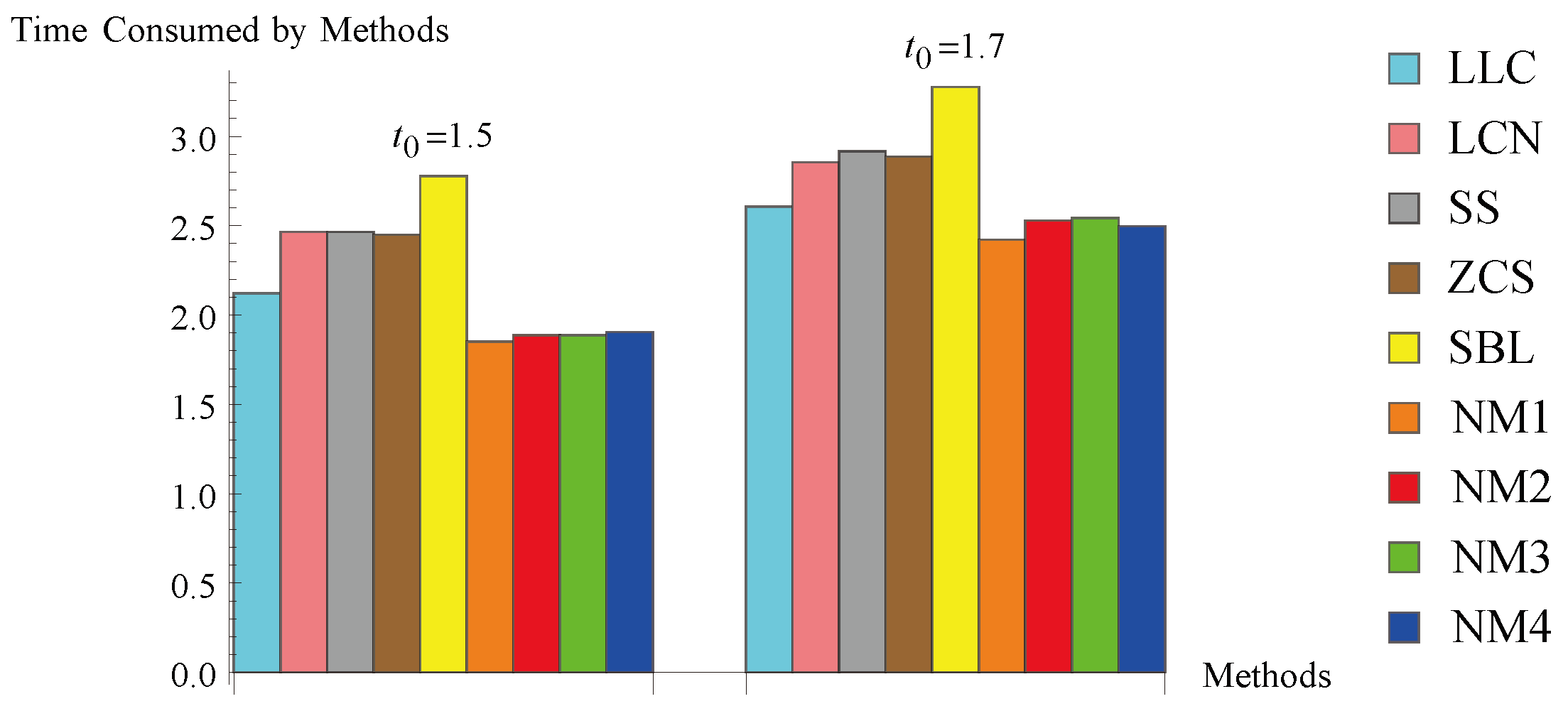
(iv)

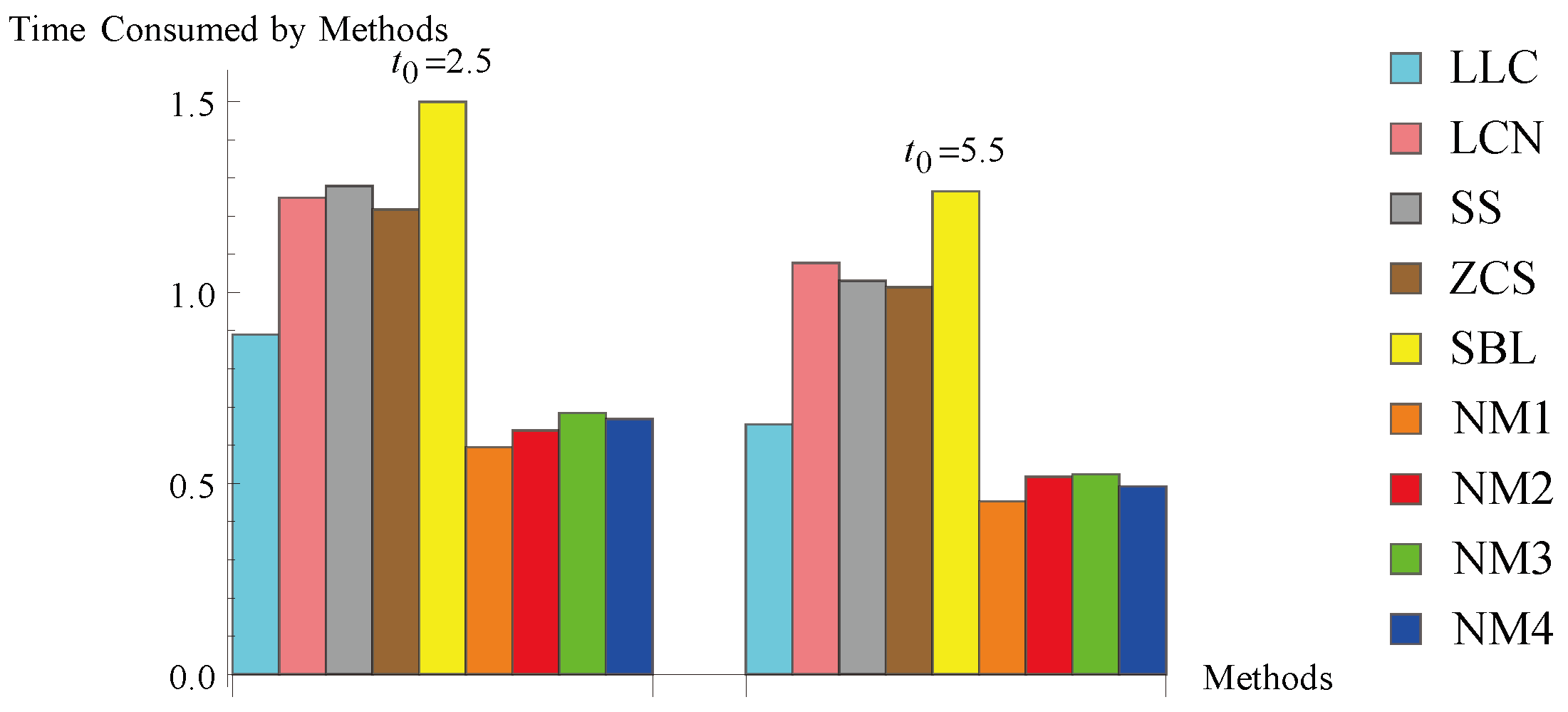
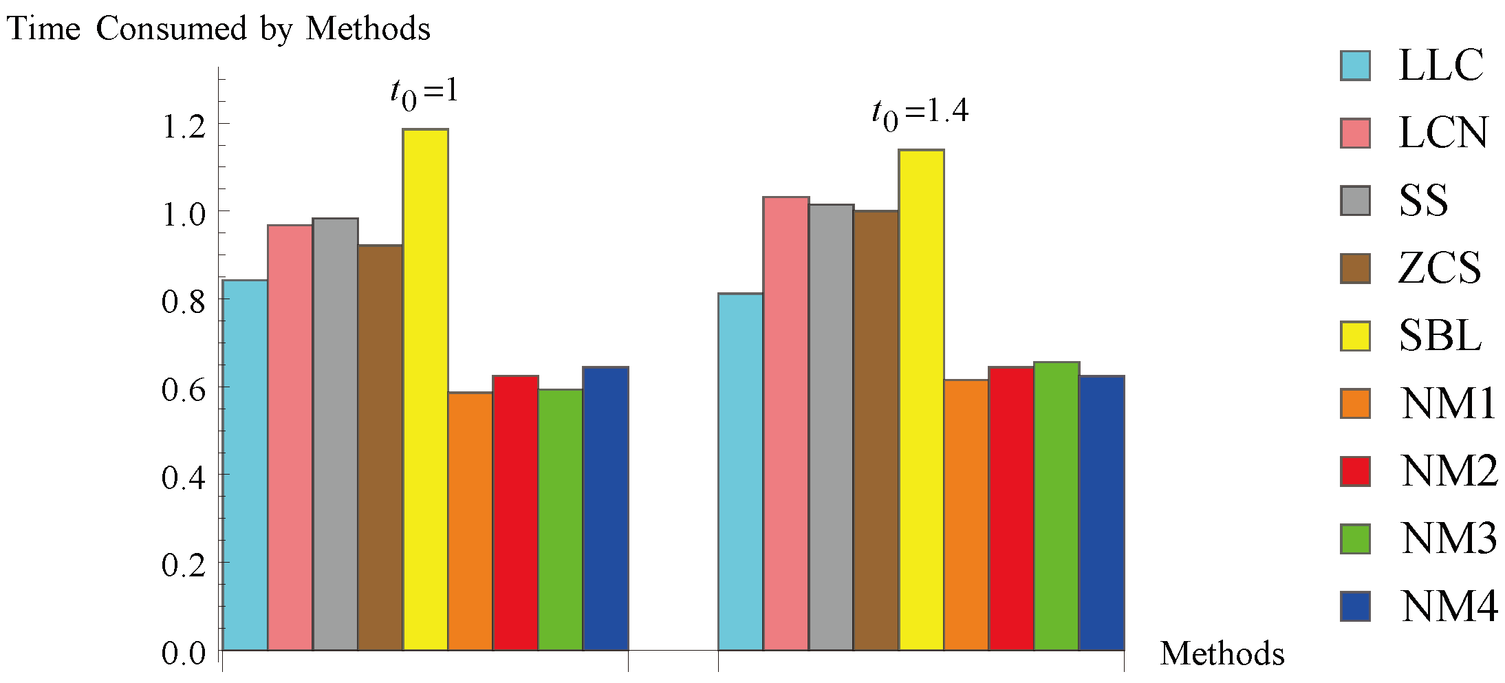
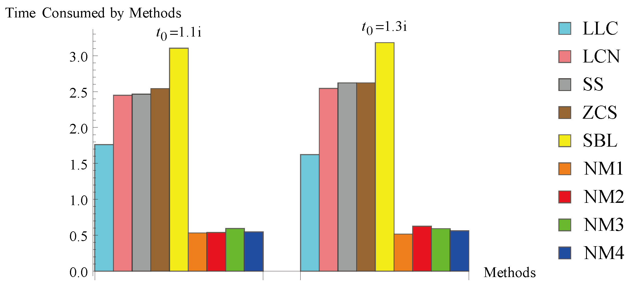
The total time (in seconds) consumed by the algorithms.

To calculate the convergence order (CCO), we use the formula (see [51])

$$\mathrm{CCO}=\frac{log|e_{p+2}/e_{p+1}|}{log|e_{p+1}/e_p|},\mathrm{for}\mathrm{each}p=1,2,\dots ,$$

(32)

where $e_p=t_p-\overline{\mathrm{a}}.$

Let us consider the following problems for the testing:

Problem 1: The Van der Waals equation for a gas [42,52] is given by

$$\left(P+\frac{a_1{n}^2}{V^2}\right)(V-n{a}_2)=n\mathrm{R}T$$

(33)

where, R: universal gas constant, T: temperature, P: pressure, V: volume, n: number of moles, $a_1$, $a_2$: variables with values depending on the gas. To calculate the volume V, we can write (33) as

$$P{V}^3-(n{a}_{2}P+n\mathrm{R}T)V^2+a_1{n}^{2}V-a_1{a}_2{n}^2=0.$$

(34)

One can find values of n, P, T, $a_1$ and $a_2$ of a particular gas [52] such that Equation (34) has three roots. So, by using a specific set of values, we have

$${\chi }_1\left(t\right)=t^3-5.22t^2+9.0825t-5.2675,$$

that has three roots $\overline{a}=1.72,1.75,1.75$. So, our desired root is $\overline{a}=1.75$ with $m=2$. The methods are tested for two initial guesses $t_0=2.45,3$. Computed results are given in Table 6. Figure 1 and Figure 2 represent the graph of the errors committed by methods as iteration proceeds for ${\chi }_1\left(t\right)$ at $t_0=2.45$ and $t_0=3$, respectively. However, some graphs overlap each other. So, to make it more clear, we further draw the graphs in Figure 3 and Figure 4 for the following methods: LLC, LCN, SS, ZCS, SBL, and Figure 5 and Figure 6 for the methods: NM1, NM2, NM3 and NM4. To make the pictures more clear, the bending portion of the lines is shown in sub-figures within the Figure 1, Figure 2, Figure 3, Figure 4, Figure 5 and Figure 6. It can be observed from the graphs that newly proposed methods are good competitors to existing Newton-like methods. Figure 1, Figure 2, Figure 3, Figure 4, Figure 5 and Figure 6 are drawn using the Mathematica software. These figures are the geometrical representation of the errors shown in columns 3, 4, and 5 of Table 6 that help us visualize methods’ behavior for different initial guesses.

Table 1. Numerical problems 2–5.

Problem	Root	Multiplicity	Initial Guess	Results’ Table
2: Isentropic supersonic flow problem [53]
${\chi }_2\left(t\right)=[{tan}^{-1}\left(\frac{\sqrt{5}}{2}\right)-{tan}^{-1}\left(\sqrt{t^2-1}\right)$
$+\sqrt{6}\left({tan}^{-1}\left(\sqrt{\frac{t^2-1}{6}}\right)-{tan}^{-1}\left(\frac{1}{2}\sqrt{\frac{5}{6}}\right)\right)-\frac{11}{63}{]}^3$	1.8411…	3	1.5 & 1.7	Table 2
3: Planck law of radiation problem [54]
${\chi }_3\left(t\right)={\left(e^{-t}-1+\frac{t}{5}\right)}^4$	4.9651…	4	2.5 & 5.5	Table 3
4: Kepler’s problem [49]
${\chi }_4\left(t\right)={\left(t-\frac{1}{4}\sin \left(t\right)-\frac{\pi }{5}\right)}^5$	0.8093…	5	1 & 1.4	Table 4
5: Complex root problem
${\chi }_5\left(t\right)=t(t^2+1)(2e^{t^2+1}+t^2-1){\cos \mathrm{h}}^4\left(\frac{\pi t}{2}\right)$	i	6	1.1 i & 1.3 i	Table 5

Table 1. Numerical problems 2–5.

Problem	Root	Multiplicity	Initial Guess	Results’ Table
2: Isentropic supersonic flow problem [53]
${\chi }_2\left(t\right)=[{tan}^{-1}\left(\frac{\sqrt{5}}{2}\right)-{tan}^{-1}\left(\sqrt{t^2-1}\right)$
$+\sqrt{6}\left({tan}^{-1}\left(\sqrt{\frac{t^2-1}{6}}\right)-{tan}^{-1}\left(\frac{1}{2}\sqrt{\frac{5}{6}}\right)\right)-\frac{11}{63}{]}^3$	1.8411…	3	1.5 & 1.7	Table 2
3: Planck law of radiation problem [54]
${\chi }_3\left(t\right)={\left(e^{-t}-1+\frac{t}{5}\right)}^4$	4.9651…	4	2.5 & 5.5	Table 3
4: Kepler’s problem [49]
${\chi }_4\left(t\right)={\left(t-\frac{1}{4}\sin \left(t\right)-\frac{\pi }{5}\right)}^5$	0.8093…	5	1 & 1.4	Table 4
5: Complex root problem
${\chi }_5\left(t\right)=t(t^2+1)(2e^{t^2+1}+t^2-1){\cos \mathrm{h}}^4\left(\frac{\pi t}{2}\right)$	i	6	1.1 i & 1.3 i	Table 5

Table 2. Numerical results of methods for problem 2.

Methods	$\mathit{p}+1$	$|{\mathit{t}}_2-{\mathit{t}}_1|$	$|{\mathit{t}}_3-{\mathit{t}}_2|$	$|{\mathit{t}}_4-{\mathit{t}}_3|$	CCO	CPU-Time
$t_0=1.5$
LLC	4	$8.19\times {10}^{-4}$	$2.64\times {10}^{-15}$	$2.87\times {10}^{-61}$	4	2.1224
LCN	4	$8.19\times {10}^{-4}$	$2.61\times {10}^{-15}$	$2.73\times {10}^{-61}$	4	2.4660
SS	4	$8.19\times {10}^{-4}$	$2.55\times {10}^{-15}$	$2.44\times {10}^{-61}$	4	2.4653
ZCS	4	$8.19\times {10}^{-4}$	$2.40\times {10}^{-15}$	$1.79\times {10}^{-61}$	4	2.4492
SBL	4	$8.19\times {10}^{-4}$	$2.53\times {10}^{-15}$	$2.34\times {10}^{-61}$	4	2.7765
NM1	4	$2.76\times {10}^{-5}$	$8.29\times {10}^{-21}$	$6.75\times {10}^{-83}$	4	1.8522
NM2	4	$2.76\times {10}^{-5}$	$8.05\times {10}^{-21}$	$5.83\times {10}^{-83}$	4	1.8878
NM3	4	$2.76\times {10}^{-5}$	$8.29\times {10}^{-21}$	$6.75\times {10}^{-83}$	4	1.8867
NM4	4	$2.76\times {10}^{-5}$	$7.69\times {10}^{-21}$	$4.65\times {10}^{-83}$	4	1.9042
$t_0=1.7$
LLC	4	$7.01\times {10}^{-6}$	$1.42\times {10}^{-23}$	$2.43\times {10}^{-94}$	4	2.6054
LCN	4	$7.00\times {10}^{-6}$	$1.40\times {10}^{-23}$	$2.27\times {10}^{-94}$	4	2.8556
SS	4	$6.98\times {10}^{-6}$	$1.36\times {10}^{-23}$	$1.93\times {10}^{-94}$	4	2.9173
ZCS	4	$6.93\times {10}^{-6}$	$1.24\times {10}^{-23}$	$1.27\times {10}^{-94}$	4	2.8868
SBL	4	$6.97\times {10}^{-6}$	$1.34\times {10}^{-23}$	$1.82\times {10}^{-94}$	4	3.2764
NM1	4	$4.04\times {10}^{-6}$	$3.82\times {10}^{-24}$	$3.04\times {10}^{-96}$	4	2.4214
NM2	4	$3.99\times {10}^{-6}$	$3.51\times {10}^{-24}$	$2.11\times {10}^{-96}$	4	2.5285
NM3	4	$4.04\times {10}^{-6}$	$3.82\times {10}^{-24}$	$3.04\times {10}^{-96}$	4	2.5432
NM4	4	$3.90\times {10}^{-6}$	$3.09\times {10}^{-24}$	$1.21\times {10}^{-96}$	4	2.4967

Table 2. Numerical results of methods for problem 2.

Methods	$\mathit{p}+1$	$|{\mathit{t}}_2-{\mathit{t}}_1|$	$|{\mathit{t}}_3-{\mathit{t}}_2|$	$|{\mathit{t}}_4-{\mathit{t}}_3|$	CCO	CPU-Time
$t_0=1.5$
LLC	4	$8.19\times {10}^{-4}$	$2.64\times {10}^{-15}$	$2.87\times {10}^{-61}$	4	2.1224
LCN	4	$8.19\times {10}^{-4}$	$2.61\times {10}^{-15}$	$2.73\times {10}^{-61}$	4	2.4660
SS	4	$8.19\times {10}^{-4}$	$2.55\times {10}^{-15}$	$2.44\times {10}^{-61}$	4	2.4653
ZCS	4	$8.19\times {10}^{-4}$	$2.40\times {10}^{-15}$	$1.79\times {10}^{-61}$	4	2.4492
SBL	4	$8.19\times {10}^{-4}$	$2.53\times {10}^{-15}$	$2.34\times {10}^{-61}$	4	2.7765
NM1	4	$2.76\times {10}^{-5}$	$8.29\times {10}^{-21}$	$6.75\times {10}^{-83}$	4	1.8522
NM2	4	$2.76\times {10}^{-5}$	$8.05\times {10}^{-21}$	$5.83\times {10}^{-83}$	4	1.8878
NM3	4	$2.76\times {10}^{-5}$	$8.29\times {10}^{-21}$	$6.75\times {10}^{-83}$	4	1.8867
NM4	4	$2.76\times {10}^{-5}$	$7.69\times {10}^{-21}$	$4.65\times {10}^{-83}$	4	1.9042
$t_0=1.7$
LLC	4	$7.01\times {10}^{-6}$	$1.42\times {10}^{-23}$	$2.43\times {10}^{-94}$	4	2.6054
LCN	4	$7.00\times {10}^{-6}$	$1.40\times {10}^{-23}$	$2.27\times {10}^{-94}$	4	2.8556
SS	4	$6.98\times {10}^{-6}$	$1.36\times {10}^{-23}$	$1.93\times {10}^{-94}$	4	2.9173
ZCS	4	$6.93\times {10}^{-6}$	$1.24\times {10}^{-23}$	$1.27\times {10}^{-94}$	4	2.8868
SBL	4	$6.97\times {10}^{-6}$	$1.34\times {10}^{-23}$	$1.82\times {10}^{-94}$	4	3.2764
NM1	4	$4.04\times {10}^{-6}$	$3.82\times {10}^{-24}$	$3.04\times {10}^{-96}$	4	2.4214
NM2	4	$3.99\times {10}^{-6}$	$3.51\times {10}^{-24}$	$2.11\times {10}^{-96}$	4	2.5285
NM3	4	$4.04\times {10}^{-6}$	$3.82\times {10}^{-24}$	$3.04\times {10}^{-96}$	4	2.5432
NM4	4	$3.90\times {10}^{-6}$	$3.09\times {10}^{-24}$	$1.21\times {10}^{-96}$	4	2.4967

Table 3. Numerical results of methods for problem 3.

Methods	$\mathit{p}+1$	$|{\mathit{t}}_2-{\mathit{t}}_1|$	$|{\mathit{t}}_3-{\mathit{t}}_2|$	$|{\mathit{t}}_4-{\mathit{t}}_3|$	CCO	CPU-Time
$t_0=2.5$
LLC	5	$2.94$	$8.02\times {10}^{-3}$	$4.02\times {10}^{-12}$	4	0.8893
LCN	5	$2.93$	$7.94\times {10}^{-3}$	$3.86\times {10}^{-12}$	4	1.2483
SS	5	$2.90$	$7.78\times {10}^{-3}$	$3.56\times {10}^{-12}$	4	1.2791
ZCS	5	$2.86$	$7.55\times {10}^{-3}$	$3.16\times {10}^{-12}$	4	1.2172
SBL	5	$2.77$	$7.03\times {10}^{-3}$	$2.37\times {10}^{-12}$	4	1.4986
NM1	5	$4.68$	$9.00\times {10}^{-4}$	$9.07\times {10}^{-17}$	4	0.5946
NM2	5	$4.58$	$8.65\times {10}^{-4}$	$7.67\times {10}^{-17}$	4	0.6385
NM3	5	$4.66$	$8.94\times {10}^{-4}$	$8.82\times {10}^{-17}$	4	0.6843
NM4	5	$4.87$	$9.62\times {10}^{-4}$	$1.15\times {10}^{-16}$	4	0.6682
$t_0=5.5$
LLC	4	$4.91\times {10}^{-5}$	$5.70\times {10}^{-21}$	$1.03\times {10}^{-84}$	4	0.6545
LCN	4	$4.91\times {10}^{-5}$	$5.70\times {10}^{-21}$	$1.03\times {10}^{-84}$	4	1.0772
SS	4	$4.92\times {10}^{-5}$	$5.71\times {10}^{-21}$	$1.04\times {10}^{-84}$	4	1.0301
ZCS	4	$4.92\times {10}^{-5}$	$5.72\times {10}^{-21}$	$1.05\times {10}^{-84}$	4	1.0142
SBL	4	$4.92\times {10}^{-5}$	$5.73\times {10}^{-21}$	$1.06\times {10}^{-84}$	4	1.2646
NM1	3	$5.57\times {10}^{-6}$	$1.33\times {10}^{-25}$	0	4	0.4534
NM2	3	$5.53\times {10}^{-6}$	$1.28\times {10}^{-25}$	0	4	0.5173
NM3	3	$5.57\times {10}^{-6}$	$1.33\times {10}^{-25}$	0	4	0.5238
NM4	3	$5.47\times {10}^{-6}$	$1.21\times {10}^{-25}$	0	4	0.4923

Table 3. Numerical results of methods for problem 3.

Methods	$\mathit{p}+1$	$|{\mathit{t}}_2-{\mathit{t}}_1|$	$|{\mathit{t}}_3-{\mathit{t}}_2|$	$|{\mathit{t}}_4-{\mathit{t}}_3|$	CCO	CPU-Time
$t_0=2.5$
LLC	5	$2.94$	$8.02\times {10}^{-3}$	$4.02\times {10}^{-12}$	4	0.8893
LCN	5	$2.93$	$7.94\times {10}^{-3}$	$3.86\times {10}^{-12}$	4	1.2483
SS	5	$2.90$	$7.78\times {10}^{-3}$	$3.56\times {10}^{-12}$	4	1.2791
ZCS	5	$2.86$	$7.55\times {10}^{-3}$	$3.16\times {10}^{-12}$	4	1.2172
SBL	5	$2.77$	$7.03\times {10}^{-3}$	$2.37\times {10}^{-12}$	4	1.4986
NM1	5	$4.68$	$9.00\times {10}^{-4}$	$9.07\times {10}^{-17}$	4	0.5946
NM2	5	$4.58$	$8.65\times {10}^{-4}$	$7.67\times {10}^{-17}$	4	0.6385
NM3	5	$4.66$	$8.94\times {10}^{-4}$	$8.82\times {10}^{-17}$	4	0.6843
NM4	5	$4.87$	$9.62\times {10}^{-4}$	$1.15\times {10}^{-16}$	4	0.6682
$t_0=5.5$
LLC	4	$4.91\times {10}^{-5}$	$5.70\times {10}^{-21}$	$1.03\times {10}^{-84}$	4	0.6545
LCN	4	$4.91\times {10}^{-5}$	$5.70\times {10}^{-21}$	$1.03\times {10}^{-84}$	4	1.0772
SS	4	$4.92\times {10}^{-5}$	$5.71\times {10}^{-21}$	$1.04\times {10}^{-84}$	4	1.0301
ZCS	4	$4.92\times {10}^{-5}$	$5.72\times {10}^{-21}$	$1.05\times {10}^{-84}$	4	1.0142
SBL	4	$4.92\times {10}^{-5}$	$5.73\times {10}^{-21}$	$1.06\times {10}^{-84}$	4	1.2646
NM1	3	$5.57\times {10}^{-6}$	$1.33\times {10}^{-25}$	0	4	0.4534
NM2	3	$5.53\times {10}^{-6}$	$1.28\times {10}^{-25}$	0	4	0.5173
NM3	3	$5.57\times {10}^{-6}$	$1.33\times {10}^{-25}$	0	4	0.5238
NM4	3	$5.47\times {10}^{-6}$	$1.21\times {10}^{-25}$	0	4	0.4923

Table 4. Numerical results of methods for problem 4.

Methods	$\mathit{p}+1$	$|{\mathit{t}}_2-{\mathit{t}}_1|$	$|{\mathit{t}}_3-{\mathit{t}}_2|$	$|{\mathit{t}}_4-{\mathit{t}}_3|$	CCO	CPU-Time
$t_0=1$
LLC	4	$1.24\times {10}^{-5}$	$2.79\times {10}^{-22}$	$7.12\times {10}^{-89}$	4	0.8422
LCN	4	$1.24\times {10}^{-5}$	$2.74\times {10}^{-22}$	$6.60\times {10}^{-89}$	4	0.9675
SS	4	$1.23\times {10}^{-5}$	$2.61\times {10}^{-22}$	$5.40\times {10}^{-89}$	4	0.9833
ZCS	4	$1.21\times {10}^{-5}$	$2.45\times {10}^{-22}$	$4.14\times {10}^{-89}$	4	0.9215
SBL	4	$1.15\times {10}^{-5}$	$1.94\times {10}^{-22}$	$1.57\times {10}^{-89}$	4	1.1863
NM1	4	$5.37\times {10}^{-6}$	$2.28\times {10}^{-24}$	$7.42\times {10}^{-98}$	4	0.5865
NM2	4	$4.99\times {10}^{-6}$	$1.54\times {10}^{-24}$	$1.39\times {10}^{-98}$	4	0.6246
NM3	4	$5.38\times {10}^{-6}$	$2.29\times {10}^{-24}$	$7.48\times {10}^{-98}$	4	0.5934
NM4	4	$4.44\times {10}^{-6}$	$8.08\times {10}^{-24}$	$8.88\times {10}^{-100}$	4	0.6440
$t_0=1.4$
LLC	4	$5.08\times {10}^{-4}$	$7.79\times {10}^{-16}$	$4.30\times {10}^{-63}$	4	0.8114
LCN	4	$5.03\times {10}^{-4}$	$7.44\times {10}^{-16}$	$3.56\times {10}^{-63}$	4	1.0320
SS	4	$4.88\times {10}^{-4}$	$6.57\times {10}^{-16}$	$2.15\times {10}^{-63}$	4	1.0146
ZCS	4	$4.69\times {10}^{-4}$	$5.57\times {10}^{-16}$	$1.11\times {10}^{-63}$	4	0.9998
SBL	4	$3.95\times {10}^{-4}$	$2.72\times {10}^{-16}$	$6.10\times {10}^{-65}$	4	1.1393
NM1	4	$6.89\times {10}^{-4}$	$6.17\times {10}^{-16}$	$3.96\times {10}^{-64}$	4	0.6155
NM2	4	$6.56\times {10}^{-4}$	$4.59\times {10}^{-16}$	$1.10\times {10}^{-64}$	4	0.6442
NM3	4	$6.89\times {10}^{-4}$	$6.19\times {10}^{-16}$	$4.03\times {10}^{-64}$	4	0.6561
NM4	4	$6.08\times {10}^{-4}$	$2.85\times {10}^{-16}$	$1.38\times {10}^{-65}$	4	0.6240

Table 4. Numerical results of methods for problem 4.

Methods	$\mathit{p}+1$	$|{\mathit{t}}_2-{\mathit{t}}_1|$	$|{\mathit{t}}_3-{\mathit{t}}_2|$	$|{\mathit{t}}_4-{\mathit{t}}_3|$	CCO	CPU-Time
$t_0=1$
LLC	4	$1.24\times {10}^{-5}$	$2.79\times {10}^{-22}$	$7.12\times {10}^{-89}$	4	0.8422
LCN	4	$1.24\times {10}^{-5}$	$2.74\times {10}^{-22}$	$6.60\times {10}^{-89}$	4	0.9675
SS	4	$1.23\times {10}^{-5}$	$2.61\times {10}^{-22}$	$5.40\times {10}^{-89}$	4	0.9833
ZCS	4	$1.21\times {10}^{-5}$	$2.45\times {10}^{-22}$	$4.14\times {10}^{-89}$	4	0.9215
SBL	4	$1.15\times {10}^{-5}$	$1.94\times {10}^{-22}$	$1.57\times {10}^{-89}$	4	1.1863
NM1	4	$5.37\times {10}^{-6}$	$2.28\times {10}^{-24}$	$7.42\times {10}^{-98}$	4	0.5865
NM2	4	$4.99\times {10}^{-6}$	$1.54\times {10}^{-24}$	$1.39\times {10}^{-98}$	4	0.6246
NM3	4	$5.38\times {10}^{-6}$	$2.29\times {10}^{-24}$	$7.48\times {10}^{-98}$	4	0.5934
NM4	4	$4.44\times {10}^{-6}$	$8.08\times {10}^{-24}$	$8.88\times {10}^{-100}$	4	0.6440
$t_0=1.4$
LLC	4	$5.08\times {10}^{-4}$	$7.79\times {10}^{-16}$	$4.30\times {10}^{-63}$	4	0.8114
LCN	4	$5.03\times {10}^{-4}$	$7.44\times {10}^{-16}$	$3.56\times {10}^{-63}$	4	1.0320
SS	4	$4.88\times {10}^{-4}$	$6.57\times {10}^{-16}$	$2.15\times {10}^{-63}$	4	1.0146
ZCS	4	$4.69\times {10}^{-4}$	$5.57\times {10}^{-16}$	$1.11\times {10}^{-63}$	4	0.9998
SBL	4	$3.95\times {10}^{-4}$	$2.72\times {10}^{-16}$	$6.10\times {10}^{-65}$	4	1.1393
NM1	4	$6.89\times {10}^{-4}$	$6.17\times {10}^{-16}$	$3.96\times {10}^{-64}$	4	0.6155
NM2	4	$6.56\times {10}^{-4}$	$4.59\times {10}^{-16}$	$1.10\times {10}^{-64}$	4	0.6442
NM3	4	$6.89\times {10}^{-4}$	$6.19\times {10}^{-16}$	$4.03\times {10}^{-64}$	4	0.6561
NM4	4	$6.08\times {10}^{-4}$	$2.85\times {10}^{-16}$	$1.38\times {10}^{-65}$	4	0.6240

Table 5. Numerical results of methods for problem 5.

Methods	$\mathit{p}+1$	$|{\mathit{t}}_2-{\mathit{t}}_1|$	$|{\mathit{t}}_3-{\mathit{t}}_2|$	$|{\mathit{t}}_4-{\mathit{t}}_3|$	CCO	CPU-Time
$t_0=1.1i$
LLC	4	$1.75\times {10}^{-5}$	$3.01\times {10}^{-20}$	$2.66\times {10}^{-79}$	4	1.7604
LCN	4	$1.75\times {10}^{-5}$	$3.02\times {10}^{-20}$	$2.68\times {10}^{-79}$	4	2.4491
SS	4	$1.75\times {10}^{-5}$	$3.03\times {10}^{-20}$	$2.73\times {10}^{-79}$	4	2.4653
ZCS	4	$1.75\times {10}^{-5}$	$3.05\times {10}^{-20}$	$2.79\times {10}^{-79}$	4	2.5426
SBL	4	$1.76\times {10}^{-5}$	$3.16\times {10}^{-20}$	$3.28\times {10}^{-79}$	4	3.1042
NM1	4	$6.74\times {10}^{-6}$	$2.93\times {10}^{-22}$	$1.05\times {10}^{-87}$	4	0.5311
NM2	4	$6.69\times {10}^{-6}$	$2.82\times {10}^{-22}$	$8.87\times {10}^{-88}$	4	0.5380
NM3	4	$6.74\times {10}^{-6}$	$2.93\times {10}^{-22}$	$1.05\times {10}^{-87}$	4	0.5935
NM4	4	$6.63\times {10}^{-6}$	$2.66\times {10}^{-22}$	$6.92\times {10}^{-88}$	4	0.5468
$t_0=1.3i$
LLC	4	$1.31\times {10}^{-4}$	$9.41\times {10}^{-17}$	$2.53\times {10}^{-65}$	4	1.6234
LCN	4	$1.31\times {10}^{-4}$	$9.42\times {10}^{-17}$	$2.54\times {10}^{-65}$	4	2.5432
SS	4	$1.31\times {10}^{-4}$	$9.43\times {10}^{-17}$	$2.56\times {10}^{-65}$	4	2.6216
ZCS	4	$1.31\times {10}^{-4}$	$9.45\times {10}^{-17}$	$2.58\times {10}^{-65}$	4	2.6217
SBL	4	$1.31\times {10}^{-4}$	$9.57\times {10}^{-17}$	$2.75\times {10}^{-65}$	4	3.1824
NM1	4	$2.86\times {10}^{-5}$	$9.54\times {10}^{-20}$	$1.18\times {10}^{-77}$	4	0.5162
NM2	4	$2.86\times {10}^{-5}$	$9.41\times {10}^{-20}$	$1.10\times {10}^{-77}$	4	0.6243
NM3	4	$2.86\times {10}^{-5}$	$9.54\times {10}^{-20}$	$1.18\times {10}^{-77}$	4	0.5922
NM4	4	$2.86\times {10}^{-5}$	$9.23\times {10}^{-20}$	$9.98\times {10}^{-78}$	4	0.5610

Table 5. Numerical results of methods for problem 5.

Methods	$\mathit{p}+1$	$|{\mathit{t}}_2-{\mathit{t}}_1|$	$|{\mathit{t}}_3-{\mathit{t}}_2|$	$|{\mathit{t}}_4-{\mathit{t}}_3|$	CCO	CPU-Time
$t_0=1.1i$
LLC	4	$1.75\times {10}^{-5}$	$3.01\times {10}^{-20}$	$2.66\times {10}^{-79}$	4	1.7604
LCN	4	$1.75\times {10}^{-5}$	$3.02\times {10}^{-20}$	$2.68\times {10}^{-79}$	4	2.4491
SS	4	$1.75\times {10}^{-5}$	$3.03\times {10}^{-20}$	$2.73\times {10}^{-79}$	4	2.4653
ZCS	4	$1.75\times {10}^{-5}$	$3.05\times {10}^{-20}$	$2.79\times {10}^{-79}$	4	2.5426
SBL	4	$1.76\times {10}^{-5}$	$3.16\times {10}^{-20}$	$3.28\times {10}^{-79}$	4	3.1042
NM1	4	$6.74\times {10}^{-6}$	$2.93\times {10}^{-22}$	$1.05\times {10}^{-87}$	4	0.5311
NM2	4	$6.69\times {10}^{-6}$	$2.82\times {10}^{-22}$	$8.87\times {10}^{-88}$	4	0.5380
NM3	4	$6.74\times {10}^{-6}$	$2.93\times {10}^{-22}$	$1.05\times {10}^{-87}$	4	0.5935
NM4	4	$6.63\times {10}^{-6}$	$2.66\times {10}^{-22}$	$6.92\times {10}^{-88}$	4	0.5468
$t_0=1.3i$
LLC	4	$1.31\times {10}^{-4}$	$9.41\times {10}^{-17}$	$2.53\times {10}^{-65}$	4	1.6234
LCN	4	$1.31\times {10}^{-4}$	$9.42\times {10}^{-17}$	$2.54\times {10}^{-65}$	4	2.5432
SS	4	$1.31\times {10}^{-4}$	$9.43\times {10}^{-17}$	$2.56\times {10}^{-65}$	4	2.6216
ZCS	4	$1.31\times {10}^{-4}$	$9.45\times {10}^{-17}$	$2.58\times {10}^{-65}$	4	2.6217
SBL	4	$1.31\times {10}^{-4}$	$9.57\times {10}^{-17}$	$2.75\times {10}^{-65}$	4	3.1824
NM1	4	$2.86\times {10}^{-5}$	$9.54\times {10}^{-20}$	$1.18\times {10}^{-77}$	4	0.5162
NM2	4	$2.86\times {10}^{-5}$	$9.41\times {10}^{-20}$	$1.10\times {10}^{-77}$	4	0.6243
NM3	4	$2.86\times {10}^{-5}$	$9.54\times {10}^{-20}$	$1.18\times {10}^{-77}$	4	0.5922
NM4	4	$2.86\times {10}^{-5}$	$9.23\times {10}^{-20}$	$9.98\times {10}^{-78}$	4	0.5610

Table 6. Numerical results of methods for problem 1.

Methods	$\mathit{p}+1$	$|{\mathit{t}}_2-{\mathit{t}}_1|$	$|{\mathit{t}}_3-{\mathit{t}}_2|$	$|{\mathit{t}}_4-{\mathit{t}}_3|$	CCO	CPU-Time
$t_0=2.45$
LLC	6	$8.47\times {10}^{-2}$	$7.16\times {10}^{-3}$	$1.61\times {10}^{-5}$	4	0.0787
LCN	6	$8.47\times {10}^{-2}$	$7.16\times {10}^{-3}$	$1.61\times {10}^{-5}$	4	0.0786
SS	6	$8.63\times {10}^{-2}$	$7.67\times {10}^{-3}$	$2.17\times {10}^{-5}$	4	0.1095
ZCS	6	$8.96\times {10}^{-2}$	$8.83\times {10}^{-3}$	$4.03\times {10}^{-5}$	4	0.0786
SBL	6	$8.47\times {10}^{-2}$	$7.16\times {10}^{-3}$	$1.61\times {10}^{-5}$	4	0.0938
NM1	6	$9.21\times {10}^{-2}$	$9.65\times {10}^{-3}$	$6.36\times {10}^{-5}$	4	0.0753
NM2	6	$9.11\times {10}^{-2}$	$9.25\times {10}^{-3}$	$5.27\times {10}^{-5}$	4	0.0821
NM3	6	$9.22\times {10}^{-2}$	$9.68\times {10}^{-3}$	$6.43\times {10}^{-5}$	4	0.0778
NM4	6	$8.94\times {10}^{-2}$	$8.68\times {10}^{-3}$	$3.94\times {10}^{-5}$	4	0.0782
$t_0=3$
LLC	6	$1.53\times {10}^{-1}$	$1.71\times {10}^{-2}$	$2.26\times {10}^{-4}$	4	0.0982
LCN	6	$1.53\times {10}^{-1}$	$1.71\times {10}^{-2}$	$2.26\times {10}^{-4}$	4	0.1102
SS	6	$1.56\times {10}^{-1}$	$1.81\times {10}^{-2}$	$2.80\times {10}^{-4}$	4	0.1096
ZCS	6	$1.61\times {10}^{-1}$	$2.02\times {10}^{-2}$	$4.32\times {10}^{-4}$	4	0.1145
SBL	6	$1.53\times {10}^{-1}$	$1.71\times {10}^{-2}$	$2.26\times {10}^{-4}$	4	0.0944
NM1	6	$1.69\times {10}^{-1}$	$2.22\times {10}^{-2}$	$6.10\times {10}^{-4}$	4	0.0682
NM2	6	$1.67\times {10}^{-1}$	$2.14\times {10}^{-2}$	$5.37\times {10}^{-4}$	4	0.0924
NM3	6	$1.69\times {10}^{-1}$	$2.22\times {10}^{-2}$	$6.15\times {10}^{-4}$	4	0.0947
NM4	6	$1.63\times {10}^{-1}$	$2.03\times {10}^{-2}$	$4.37\times {10}^{-4}$	4	0.0936

Table 6. Numerical results of methods for problem 1.

Methods	$\mathit{p}+1$	$|{\mathit{t}}_2-{\mathit{t}}_1|$	$|{\mathit{t}}_3-{\mathit{t}}_2|$	$|{\mathit{t}}_4-{\mathit{t}}_3|$	CCO	CPU-Time
$t_0=2.45$
LLC	6	$8.47\times {10}^{-2}$	$7.16\times {10}^{-3}$	$1.61\times {10}^{-5}$	4	0.0787
LCN	6	$8.47\times {10}^{-2}$	$7.16\times {10}^{-3}$	$1.61\times {10}^{-5}$	4	0.0786
SS	6	$8.63\times {10}^{-2}$	$7.67\times {10}^{-3}$	$2.17\times {10}^{-5}$	4	0.1095
ZCS	6	$8.96\times {10}^{-2}$	$8.83\times {10}^{-3}$	$4.03\times {10}^{-5}$	4	0.0786
SBL	6	$8.47\times {10}^{-2}$	$7.16\times {10}^{-3}$	$1.61\times {10}^{-5}$	4	0.0938
NM1	6	$9.21\times {10}^{-2}$	$9.65\times {10}^{-3}$	$6.36\times {10}^{-5}$	4	0.0753
NM2	6	$9.11\times {10}^{-2}$	$9.25\times {10}^{-3}$	$5.27\times {10}^{-5}$	4	0.0821
NM3	6	$9.22\times {10}^{-2}$	$9.68\times {10}^{-3}$	$6.43\times {10}^{-5}$	4	0.0778
NM4	6	$8.94\times {10}^{-2}$	$8.68\times {10}^{-3}$	$3.94\times {10}^{-5}$	4	0.0782
$t_0=3$
LLC	6	$1.53\times {10}^{-1}$	$1.71\times {10}^{-2}$	$2.26\times {10}^{-4}$	4	0.0982
LCN	6	$1.53\times {10}^{-1}$	$1.71\times {10}^{-2}$	$2.26\times {10}^{-4}$	4	0.1102
SS	6	$1.56\times {10}^{-1}$	$1.81\times {10}^{-2}$	$2.80\times {10}^{-4}$	4	0.1096
ZCS	6	$1.61\times {10}^{-1}$	$2.02\times {10}^{-2}$	$4.32\times {10}^{-4}$	4	0.1145
SBL	6	$1.53\times {10}^{-1}$	$1.71\times {10}^{-2}$	$2.26\times {10}^{-4}$	4	0.0944
NM1	6	$1.69\times {10}^{-1}$	$2.22\times {10}^{-2}$	$6.10\times {10}^{-4}$	4	0.0682
NM2	6	$1.67\times {10}^{-1}$	$2.14\times {10}^{-2}$	$5.37\times {10}^{-4}$	4	0.0924
NM3	6	$1.69\times {10}^{-1}$	$2.22\times {10}^{-2}$	$6.15\times {10}^{-4}$	4	0.0947
NM4	6	$1.63\times {10}^{-1}$	$2.03\times {10}^{-2}$	$4.37\times {10}^{-4}$	4	0.0936

The rest of the problems (2–5) are shown in Table 1. This table has five columns: column 1 contains the considered problem, column 2 contains the desired root of the problem, column 3 contains the multiplicity of the root, column 4 displays the initial guess and column 5 shows the table number of the numerical results of the corresponding problem.

We can see from the computed results in Table 6 and Table 2, Table 3, Table 4 and Table 5 that the new methods have good convergence behavior. The increment in precision per iteration, as seen by the numerical results, is the reason for good convergence. This also describes the stable nature of the methods. It is also clear from the computed results that the new methods have better authenticity than those calculated by the existing methods. We display the value $‘0’$ in Table 3 at the stage when the stopping criterion has been satisfied. The calculation of the convergence order in each problem, as shown in the tables, implies verification of the theoretical convergence order four. Efficiency of the new methods can also be judged by the fact that the amount of CPU time required by the methods is less than that required by the existing ones. This is shown in Figure 7, Figure 8, Figure 9, Figure 10 and Figure 11 where we draw a bar chart of the time consumed by the methods.

Note that, in general, the new methods are more efficient than the existing ones. The new methods are also applied to many different practical problems to confirm their consistency. We conclude this section by the remark that new derivative-free iterative schemes are more effective.

5. Conclusions

In the presence of symmetry in a system, when deriving the equations characterizing the system, we end up having to deal with equations with multiple roots. This study presents a family of optimal methods for solving nonlinear equations with multiple roots. Some special cases of the family have been presented. The main advantage of the new methods is that they are derivative-free. We have employed the methods on some nonlinear real-life problems viz. the Van der Waals problem, Manning problem, Planck law radiation problem, and the Kepler’s problem. The new methods have also been compared with existing methods of the same order. It has been observed that the performance of the methods may be the same geometrically even if they are different mathematically. Finally, we conclude this study with a remark: the derivative-free algorithms presented here can be the better choice for existing Newton-type algorithms in the cases where derivatives are difficult to obtain or expensive to compute.

References

1. Haruo, H. Topological Index. A Newly Proposed Quantity Characterizing the Topological Nature of Structural Isomers of Saturated Hydrocarbons. Bull. Chem. Soc. Jpn. 1971, 44, 2332–2339. [Google Scholar] [CrossRef] [Green Version]
2. Jäntschi, L.; Bolboacă, S.D.; Furdui, C.M. Characteristic and counting polynomials: Modelling nonane isomers properties. Mol. Simulat. 2009, 35, 220–227. [Google Scholar] [CrossRef]
3. Gander, W. On Halley’s iteration method. Am. Math. Mon. 1985, 92, 131–134. [Google Scholar] [CrossRef]
4. Proinov, P.D. General local convergence theory for a class of iterative processes and its applications to Newton’s method. J. Complex. 2009, 25, 38–62. [Google Scholar] [CrossRef] [Green Version]
5. Proinov, P.D.; Ivanov, S.I.; Petković, M.S. On the convergence of Gander’s type family of iterative methods for simultaneous approximation of polynomial zeros. Appl. Math. Comput. 2019, 349, 168–183. [Google Scholar] [CrossRef]
6. Petković, M.S.; Neta, B.; Petković, L.D.; Džunić, J. Multipoint methods for solving nonlinear equations: A survey. Appl. Math. Comput. 2014, 226, 635–660. [Google Scholar] [CrossRef] [Green Version]
7. McNamee, J.M.; Pan, V.Y. Numerical Methods for Roots of Polynomials—Part II; Elsevier Science: Amsterdam, The Netherlands, 2013. [Google Scholar]
8. Soleymani, F. Some optimal iterative methods and their with memory variants. J. Egypt. Math. Soc. 2013, 21, 133–141. [Google Scholar] [CrossRef] [Green Version]
9. Hafiz, M.A.; Bahgat, M.S.M. Solving nonsmooth equations using family of derivative-free optimal methods. J. Egypt. Math. Soc. 2013, 21, 38–43. [Google Scholar] [CrossRef] [Green Version]
10. Sihwail, R.; Solaiman, O.S.; Ariffin, K.A.Z. New robust hybrid Jarratt-Butterfly optimization algorithm for nonlinear models. J. King Saud Univ. Comput. Inf. Sci. 2022, 34, 8207–8220. [Google Scholar] [CrossRef]
11. Traub, J.F. Iterative Methods for the Solution of Equations; Prentice-Hall: Englewood Cliffs, NJ, USA, 1964. [Google Scholar]
12. Galantai, A.; Hegedus, C.J. A study of accelerated Newton methods for multiple polynomial roots. Numer. Algorithms 2010, 54, 219–243. [Google Scholar] [CrossRef]
13. Halley, E. A new exact and easy method of finding the roots of equations generally and that without any previous reduction. Philos. Trans. R. Soc. Lond. 1694, 18, 136–147. [Google Scholar] [CrossRef] [Green Version]
14. Hansen, E.; Patrick, M. A family of root finding methods. Numer. Math. 1976, 27, 257–269. [Google Scholar] [CrossRef]
15. Neta, B.; Johnson, A.N. High-order nonlinear solver for multiple roots. Comput. Math. Appl. 2008, 55, 2012–2017. [Google Scholar] [CrossRef] [Green Version]
16. Victory, H.D.; Neta, B. A higher order method for multiple zeros of nonlinear functions. Int. J. Comput. Math. 1982, 12, 329–335. [Google Scholar] [CrossRef]
17. Akram, S.; Zafar, F.; Yasmin, N. An optimal eighth-order family of iterative methods for multiple roots. Mathematics 2019, 7, 672. [Google Scholar] [CrossRef] [Green Version]
18. Akram, S.; Akram, F.; Junjua, M.U.D.; Arshad, M.; Afzal, T. A family of optimal Eighth order iteration functions for multiple roots and its dynamics. J. Math. 2021, 5597186. [Google Scholar] [CrossRef]
19. Ivanov, S.I. Unified convergence analysis of Chebyshev-Halley methods for multiple polynomial zeros. Mathematics 2022, 12, 135. [Google Scholar] [CrossRef]
20. Sharifi, M.; Babajee, D.K.R.; Soleymani, F. Finding the solution of nonlinear equations by a class of optimal methods. Comput. Math. Appl. 2012, 63, 764–774. [Google Scholar] [CrossRef] [Green Version]
21. Li, S.; Liao, X.; Cheng, L. A new fourth-order iterative method for finding multiple roots of nonlinear equations. Appl. Math. Comput. 2009, 215, 1288–1292. [Google Scholar] [CrossRef]
22. Li, S.G.; Cheng, L.Z.; Neta, B. Some fourth-order nonlinear solvers with closed formulae for multiple roots. Comput. Math. Appl. 2010, 59, 126–135. [Google Scholar] [CrossRef] [Green Version]
23. Sharma, J.R.; Sharma, R. Modified Jarratt method for computing multiple roots. Appl. Math. Comput. 2010, 217, 878–881. [Google Scholar] [CrossRef]
24. Zhou, X.; Chen, X.; Song, Y. Constructing higher-order methods for obtaining the multiple roots of nonlinear equations. J. Comput. Appl. Math. 2011, 235, 4199–4206. [Google Scholar] [CrossRef] [Green Version]
25. Soleymani, F.; Babajee, D.K.R.; Lotfi, T. On a numerical technique for finding multiple zeros and its dynamics. J. Egypt. Math. Soc. 2013, 21, 346–353. [Google Scholar] [CrossRef]
26. Geum, Y.H.; Kim, Y.I.; Neta, B. A class of two-point sixth-order multiple-zero finders of modified double-Newton type and their dynamics. Appl. Math. Comput. 2015, 270, 387–400. [Google Scholar] [CrossRef] [Green Version]
27. Kansal, M.; Kanwar, V.; Bhatia, S. On some optimal multiple root-finding methods and their dynamics. Appl. Appl. Math. 2015, 10, 349–367. [Google Scholar]
28. Behl, R.; Alsolami, A.J.; Pansera, B.A.; Al-Hamdan, W.M.; Salimi, M.; Ferrara, M. A new optimal family of Schröder’s method for multiple zeros. Mathematics 2019, 7, 1076. [Google Scholar] [CrossRef] [Green Version]
29. Soleymani, F. Efficient optimal eighth-order derivative-free methods for nonlinear equations. Jpn. J. Ind. Appl. Math. 2013, 30, 287–306. [Google Scholar] [CrossRef]
30. Larson, J.; Menickelly, M.; Wild, S. Derivative-free optimization methods. Acta Numer. 2019, 28, 287–404. [Google Scholar] [CrossRef] [Green Version]
31. Moré, J.J.; Wild, S.M. Benchmarking Derivative-Free Optimization Algorithms. SIAM J. Optim. 2009, 20, 172–191. [Google Scholar] [CrossRef] [Green Version]
32. Sharma, J.R.; Kumar, S.; Jäntschi, L. On a class of optimal fourth order multiple root solvers without using derivatives. Symmetry 2019, 11, 1452. [Google Scholar] [CrossRef] [Green Version]
33. Sharma, J.R.; Kumar, S.; Argyros, I.K. Development of optimal eighth order derivative-free methods for multiple roots of nonlinear equations. Symmetry 2019, 11, 766. [Google Scholar] [CrossRef] [Green Version]
34. Kumar, S.; Kumar, D.; Sharma, J.R.; Cesarano, C.; Agarwal, P.; Chu, Y.M. An optimal fourth order derivative-free numerical algorithm for multiple roots. Symmetry 2020, 12, 1038. [Google Scholar] [CrossRef]
35. Kansal, M.; Alshomrani, A.S.; Bhalla, S.; Behl, R.; Salimi, M. One parameter optimal derivative-free family to find the multiple roots of algebraic nonlinear equations. Mathematics 2020, 8, 2223. [Google Scholar] [CrossRef]
36. Behl, R.; Cordero, A.; Torregrosa, J.R. A new higher-order optimal derivative free scheme for multiple roots. J. Comput. Appl. Math. 2022, 404, 113773. [Google Scholar] [CrossRef]
37. Kumar, S.; Kumar, D.; Kumar, R. Development of cubically convergent iterative derivative free methods for computing multiple roots. SeMA J. 2022. [Google Scholar] [CrossRef]
38. Kumar, D.; Sharma, J.R.; Cesarano, C. An Efficient Class of Traub–Steffensen-Type Methods for Computing Multiple Zeros. Axioms 2019, 8, 65. [Google Scholar] [CrossRef] [Green Version]
39. Zafar, F.; Iqbal, S.; Nawaz, T. A Steffensen type optimal eighth order multiple root finding scheme for nonlinear equations. J. Comp. Math. Data Sci. 2023, 7, 100079. [Google Scholar] [CrossRef]
40. Steffensen, J.F. Remarks on iteration. Scand. Actuar. J. 1933, 16, 64–72. [Google Scholar] [CrossRef]
41. Kung, H.T.; Traub, J.F. Optimal order of one-point and multipoint iteration. J. Assoc. Comput. Mach. 1974, 21, 643–651. [Google Scholar] [CrossRef]
42. Moriguchi, I.; Kanada, Y.; Komatsu, K. Van der Waals Volume and the Related Parameters for Hydrophobicity in Structure-Activity Studies. Chem. Phamaceut. Bull. 1976, 24, 1799–1806. [Google Scholar] [CrossRef] [Green Version]
43. Quinlan, N.; Kendall, M.; Bellhouse, B.; Ainsworth, R.W. Investigations of gas and particle dynamics in first generation needle-free drug delivery devices. Shock Waves 2001, 10, 395–404. [Google Scholar] [CrossRef]
44. Parrish, J.A. Photobiologic principles of phototherapy and photochemotherapy of psoriasis. Phamacol. Therapeut. 1981, 15, 439–446. [Google Scholar] [CrossRef]
45. Balasubramanian, K. Integration of Graph Theory and Quantum Chemistry for Structure-Activity Relationships. SAR QSAR Environ. Res. 1994, 2, 59–77. [Google Scholar] [CrossRef]
46. Basak, S.C.; Bertelsen, S.; Grunwald, G.D. Application of graph theoretical parameters in quantifying molecular similarity and structure-activity relationships. J. Chem. Inf. Comput. Sci. 1994, 34, 270–276. [Google Scholar] [CrossRef]
47. Ivanciuc, O. Chemical Graphs, Molecular Matrices and Topological Indices in Chemoinformatics and Quantitative Structure-Activity Relationships. Curr. Comput. Aided Drug Des. 2013, 9, 153–163. [Google Scholar] [CrossRef]
48. Matsuzaka, Y.; Uesawa, Y. Ensemble Learning, Deep Learning-Based and Molecular Descriptor-Based Quantitative Structure–Activity Relationships. Molecules 2023, 28, 2410. [Google Scholar] [CrossRef] [PubMed]
49. Danby, J.M.A.; Burkardt, T.M. The solution of Kepler’s equation. I. Celest. Mech. 1983, 40, 95–107. [Google Scholar] [CrossRef]
50. Wolfram, S. The Mathematica Book, 5th ed.; Wolfram Media: Champaign, IL, USA, 2003. [Google Scholar]
51. Weerakoon, S.; Fernando, T.G.I. A variant of Newton’s method with accelerated third-order convergence. Appl. Math. Lett. 2000, 13, 87–93. [Google Scholar] [CrossRef]
52. Hueso, J.L.; Martinez, E.; Teruel, C. Detemination of multiple roots of nonlinear equations and applications. J. Math. Chem. 2014, 53, 880–892. [Google Scholar] [CrossRef] [Green Version]
53. Hoffman, J.D. Numerical Methods for Engineers and Scientists; McGraw-Hill Book Company: New York, NY, USA, 1992. [Google Scholar]
54. Bradie, B. A Friendly Introduction to Numerical Analysis; Pearson Education Inc.: New Delhi, India, 2006. [Google Scholar]
Figure 1. Error of all methods for χ 1 ( t ) at t 0 = 2.45 .
Symmetry 15 01249 g001
Figure 2. Error of all methods for χ 1 ( t ) at t 0 = 3 .
Symmetry 15 01249 g002
Figure 3. Error of LLC, LCN, SS, ZCS, SBL for χ 1 ( t ) at t 0 = 2.45 .
Symmetry 15 01249 g003
Figure 4. Error of LLC, LCN, SS, ZCS, SBL for χ 1 ( t ) at t 0 = 3 .
Symmetry 15 01249 g004
Figure 5. Error of NM1, NM2, NM3, NM4 for χ 1 ( t ) at t 0 = 2.45 .
Symmetry 15 01249 g005
Figure 6. Error of NM1, NM2, NM3, NM4 for χ 1 ( t ) at t 0 = 3 .
Symmetry 15 01249 g006
Figure 7. Bar Chart for χ 1 ( t ) .
Symmetry 15 01249 g007
Figure 8. Bar Chart for χ 2 ( t ) .
Symmetry 15 01249 g008
Figure 9. Bar Chart for χ 3 ( t ) .
Symmetry 15 01249 g009
Figure 10. Bar Chart for χ 4 ( t ) .
Symmetry 15 01249 g010
Figure 11. Bar Chart for χ 5 ( t ) .
Symmetry 15 01249 g011
Disclaimer/Publisher’s Note: The statements, opinions and data contained in all publications are solely those of the individual author(s) and contributor(s) and not of MDPI and/or the editor(s). MDPI and/or the editor(s) disclaim responsibility for any injury to people or property resulting from any ideas, methods, instructions or products referred to in the content.