The Convergence of Symmetric Discretization Models for Nonlinear Schrödinger Equation in Dark Solitons’ Motion

Abstract

The Schrödinger equation is one of the most basic equations in quantum mechanics. In this paper, we study the convergence of symmetric discretization models for the nonlinear Schrödinger equation in dark solitons’ motion and verify the theoretical results through numerical experiments. Via the second-order symmetric difference, we can obtain two popular space-symmetric discretization models of the nonlinear Schrödinger equation in dark solitons’ motion: the direct-discrete model and the Ablowitz–Ladik model. Furthermore, applying the midpoint scheme with symmetry to the space discretization models, we obtain two time–space discretization models: the Crank–Nicolson method and the new difference method. Secondly, we demonstrate that the solutions of the two space-symmetric discretization models converge to the solution of the nonlinear Schrödinger equation. Additionally, we prove that the convergence order of the two time–space discretization models is $O(h^2+{\tau }^2)$ in discrete $L_2$-norm error estimates. Finally, we present some numerical experiments to verify the theoretical results and show that our numerical experiments agree well with the proven theoretical results.

1. Introduction

The nonlinear Schrödinger equation (NLSE) is one of the most widely used and completely integrable models in nonlinear physics. It plays a crucial role in many physical fields [1,2,3], such as nonlinear optics, solid state physics, quantum mechanics, optical fiber communication, etc. Therefore, the study of such equations has a profound influence on the development of modern science.

Consider the original NLSE with the initial condition

$$\left\{\begin{array}{c}i{w}_t+w_{xx}+a{|w|}^{2}w=0,\hfill \\ w(x,0)=w_0\left(x\right),\hfill \end{array}\right.$$

(1)

where a is a real constant, and $w(x,t)$ is a complex-valued function; $t\in [0,\infty )$, $x\in R$. NLSE is a class of nonlinear partial differential equations, which produces a special type of solution–soliton solution. When $a>0$ and $|w_0(\infty )|=0$, NLSE has a bright soliton solution [4]; when $a<0$ and $|w_0(\infty )|=\rho$, NLSE has a dark soliton solution [5,6]. The original NLSE has infinite conserved quantities, including

$$\begin{array}{cc}\hfill Q={\int }_{-\infty }^{+\infty }& \left({|w|}^2-{\rho }^2\right)dx,P={\int }_{-\infty }^{+\infty }\left\{w{\overline{w}}_x-\overline{w}{w}_x\right\}dx\hfill \end{array}$$

where $Q,P$ are $charge$ and $momentum$, respectively. Utilizing the central difference, we can approximate the conserved quantities $Q,P$ as follows:

$$\begin{array}{c}\hfill {\displaystyle S_1=h\sum _j(w_j{\overline{w}}_j-{\rho }^2),S_2=\sum _j(w_j{\overline{w}}_{j+1}-w_{j+1}{\overline{w}}_j)}\end{array}$$

Zakharov and Shabat et al. obtained the exact solution of the original NLSE Equation (1) using the inverse scattering transformation method [6]. Here, we need to note that the above equation is idealized. However, the actual physical system has to consider the influence of dissipation and other conditions, making it difficult to obtain an analytical solution. Consequently, many numerical methods have been proposed to simulate such equations and study the properties of NLSE according to numerical results [7,8,9,10,11,12,13,14], such as the finite difference, the finite element, or the polynomial approximation.

As is well known, the solitons for the original NLSE maintain their original state after collision with each other. Based on the above unique properties, many researchers have devoted themselves to studying conservative schemes for simulation [15,16,17]. Zhu You-lan considered an implicit scheme and gave its convergence [18]. Guo Ben-yu [19] gave the convergence of the Crank–Nicolson method and the prediction correction method under the error estimations. In [20,21,22,23,24], compact finite difference schemes were proven to be convergent both in the discrete $L_2$-norm and in the discrete $L_{\infty }$-norm. For the important space-symmetric discretization models of NLSE, the direct-discrete model (D-D model) and the Ablowitz–Ladik model (A-L model) can be transformed into the Hamiltonian form, respectively. In [25,26], Tang et al. used the symplectic methods to simulate a Hamiltonian system and proved that the solution of the D-D model and the A-L model converged to the original NLSE.

The previous proofs of convergence were almost always focused on bright solitons’ motion. Given the different parameters and conditions, it is difficult to directly apply the above convergence to dark solitons’ motion. As a result, there is very little literature dedicated to proving the convergence of dark solitons’ motion $(a<0, |W_0(\infty )|=\rho )$. Hence, we give proof of convergence for the space-symmetric discretization models of the original NLSE in dark solitons’ motion, which provides theoretical support for numerical simulation. The Crank–Nicolson method is actually obtained by applying the midpoint scheme with symmetry in time to solve the D-D model. Similarly, we apply the midpoint scheme with symmetry to the A-L model and then propose a new difference scheme (called the new difference method) of the original NLSE. We show that the new difference method in dark solitons’ motion is convergent and of high accuracy via numerical experiments.

This paper is organized as follows. In Section 2, we present the space-symmetric discretization models and the time–space discretization models for the original NLSE in dark solitons’ motion, and we give some conservation invariants of these models. We confirm the convergence of the space-symmetric discretization models and the time–space discretization models in Section 3 and Section 4, respectively. In Section 5, we obtain the error order of the space-symmetric discretization models and the time–space discretization models to test the convergence. In order to further demonstrate the convergence of these models, we obtain the numerical solutions of these models and check the preservation of the invariants. Finally, we give some conclusions in Section 6.

2. Different Discretization Models

In this section, we present the space-symmetric discretization models and the time–space discretization models for the original NLSE. The direct-discrete model and the Ablowitz–Ladik model discretize the original NLSE in space, while the Crank–Nicolson method and the new difference method discretize in time and space simultaneously.

2.1. The Space-Symmetric Discretization Models

We substitute second-order symmetric difference [27] for the second derivative $w_{xx}$ in space, and then obtain two classical space-symmetric discretization models:

(1)

Direct-discrete model (D-D model):

$$\left\{\begin{array}{c}{\displaystyle i\frac{d{W}^{\left(l\right)}}{dt}+\frac{W^{(l+1)}-2W^{\left(l\right)}+W^{(l-1)}}{h^2}+a{|W^{\left(l\right)}|}^2{W}^{\left(l\right)}=0,}\hfill \\ W^{\left(l\right)}\left(0\right)=W_0\left(lh\right),\hfill \end{array}\right.$$

(2)

By setting $W^{\left(l\right)}=p^{\left(l\right)}+i{q}^{\left(l\right)}$, the D-D model can be directly rewritten as a Hamiltonian system, and it has two invariants, namely the energy and the charge:

$$\begin{array}{cc}\hfill & {\displaystyle \tilde{Q}=\frac{1}{2}\sum _l\left[|W^{\left(l\right)}{|}^2-{\rho }^2\right]=Q_1,}\hfill \end{array}$$

$$\begin{array}{cc}\hfill & {\displaystyle \tilde{E}=\frac{1}{2h^2}\sum _l[p^{\left(l\right)}(p^{(l+1)}-2p^{\left(l\right)}+p^{(l-1)})+q^{\left(l\right)}(q^{(l+1)}-2q^{\left(l\right)}}\hfill \end{array}$$

$$\begin{array}{cc}\hfill & {\displaystyle +q^{(l-1)}]+\frac{a}{4}\sum _l\left[{\left(p^{\left(l\right)}\right)}^2+{\left(q^{\left(l\right)}\right)}^2-{\rho }^2\right]=E_1}\hfill \end{array}$$

(2)

Ablowitz–Ladik model (A-L model):

$$\left\{\begin{array}{c}{\displaystyle i\frac{d{W}^{\left(l\right)}}{dt}+\frac{W^{(l+1)}-2W^{\left(l\right)}+W^{(l-1)}}{h^2}+\frac{a}{2}{|W^{\left(l\right)}|}^2(W^{(l+1)}+W^{(l-1)})=0,}\hfill \\ W^{\left(l\right)}\left(0\right)=W_0\left(lh\right)\hfill \end{array}\right.$$

(3)

where h is the space step size and $W^{\left(l\right)}\left(t\right)=W(lh,t)$ for $l=\cdots ,-1,0,1,\cdots$. The A-L model has infinite invariants [6], and the first two invariants are [28]

$$\begin{array}{cc}\hfill & {\displaystyle F_1=\sum _l{W}^{(l+1)}{\overline{W}}^{\left(l\right)}}\hfill \\ \hfill & {\displaystyle F_2=\frac{-a{h}^2}{4}\sum _l{\left(W^{(l+1)}\right)}^2{\left({\overline{W}}^{\left(l\right)}\right)}^2+2\sum _l{W}^{(l+1)}{\overline{W}}^{(l-1)}{U}^{\left(l\right)}}\hfill \end{array}$$

where $U^{\left(l\right)}=1-\frac{a{h}^2}{2}{|W^{\left(l\right)}|}^2$. The above models can be converted into the Hamiltonian system and then simulated using the symplectic method [25,28].

2.2. The Time–Space Discretization Models

Applying the midpoint scheme with symmetry [27] to the D-D model and the A-L model in time, we obtain the following two models: the Crank–Nicolson method and the new difference method. Before introducing the two models, we give some definitions: the time step size and space step size of these models are $\tau ,h$, respectively, and $x_j=jh(j=\cdots -1,0,1,\cdots ),t_n=n\tau (n=0,1\cdots N)$.

We write the exact solution of the original NLSE as $w_j^n=w(x_j,t_n)$ and the numerical solution as $W_j^n=W(x_j,t_n)$, and define

$$\begin{array}{cc}\hfill & {\delta }_t{V}_j^n=\frac{V_j^{n+1}-V_j^n}{\tau },{\delta }_x{V}_j^n=\frac{V_{j+1}^n-V_j^n}{h},{\delta }_{\overline{x}}{V}_j^n=\frac{V_j^n-V_{j-1}^n}{h},\hfill \\ \hfill & V_j^{n+\frac{1}{2}}=\frac{V_j^{n+1}+V_j^n}{2},{\delta }_x^2{V}_j^n={\delta }_x{\delta }_{\overline{x}}{V}_j^n=\frac{1}{h^2}(V_{j+1}^n-2V_j^n+V_{j-1}^n)\hfill \end{array}$$

Let us define that

$$\begin{array}{cc}\hfill ({\mathbf{U}}^n,{\mathbf{V}}^n)=h\sum _j{U}_j^n{\overline{V}}_j^n,& ||{\mathbf{V}}^n{||}_{L_2}^2=(V^n,V^n),||{\mathbf{V}}^n{||}_{L_{\infty }}=\underset{j}{max}|V_j^n|,\hfill \\ \hfill & j=\cdots -1,0,1,\cdots \hfill \end{array}$$

Then, the two difference schemes for the original NLSE are as follows:

(1)

Crank-Nicolson method

$$\left\{\begin{array}{c}{\displaystyle i{\delta }_t{W}_j^n+\frac{1}{2}{\delta }_x^2(W_j^{n+1}+W_j^n)+\frac{a}{8}|W_j^{n+1}+W_j^n{|}^2(W_j^{n+1}+W_j^n))=0}\hfill \\ j=\cdots -1,0,1,\cdots ,n=0,1\cdots N\hfill \\ W_j^0=W_0\left(x_j\right)\hfill \end{array}\right.$$

(4)

(2)

New difference method

$$\left\{\begin{array}{c}{\displaystyle i{\delta }_t{W}_j^n+\frac{1}{2}{\delta }_x^2(W_j^{n+1}+W_j^n)+\frac{a}{2}{|W_j^{n+\frac{1}{2}}|}^2(W_{j+1}^{n+\frac{1}{2}}+W_{j-1}^{n+\frac{1}{2}})=0}\hfill \\ j=\cdots -1,0,1,\cdots ,n=0,1\cdots N\hfill \\ W_j^0=W_0\left(x_j\right)\hfill \end{array}\right.$$

(5)

Note that ${\mathbf{W}}^n={(\cdots ,W_{-1}^n,W_0^n,W_1^n,\cdots )}^T,|{\mathbf{W}}^n{|}^2=diag(\cdots ,|W_{-1}^n{|}^2,|W_0^n{|}^2,{|W_1^n|}^2,$

$\cdots )$. Then, Equation (5) can be rewritten as

$$i{\delta }_t{\mathbf{W}}^n+\frac{1}{2}{\delta }_x^2({\mathbf{W}}^{n+1}+{\mathbf{W}}^n)+\frac{a}{2}{|{\mathbf{W}}^{n+\frac{1}{2}}|}^2\mathbf{M}{\mathbf{W}}^{n+\frac{1}{2}}=0,n=1\cdots N$$

(6)

where

$$\mathbf{M}=\left(\begin{array}{ccccccc}\ddots & \ddots & & & & & \\ \ddots & 0& 1& & & & \\ & 1& 0& 1& & & \\ & & \cdots & \cdots & \cdots & & \\ & & & 1& 0& 1& \\ & & & & 1& 0& \ddots \\ & & & & & \ddots & \ddots \end{array}\right)$$

(7)

In the numerical experiments, in order to test the convergence of the numerical solutions of the above models, we will give the preservation of the conserved quantities’ approximation described in Section 1.

3. The Convergence of the Space-Symmetric Discretization Models

In this section, we give the proof of convergence for the two space-symmetric discretization models in dark solitons’ motion. Suppose that local item $M_l\left(t\right)=M(lh,t)$$(l=\cdots ,-1,0,1,\cdots )$,

$$M_l\left(t\right)=i\frac{d{w}^{\left(l\right)}}{dt}+\frac{w^{(l+1)}-2w^{\left(l\right)}+w^{(l-1)}}{h^2}+a{|w^{\left(l\right)}|}^2{w}^{\left(l\right)}$$

(8)

Lemma 1. 

Suppose that $w(x,t)$ is the solution of the original NLSE; the local item $M_l\left(t\right)$$(l=\cdots ,-1,0,1,\cdots )$ of the D-D model is $O\left(h^2\right)$.

Proof of Lemma 1. 

$w^{\left(l\right)}\left(t\right)$ satisfies the original NLSE, so

$$i{w}_t^{\left(l\right)}+w_{xx}^{\left(l\right)}+a{|w^{\left(l\right)}|}^2{w}^{\left(l\right)}=0$$

Substituting into Equation (8), we obtain that

$$M_l\left(t\right)=h^2\left(\frac{w^{(l+1)}-2w^{\left(l\right)}+w^{(l-1)}}{h^4}-\frac{w_{xx}^{\left(l\right)}}{h^2}\right)=h^2{B}_l\left(t\right)$$

According to Taylor’s expansion, $w^{(l+1)}-2w^{\left(l\right)}+w^{(l-1)}=h^2{w}_{xx}^{\left(l\right)}+\frac{h^4}{12}{w}_{xxxx}^{\left(l\right)}+O\left(h^6\right)$, and

$$B_l=\frac{w_{xx}^{\left(l\right)}+\frac{h^2}{12}{w}_{xxxx}^{\left(l\right)}+O\left(h^4\right)}{h^2}-\frac{w_{xx}^{\left(l\right)}}{h^2}=\frac{w_{xxxx}^{\left(l\right)}}{12}+O\left(h^2\right)$$

(9)

Thus, the local item $M_l\left(t\right)$ is of order $O\left(h^2\right)$. □

Theorem 1. 

Assume that $W_0\left(x\right)$ is the initial condition of the D-D model $(a<0)$, and all derivatives of the initial condition with respect to x satisfy the following:

(1) 

$W_0(-\infty )$ and $W_0(+\infty )$ exist, and $|W_0(\pm \infty )|=\rho$,

(2) 

${\displaystyle {\int }_{-\infty }^{+\infty }||W_0\left(x\right){|}^2-{\rho }^2|dx<+\infty }$ and ${\int }_{-\infty }^{+\infty }{|\frac{{\partial }^k}{\partial x^k}{W}_0\left(x\right)|}^{2}dx<+\infty$

and when $h\to 0$, the solution of the D-D model converges to the solution of the original NLSE $(a<0)$.

Proof of Theorem 1. 

Suppose that $w(x,t)$ is the solution of the original NLSE, $W^{\left(l\right)}\left(t\right)=W(lh,t)$ is the solution of D-D model, and $w^{\left(l\right)}\left(t\right)=w(lh,t)$.

Subtracting Equation (2) from Equation (8), we obtain

$$\left\{\begin{array}{c}{\displaystyle i\frac{d}{dt}(w^{\left(l\right)}-W^{\left(l\right)})+\frac{w^{(l+1)}-W^{(l+1)}-2(w^{\left(l\right)}-W^{\left(l\right)})+w^{(l-1)}-W^{(l-1)}}{h^2}}\hfill \\ +a|w^{\left(l\right)}{|}^2{w}^{\left(l\right)}-a{|W^{\left(l\right)}|}^2{W}^{\left(l\right)}=M_l\hfill \end{array}\right.$$

(10)

Let error term ${\epsilon }_l=w^{\left(l\right)}-W^{\left(l\right)}(l=\cdots ,-1,0,1,\cdots )$, then

$$i\frac{d{\epsilon }_l}{dt}+\frac{{\epsilon }_{l+1}-2{\epsilon }_l+{\epsilon }_{l-1}}{h^2}+a\left[\right(|w^{\left(l\right)}{|}^2+|W^{\left(l\right)}{|}^2){\epsilon }_l+w^{\left(l\right)}{W}^{\left(l\right)}{\overline{\epsilon }}_l]=M_l$$

(11)

Multiplying Equation (11) by ${\overline{\epsilon }}_l$ (the complex conjugate of ${\epsilon }_l$), summing it up for all l, and taking the equations’ imaginary parts, we can obtain

$$\begin{array}{cc}\hfill {\displaystyle Im\left[i\sum _l{\overline{\epsilon }}_l(\frac{d{\epsilon }_l}{dt})\right]+Im[}& {\displaystyle \sum _l{\overline{\epsilon }}_l·\frac{{\epsilon }_{l+1}-2{\epsilon }_l+{\epsilon }_{l-1}}{h^2}]+aIm[\sum _l(|w^{\left(l\right)}{|}^2+|W^{\left(l\right)}{|}^2){\epsilon }_l{\overline{\epsilon }}_l}\hfill \\ \hfill & {\displaystyle +\sum _l{w}^{\left(l\right)}{W}^{\left(l\right)}{\overline{\epsilon }}_l^2]=Im\left[\sum _l{M}_l{\overline{\epsilon }}_l\right]}\hfill \end{array}$$

Simplifying the above equation, we then have

$${\displaystyle \frac{1}{2}\frac{d}{dt}\left(\sum _l{|{\epsilon }_l|}^2\right)=Im\left(\sum _l{M}_l{\overline{\epsilon }}_l\right)-aIm\sum _l{w}^{\left(l\right)}{W}^{\left(l\right)}{\overline{\epsilon }}_l^2}$$

(12)

Scaling Equation (12),

(1)

${\displaystyle Im\left(\sum _l{M}_l{\overline{\epsilon }}_l\right)\le \sum _l|M_l||{\overline{\epsilon }}_l|\le \frac{1}{2}\left(\sum _l{h}^4|B_l{|}^2+\sum _l{|{\epsilon }_l|}^2\right)}$.

(2)

Suppose that ${\displaystyle {||w\left(t\right)||}_{\infty }=\underset{l}{max}|w^{\left(l\right)}\left(t\right)|<C}$, ${\displaystyle {||W\left(t\right)||}_{\infty }=\underset{l}{max}|W^{\left(l\right)}\left(t\right)|<C}$, and we obtain ${\displaystyle Im\sum _l{w}^{\left(l\right)}{W}^{\left(l\right)}{\overline{\epsilon }}_l^2\le C^2\sum _l{|{\epsilon }_l|}^2}$.

Then, we have ($C,C_1$ are constants)

$${\displaystyle \frac{d}{dt}\left(\sum _l{|{\epsilon }_l|}^2\right)\le C_1^2{h}^3+(1-2a{C}^2)\sum _l{|{\epsilon }_l|}^2}$$

(13)

Multiplying both sides of the inequality in Equation (13) by space step size $h>0$, and defining $||.||$ as ${\displaystyle {||\epsilon \left(t\right)||}^2=(\epsilon \left(t\right),\epsilon \left(t\right))=h\sum _l{\epsilon }_l\left(t\right)·\overline{{\eta }_l}\left(t\right)}$, we obtain

$$\frac{d}{dt}\left({||\epsilon ||}^2\right)\le C_1^2{h}^4+(1-2a{C}^2{)||\epsilon ||}^2$$

(14)

We can obtain that

$${||\epsilon \left(T\right)||}^2\le \frac{h^4{C}_1^2}{1-2a{C}^2}exp\left\{T(1-2a{C}^2)\right\}(a<0)$$

(15)

where $0\le t\le T$. Thus, given a simulation time T, the solution of the D-D model converges to the solution of the original NLSE when $h\to 0$. □

Remark 1. 

Instead of using condition ${||W||}^2<C$ to prove the convergence in bright solitons’ motion in [25], we use condition ${||W||}_{\infty }<C$ to prove the above conclusion in dark solitons’ motion.

Theorem 2. 

Suppose that $w(x,t)$ is the solution of the original NLSE in dark solitons’ motion. $(a<0$ and $|w_0(\infty )| = \rho )$, $W^{\left(l\right)}\left(t\right)=W(lh,t)$ is the solution of the A-L model and $w^{\left(l\right)}\left(t\right)=w(lh,t)$. One can find that

$${||\epsilon \left(T\right)||}^2\le exp\left(CT\right)D{h}^4.$$

(16)

Therefore, given a simulation time T, the solution of the A-L model converges to the solution of the original NLSE $(h\to 0)$.

Proof of Theorem 2. 

Through a similar method as in [26], we can deduce

$${||\epsilon \left(T\right)||}^2=||w\left(T\right)-{W\left(T\right)||}^2\le exp\left(CT\right)D{h}^4.$$

(17)

Then, the above conclusion can be obtained. □

4. The Convergence of the Time–Space Discretization Models

In this section, we give the proof of convergence for the time–space discretization models in dark solitons’ motion. Let the truncation error be ${\phi }_j^n$; then,

$$\begin{array}{cc}\hfill i{\delta }_t{w}_j^n+\frac{1}{2}{\delta }_x^2(& {\displaystyle w_j^{n+1}+w_j^n)+\frac{a}{2}{|w_j^{n+\frac{1}{2}}|}^2(w_{j+1}^{n+\frac{1}{2}}+w_{j-1}^{n+\frac{1}{2}})={\phi }_j^n,}\hfill \\ \hfill & j=\cdots -1,0,1,\cdots ,n=1\cdots N\hfill \end{array}$$

(18)

Lemma 2. 

Set $U^n,V^n$, and the following equalities hold:

(1) 

$({\delta }^2{U}^n,V^n)=-(\delta U^n,\delta V^n)$ [23];

(2) 

$(\mathit{M}{\mathit{\epsilon }}^{n+\frac{1}{2}},{\mathit{\epsilon }}^{n+\frac{1}{2}})-(\mathit{M}{\overline{\mathit{\epsilon }}}^{n+\frac{1}{2}},{\overline{\mathit{\epsilon }}}^{n+\frac{1}{2}})=0$.

Proof of Lemma 2. 

$$\begin{array}{cc}\hfill & (\mathbf{M}{\mathit{\epsilon }}^{n+\frac{1}{2}},{\mathit{\epsilon }}^{n+\frac{1}{2}})-(\mathbf{M}{\overline{\mathit{\epsilon }}}^{n+\frac{1}{2}},{\overline{\mathit{\epsilon }}}^{n+\frac{1}{2}})\hfill \\ \hfill & {\displaystyle =\sum _j({\epsilon }_{j+1}^{n+\frac{1}{2}}+{\epsilon }_{j-1}^{n+\frac{1}{2}}){\overline{\epsilon }}_j^{n+\frac{1}{2}}-\sum _j({\overline{\epsilon }}_{j+1}^{n+\frac{1}{2}}+{\overline{\epsilon }}_{j-1}^{n+\frac{1}{2}}){\epsilon }_j^{n+\frac{1}{2}}}\hfill \\ \hfill & {\displaystyle =\sum _j({\epsilon }_{j+1}^{n+\frac{1}{2}}+{\epsilon }_{j-1}^{n+\frac{1}{2}}){\overline{\epsilon }}_j^{n+\frac{1}{2}}-\sum _j({\overline{\epsilon }}_j^{n+\frac{1}{2}}{\epsilon }_{j-1}^{n+\frac{1}{2}}+{\overline{\epsilon }}_j^{n+\frac{1}{2}}{\epsilon }_{j+1}^{n+\frac{1}{2}})}\hfill \\ \hfill & =0\hfill \end{array}$$

□

Lemma 3. 

The convergence order of the truncation error $||{\mathit{\phi }}^n{||}_{L_2}^2$ is $O(h^4+{\tau }^4)$.

Proof of Lemma 3. 

For Equation (18), according to Taylor’s expansion,

$$\begin{array}{cc}\hfill & i{\delta }_t{w}_j^n=i[\frac{\partial }{\partial t}{w}_j^n+\frac{\tau }{2!}\frac{{\partial }^2}{\partial t^2}{w}_j^n+O\left({\tau }^2\right)];\hfill \\ \hfill & \frac{1}{2}{\delta }_x^2(w_j^{n+1}+w_j^n)=\frac{{\partial }^2}{\partial x^2}{w}_j^n+\frac{1}{2}\tau \frac{{\partial }^3}{\partial t\partial x^2}{w}_j^n+\frac{1}{12}{h}^2\frac{{\partial }^4}{\partial x^4}{w}_j^n+\frac{1}{4}{\tau }^2\frac{{\partial }^4}{\partial t^2\partial x^2}{w}_j^n\hfill \\ \hfill & +O\left(h^2\tau \right)+O\left({\tau }^3\right);\hfill \\ \hfill & |w_j^{n+\frac{1}{2}}{|}^2={|w_j^n|}^2+\tau Im\left(w_j^n\right)\frac{\partial }{\partial t}Im\left(w_j^n\right)+\tau Re\left(w_j^n\right)\frac{\partial }{\partial t}Re\left(w_j^n\right)+O\left({\tau }^2\right);\hfill \\ \hfill & (w_{j+1}^{n+\frac{1}{2}}+w_{j-1}^{n+\frac{1}{2}})=2w_j^n+\tau \frac{\partial }{\partial t}{w}_j^n+h^2\frac{{\partial }^2}{\partial x^2}{w}_j^n+\frac{1}{2}{\tau }^2\frac{{\partial }^2}{\partial t^2}{w}_j^n+O\left(h^2\tau \right)+O\left({\tau }^3\right);\hfill \end{array}$$

we obtain

$$\begin{array}{cc}\hfill {\phi }_j^n& =i[\frac{\partial }{\partial t}{w}_j^n+\frac{\tau }{2!}\frac{{\partial }^2}{\partial t^2}{w}_j^n+O\left({\tau }^2\right)]+[\frac{{\partial }^2}{\partial x^2}{w}_j^n+\frac{1}{2}\tau \frac{{\partial }^3}{\partial t\partial x^2}{w}_j^n+\frac{1}{12}{h}^2\frac{{\partial }^4}{\partial x^4}{w}_j^n+\frac{1}{4}·\hfill \\ \hfill & {\tau }^2\frac{{\partial }^4}{\partial t^2\partial x^2}{w}_j^n+O\left(h^2\tau \right)+O\left({\tau }^3\right)]+\frac{a}{2}[|w_j^n{|}^2+\tau Im\left(w_j^n\right)\frac{\partial }{\partial t}Im\left(w_j^n\right)+\tau Re\left(w_j^n\right)\hfill \\ \hfill & \frac{\partial }{\partial t}Re\left(w_j^n\right)+O\left({\tau }^2\right)][2w_j^n+\tau \frac{\partial }{\partial t}{w}_j^n{h}^2\frac{{\partial }^2}{\partial x^2}{w}_j^n+\frac{1}{2}{\tau }^2\frac{{\partial }^2}{\partial t^2}{w}_j^n+O\left(h^2\tau \right)+O\left({\tau }^3\right)]\hfill \end{array}$$

(19)

From the original NLSE, we can obtain

$$\begin{array}{cc}\hfill i\frac{\partial }{\partial t}{w}_j^n+\frac{{\partial }^2}{\partial x^2}{w}_j^n& +a|w_j^n{|}^2{w}_j^n=0;\hfill \\ \hfill i\frac{{\partial }^2}{\partial t^2}{w}_j^n+\frac{{\partial }^3}{\partial t\partial x^2}{w}_j^n& +a\frac{\partial }{\partial t}(w_j^n|w_j^n{|}^2)=0;\hfill \end{array}$$

Substituting them into Equation (19), we find that ${\phi }_j^n$ is of order $O(h^2+{\tau }^2)$ or $||{\mathit{\phi }}^n{||}_{L_2}^2$ is of order $O(h^4+{\tau }^4)$. □

Lemma 4 

(Gronwall’s inequality [29]). Suppose that ${\left\{e_j\right\}}_{j=0}^{\infty }$ is a sequence of nonnegative real numbers satisfying

$${\displaystyle e_{n+1}\le \alpha +\beta \sum _{j=0}^n{e}_j\tau ,n\ge 0}$$

(20)

where $\alpha \ge ,\beta$ and τ are positive constants. We then have the inequality

$$e_{n+1}\le (\alpha +\tau \beta e_0)e^{\beta (n+1)\tau }$$

(21)

Theorem 3. 

Suppose that $w_j^n$ is the solution of the original NLSE in dark solitons’ motion $(a<0$ and $|w_0(\infty )|=\rho )$, and $W_j^n$ is the solution of the Crank–Nicolson method. If the time step τ is sufficiently small, we can obtain

$$||{\mathit{\epsilon }}^n{||}_{L_2}^2\le O(h^4+{\tau }^4)$$

(22)

Then, the Crank–Nicolson method is of order $O(h^2+{\tau }^2)$ in discrete $L_2$-norm error estimates.

Proof of Theorem 3. 

Using a similar method as in [19], we can prove

$$||{\epsilon }^n{||}_{L_2}^2\le O(h^4+{\tau }^4)$$

Then, this theorem holds. □

Theorem 4. 

Suppose that $w_j^n$ is the solution of the original NLSE in dark solitons’ motion $(a<0$ and $|w_0(\infty )|=\rho )$, and $W_j^n$ is the solution of the new difference method. If τ is sufficiently small, we can obtain

$$||{\epsilon }^n{||}_{L_2}^2\le O(h^4+{\tau }^4)$$

(23)

so the new difference method’s convergence order is $O(h^2+{\tau }^2)$ in the discrete $L_2$-norm.

Proof of Theorem 4. 

Let ${\mathit{\epsilon }}^n={\mathbf{w}}^n-{\mathbf{W}}^n,$ and ${\mathbf{w}}^n$ satisfy

$${\displaystyle {\mathit{\phi }}^n=i{\delta }_t{\mathbf{w}}_j^n+\frac{1}{2}{\delta }_x^2({\mathbf{w}}_j^{n+1}+{\mathbf{w}}_j^n)+\frac{a}{2}{|{\mathbf{w}}^{n+\frac{1}{2}}|}^2\mathbf{M}{\mathbf{w}}^{n+\frac{1}{2}},n=1\cdots N}$$

(24)

Subtracting Equation (6) from Equation (24), we obtain ($n=1\cdots N$):

$${\mathit{\phi }}^n=i{\delta }_t{\mathit{\epsilon }}^n+\frac{1}{2}{\delta }_x^2({\mathit{\epsilon }}^{n+1}+{\mathit{\epsilon }}^n)+\frac{a}{2}[|{\mathbf{w}}^{n+\frac{1}{2}}{|}^2\mathbf{M}{\mathbf{w}}^{n+\frac{1}{2}}-|{\mathbf{W}}^{n+\frac{1}{2}}{|}^2\mathbf{M}{\mathbf{W}}^{n+\frac{1}{2}}]$$

(25)

Taking the inner product of Equation (25) with ${\mathit{\epsilon }}^{n+\frac{1}{2}}$, and taking the inner product of Equation (25)’s conjugate with ${\overline{\mathit{\epsilon }}}^{n+\frac{1}{2}}$, and then subtracting the obtained two equations, we obtain

$$({\mathit{\phi }}^n,{\mathit{\epsilon }}^{n+\frac{1}{2}})-({\overline{\mathit{\phi }}}^n,{\overline{\mathit{\epsilon }}}^{n+\frac{1}{2}})=I{I}_1+I{I}_2+I{I}_3$$

where

$$\begin{array}{cc}\hfill I{I}_1=& (i{\delta }_t{\mathit{\epsilon }}^n,{\mathit{\epsilon }}^{n+\frac{1}{2}})-(-i{\delta }_t{\overline{\mathit{\epsilon }}}^n,{\overline{\mathit{\epsilon }}}^{n+\frac{1}{2}})\hfill \\ \hfill =& ih\sum \frac{|{\epsilon }_j^{n+1}{|}^2-{|{\epsilon }_j^n|}^2}{\tau }=i\frac{||{\mathit{\epsilon }}^{n+1}{||}_{L_2}^2-||{\mathit{\epsilon }}^n{||}_{L_2}^2}{\tau }\hfill \\ \hfill I{I}_2=& \frac{1}{2}[({\delta }_x^2({\mathit{\epsilon }}^{n+1}+{\mathit{\epsilon }}^n),{\mathit{\epsilon }}^{n+\frac{1}{2}})-({\delta }_x^2({\overline{\mathit{\epsilon }}}^{n+1}+{\overline{\mathit{\epsilon }}}^n),{\overline{\mathit{\epsilon }}}^{n+\frac{1}{2}})]=0(\mathrm{From} \mathrm{Lemma} 2)\hfill \\ \hfill I{I}_3=& \frac{a}{2}[(|{\mathbf{w}}^{n+\frac{1}{2}}{|}^2\mathbf{M}{\mathbf{w}}^{n+\frac{1}{2}},{\mathit{\epsilon }}^{n+\frac{1}{2}})-(|{\mathbf{w}}^{n+\frac{1}{2}}{|}^2\mathbf{M}{\overline{\mathbf{w}}}^{n+\frac{1}{2}},{\overline{\mathit{\epsilon }}}^{n+\frac{1}{2}})-(|{\mathbf{W}}^{n+\frac{1}{2}}{|}^2\mathbf{M}{\mathbf{W}}^{n+\frac{1}{2}},\hfill \\ \hfill & {\mathit{\epsilon }}^{n+\frac{1}{2}})-(|{\mathbf{W}}^{n+\frac{1}{2}}{|}^2\mathbf{M}{\overline{\mathbf{W}}}^{n+\frac{1}{2}},{\overline{\mathit{\epsilon }}}^{n+\frac{1}{2}})(\mathrm{where} {\mathit{\epsilon }}^n={\mathbf{w}}^n-{\mathbf{W}}^n)]\hfill \\ \hfill =& \frac{a}{2}[((|{\mathbf{w}}^{n+\frac{1}{2}}{|}^2-|{\mathbf{W}}^{n+\frac{1}{2}}{|}^2)\mathbf{M}{\mathbf{w}}^{n+\frac{1}{2}},{\mathit{\epsilon }}^{n+\frac{1}{2}})-((|{\mathbf{w}}^{n+\frac{1}{2}}{|}^2-|{\mathbf{W}}^{n+\frac{1}{2}}{|}^2)\mathbf{M}{\overline{\mathbf{w}}}^{n+\frac{1}{2}},\hfill \\ \hfill & {\overline{\mathit{\epsilon }}}^{n+\frac{1}{2}})+(|{\mathbf{W}}^{n+\frac{1}{2}}{|}^2\mathbf{M}{\mathit{\epsilon }}^{n+\frac{1}{2}},{\mathit{\epsilon }}^{n+\frac{1}{2}})-(|{\mathbf{W}}^{n+\frac{1}{2}}{|}^2\mathbf{M}{\overline{\mathit{\epsilon }}}^{n+\frac{1}{2}},{\overline{\mathit{\epsilon }}}^{n+\frac{1}{2}})]\hfill \\ \hfill =& aiIm((|{\mathbf{w}}^{n+\frac{1}{2}}{|}^2-|{\mathbf{W}}^{n+\frac{1}{2}}{|}^2)\mathbf{M}{\mathbf{w}}^{n+\frac{1}{2}},{\mathit{\epsilon }}^{n+\frac{1}{2}})\hfill \end{array}$$

According to $({\mathit{\phi }}^n,{\mathit{\epsilon }}^{n+\frac{1}{2}})-({\overline{\mathit{\phi }}}^n,{\overline{\mathit{\epsilon }}}^{n+\frac{1}{2}})=2iIm({\mathit{\phi }}^n,{\mathit{\epsilon }}^{n+\frac{1}{2}})$, it follows that

$$\begin{array}{cc}\hfill \frac{||{\mathit{\epsilon }}^{n+1}{||}_{L_2}^2-||{\mathit{\epsilon }}^n{||}_{L_2}^2}{\tau }& =2Im({\mathit{\phi }}^n,{\mathit{\epsilon }}^{n+\frac{1}{2}})\hfill \\ \hfill & -aIm\left(\right(|{\mathbf{w}}^{n+\frac{1}{2}}{|}^2-|{\mathbf{W}}^{n+\frac{1}{2}}{|}^2)\mathbf{M}{\mathbf{w}}^{n+\frac{1}{2}},{\mathit{\epsilon }}^{n+\frac{1}{2}})\hfill \end{array}$$

(26)

For the first term on the right side of Equation (26), using the Cauchy–Schwartz inequality, we obtain

$$2Im({\mathit{\phi }}^n,{\mathit{\epsilon }}^{n+\frac{1}{2}})\le ||{\mathit{\phi }}^n{||}_{L_2}^2+\frac{1}{2}(||{\mathit{\epsilon }}^{n+1}{||}_{L_2}^2+||{\mathit{\epsilon }}^n{||}_{L_2}^2)$$

(27)

For the second term on the right side of Equation (26), we assume that there is a constant C, causing the exact solution of the original NLSE to meet

$$||{\mathbf{w}}^n{||}_{L_{\infty }}\le C,0\le n\le N$$

(28)

We can find that

$$\begin{array}{cc}\hfill Im& \left(\right(|{\mathbf{w}}^{n+\frac{1}{2}}{|}^2-|{\mathbf{W}}^{n+\frac{1}{2}}{|}^2)\mathbf{M}{\mathbf{w}}^{n+\frac{1}{2}},{\mathit{\epsilon }}^{n+\frac{1}{2}})\hfill \\ \hfill & =\frac{1}{16}h\sum _{j=1}^J[2Re(w_j^{n+1}+w_j^n)({\overline{\epsilon }}_j^{n+1}+{\overline{\epsilon }}_j^n)-|{\epsilon }_j^{n+1}+{\epsilon }_j^n{|}^2\left]Im\right(w_{j+1}^{n+1}+w_{j+1}^n\hfill \\ \hfill & +w_{j-1}^{n+1}+w_{j-1}^n)({\epsilon }_j^{n+1}+{\epsilon }_j^n)\le 2h\sum _{j=1}^J{C}_0^2(|{\epsilon }_j^{n+1}{|}^2+|{\epsilon }_j^n{|}^2)\hfill \\ \hfill & \le 2C_0^2(||{\epsilon }^{n+1}{||}_{L_2}^2+||{\epsilon }^n{||}_{L_2}^2)\hfill \end{array}$$

(29)

From Equations (26), (27) and (29), we can obtain that

$$||{\mathit{\epsilon }}^{n+1}{||}_{L_2}^2-||{\mathit{\epsilon }}^n{||}_{L_2}^2\le \tau ||{\mathit{\phi }}^n{||}_{L_2}^2+C\tau (||{\mathit{\epsilon }}^{n+1}{||}_{L_2}^2+||{\mathit{\epsilon }}^n{||}_{L_2}^2)$$

(30)

where ${\displaystyle C=-2a{C}_0^2+\frac{1}{2}\ge 0}$. Since $||{\epsilon }^0{||}_{L_2}^2=0$, then

$${\displaystyle (1-C\tau )||{\mathit{\epsilon }}^{n+1}{||}_{L_2}^2\le \tau \sum _{m=0}^n||{\mathit{\phi }}^m{||}_{L_2}^2+2C\tau \sum _{m=0}^n||{\mathit{\epsilon }}^m{||}_{L_2}^2}$$

As $\tau \to 0$, ${\displaystyle C\tau <\frac{1}{2}}$, and according to Lemma 4, we have

$$||{\mathit{\epsilon }}^n{||}_{L_2}^2\le O(h^4+{\tau }^4)$$

(31)

□

5. Numerical Experiments

In this section, we present the numerical experiments’ results to test the proven theorems. The desktop computer used was a Lenovo ThinkCenter M8600t-D241 with an i7-6700 CPU and 16 G RAM. Consider the initial condition of the original NLSE for one dark soliton

$$w(x,0)=\rho \frac{1+e^{i2\theta }{e}^{\lambda (x-x_0)}}{1+e^{\lambda (x-x_0)}},$$

(32)

where the exact solution is obtained as

$$w(x,t)=\rho e^{ia{\rho }^{2}t}\frac{1+e^{i2\theta }{e}^{\lambda (x-x_0+\eta ·t)}}{1+e^{\lambda (x-x_0+\eta ·t)}}.$$

(33)

and $\lambda =\sqrt{-2a}\rho sin\theta ,\eta =\sqrt{-2a}\rho cos\theta ,a=-2,\rho =0.72,\theta =0.75,x_0=0.0$.

5.1. Errors and Convergence Order

In this subsection, we give the convergence order of the space-symmetric discretization models and the time–space discretization models via Experiment 1 and Experiment 2.

$\mathbf{Experiment}\mathbf{1}$: We use the midpoint scheme with symmetry to simulate the D-D model and A-L model, and we choose a fixed minimum time step size $\tau =0.0005$ in order to reduce the error caused by the difference in time as much as possible. Then, comparing the solution of the space-symmetric discretization model with the exact solution in Equation (33) of the original NLSE, we can obtain error ${||\epsilon \left(T\right)||}^2$ and the corresponding convergence order at time $t=1.6$ with different space step sizes $h=0.4,0.2,0.1,0.05$. Finally, we plot “$log(||\epsilon \left(T\right)|{|}^2)$” with respect to “$log\left(h\right)$” in Figure 1. Table 1 and Table 2 indicate that when space step size h is halved, the error ${||\epsilon \left(T\right)||}^2$ decreases to $\frac{1}{16}$, or $||\epsilon \left(T\right)||$ decreases to $\frac{1}{4}$. This means that the convergence order of the D-D model and the A-L model is $O\left(h^2\right)$ in the defined norm, which fits the results of Theorems 1 and 2 very well.

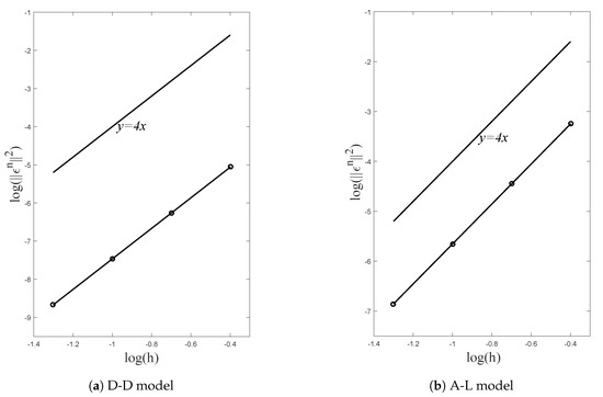
Figure 1. Errors and convergence order at time $t=1.6$.

Table 1. Errors and convergence order of D-D model at time $t=1.6$.

h	$\mathit{\tau }$	${||\mathit{\epsilon }\left(\mathit{T}\right)||}^2\times {10}^6$	Order
0.4	0.00005	8.804684
0.2	0.00005	0.546416	4.01416
0.1	0.00005	0.034090	4.00359
0.05	0.00005	0.002130	4.00086

Table 2. Errors and convergence order of A-L model at time $t=1.6$.

h	$\mathit{\tau }$	${||\mathit{\epsilon }\left(\mathit{T}\right)||}^2\times {10}^4$	Order
0.4	0.00005	5.709740
0.2	0.00005	0.354637	4.01251
0.1	0.00005	0.022128	4.00330
0.05	0.00005	0.001382	4.00083

$\mathbf{Experiment}\mathbf{2}$: In order to determine the convergence order of the Crank–Nicolson method and new difference method, we choose the space step sizes $h=0.4,0.2,0.1,0.05$ and the time step sizes $t=0.008,0.004,0.002,0.001$. Then, we can calculate the truncation error $||{\mathit{\epsilon }}^n{||}_{L_2}^2$, where $||{\mathit{\epsilon }}^n{||}_{L_2}^2=||{\mathbf{w}}^n-{\mathbf{W}}^n{||}_{L_2}^2$. Due to $h:\tau =K$ (K is fixed), we choose to plot “$log(||{\mathit{\epsilon }}^n|{|}_{L_2}^2)$” with respect to “$log\left(h\right)$” in Figure 2. Table 3 and Table 4 and Figure 2 indicate that the convergence order of the Crank–Nicolson method and the new difference method is $O(h^2+{\tau }^2)$ in the $L_2$-norm, which is also in good agreement with the results of Theorems 3 and 4.

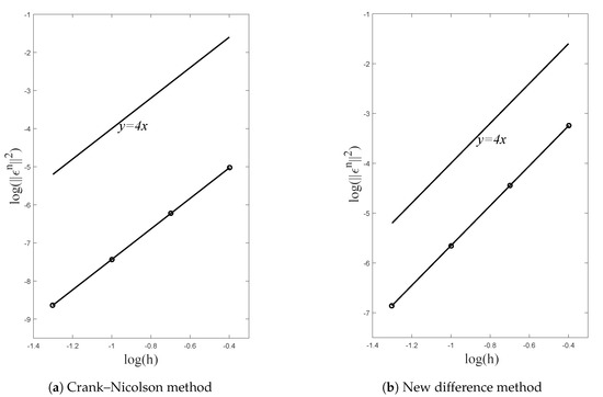
Figure 2. Errors and convergence order at time $t=1.6$.

Table 3. Errors and convergence order of Crank–Nicolson method at time $t=1.6$.

h	$\mathit{\tau }$	$||{\mathit{\epsilon }}^{\mathit{n}}{||}_{{\mathit{L}}_2}^2\times {10}^6$	Order
0.4	0.008	9.490216
0.2	0.004	0.589315	4.01295
0.1	0.002	0.036771	4.00331
0.05	0.001	0.002297	4.00083

Table 4. Errors and convergence order of new difference method at time $t=1.6$.

h	$\mathit{\tau }$	$||{\mathit{\epsilon }}^{\mathit{n}}{||}_{{\mathit{L}}_2}^2\times {10}^4$	Order
0.4	0.008	5.730127
0.2	0.004	0.355952	4.01223
0.1	0.002	0.022211	4.00323
0.05	0.001	0.001388	4.00082

5.2. Numerical Simulation of Dark Solitons’ Motion

$\mathbf{Experiment}\mathbf{3}$: We take the spatial interval $x\in [-125,75]$ and temporal interval from $t=0$ to $t=40$ with two different pairs of integration parameters:

$$h=0.4,\tau =0.02.$$

(34)

The numerical solutions for the Crank–Nicolson method and the new difference method are provided in Figure 3 and Figure 4. From the figures, we can see that the two methods simulate the motion of the one dark soliton for the original NLSE very well. This means that the Crank–Nicolson method and the new difference method have strong convergence, which is consistent with our theories.

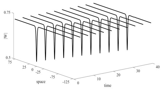
Figure 3. The numerical solutions for the Crank–Nicolson method.

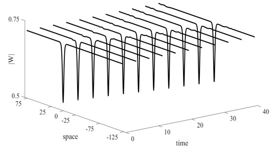
Figure 4. The numerical solutions for the new difference method.

5.3. Preservation of Invariants

In order to further demonstrate the convergence, we check the preservation of the invariants of these models. We introduce the unique property of the original NLSE mentioned in Section 1, which has infinite conserved quantities. If the model can preserve the conserved quantity of the original NLSE very well, it can be confirmed that the numerical solution has high accuracy and is thus convergent. Here, we take the space step size $h=0.4$ and the time step size $\tau =0.02$, $0\le t=n\tau \le 40$ and set $err\left(A\right)\left(t\right)=A\left(t\right)-A\left(0\right)$ for any invariant A.

$\mathbf{Experiment}\mathbf{4}$: For the D-D model, we give the preservation of the invariants $E_1$ and $Q_1$. For the A-L model, the invariants $F_1$ and $F_2$ have both a real part and an imaginary part, so we present the real and imaginary parts of invariants $F_1$ and $F_2$ ($F_m=F{R}_m+iF{I}_m)$, respectively. From Figure 5, both the D-D model and A-L model preserve their invariants well, which means that their numerical solutions have high accuracy. Thus, we can draw the conclusion that the space-symmetric discretization models have a good simulation effect from the trend of the invariants’ error, which further confirms the convergence of these models.

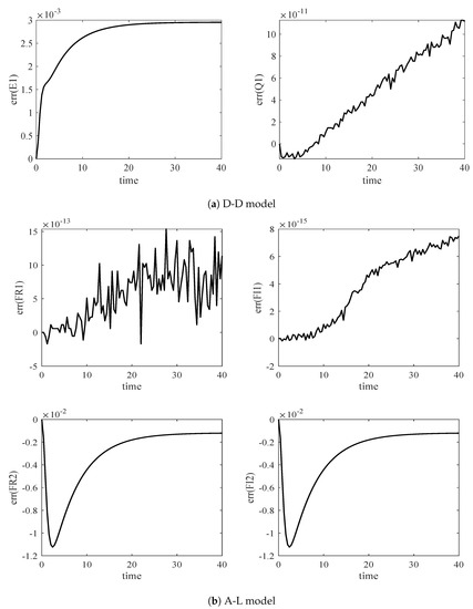
Figure 5. Evolution of invariants by the space-symmetric discretization models.

$\mathbf{Experiment}\mathbf{5}$: We use the conserved quantities’ approximation $S_1$ and $S_2$ ($S_m=S{R}_m+iS{I}_m$) of the original NLSE to test the convergence of the time–space discretization models. As the imaginary part $S{I}_1$ of $S_1$ and the real part $S{R}_2$ of $S_2$ are zero, we only present the evolution of the remaining $S{R}_1$ and $S{I}_2$. Figure 6 shows that the time–space discretization models can maintain the conserved quantities’ approximations $S_1$ and $S_2$ well, which further illustrates the convergence of these models.

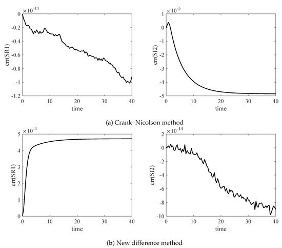
Figure 6. Evolution of invariants by the time–space discretization models.

6. Conclusions

For dark solitons’ motion $(a<0, |W_0(\infty )|=\rho )$, we give two popular space discretization models of the original NLSE by second-order symmetric difference: the direct-discrete model (D-D model) and the Ablowitz–Ladik model (A-L model). On this basis, by applying the midpoint scheme with symmetry to the space-symmetric discretization models, we obtain two time–space discretization models: the Crank–Nicolson method and the new difference method. In dark solitons’ motion, we have proven that the solutions of the D-D model and the A-L model converge to the solution of the original NLSE when $h\to 0$, and their convergence order is $O\left(h^2\right)$ in the defined norm. Through numerical experiments, we give the convergence order to verify the convergence of the space-symmetric discretization models. The results of our numerical experiments are in good agreement with the proven theorems. Furthermore, through theoretical proof, we show that the Crank–Nicolson method and new difference method are of order $O(h^2+{\tau }^2)$ in discrete $L_2$-norm error estimates. The corresponding numerical experiments indicate the convergence of the time–space discretization models, which fit the proven theories well.

In future research, we can simulate D-D model and A-L model via numerical methods with different orders. Comparing the error (for different time step sizes) as a function of the execution time, we can obtain the appropriate figures of the numerical methods. Moreover, we will consider simulation through parallel computing. There is little related work, but it is worth studying.

References

- Ablowitz, M.J.; Segur, H. Solitons and the Inverse Scattering Transform; SIAM: Philadelphia, PA, USA, 1981. [Google Scholar]
- Dodd, R.K.; Eilbeck, J.C.; Gibbon, J.D.; Morris, H.C. Solitons and Nonlinear Wave Equations; Academic Press: New York, NY, USA, 1982. [Google Scholar]
- Hasegawa, A. Optical solitons in fibers. In Optical Solitons in Fibers; Springer: Berlin/Heidelberg, Germany, 1989; pp. 1–74. [Google Scholar]
- Konotop, V.V. Nonlinear Random Waves; World Scientific: Singapore, 1994. [Google Scholar]
- Konotop, V.; Vekslerchik, V. Randomly modulated dark soliton. J. Phys. A Math. Gen. 1991, 24, 767. [Google Scholar] [CrossRef]
- Zakharov, V.E.; Shabat, A.B. Interaction between solitons in a stable medium. Sov. Phys. JETP 1973, 37, 823–828. [Google Scholar]
- Sanz-Serna, J. Methods for the numerical solution of the nonlinear Schrödinger equation. Math. Comput. 1984, 43, 21–27. [Google Scholar] [CrossRef]
- Zhang, L. A high accurate and conservative finite difference scheme for nonlinear Schrödinger equation. Acta Math. Appl. Sin. 2005, 28, 178–186. [Google Scholar]
- Fei, Z.; Pérez-García, V.M.; Vázquez, L. Numerical simulation of nonlinear Schrödinger systems: A new conservative scheme. Appl. Math. Comput. 1995, 71, 165–177. [Google Scholar] [CrossRef]
- Xu, Y.; Shu, C. Local discontinuous Galerkin methods for nonlinear Schrödinger equations. J. Comput. Phys. 2005, 205, 72–97. [Google Scholar] [CrossRef]
- Bratsos, A.; Ehrhardt, M.; Famelis, I.T. A discrete Adomian decomposition method for discrete nonlinear Schrödinger equations. Appl. Math. Comput. 2008, 197, 190–205. [Google Scholar] [CrossRef]
- He, J.H. Homotopy perturbation method: A new nonlinear analytical technique. Appl. Math. Comput. 2003, 135, 73–79. [Google Scholar] [CrossRef]
- Akrivis, G.D. Finite difference discretization of the cubic Schrödinger equation. IMA J. Numer. Anal. 1993, 13, 115–124. [Google Scholar] [CrossRef]
- Borhanifar, A.; Abazari, R. Numerical study of nonlinear Schrödinger and coupled Schrödinger equations by differential transformation method. Opt. Commun. 2010, 283, 2026–2031. [Google Scholar] [CrossRef]
- Zhu, B.; Tang, Y.; Zhang, R.; Zhang, Y. Symplectic simulation of dark solitons motion for nonlinear Schrödinger equation. Numer. Algorithms 2019, 81, 1485–1503. [Google Scholar] [CrossRef]
- Yao, Y.; Xu, M.; Zhu, B.; Feng, Q. Symplectic schemes and symmetric schemes for nonlinear Schrödinger equation in the case of dark solitons motion. Int. J. Model. Simul. Sci. 2021, 12, 2150056. [Google Scholar] [CrossRef]
- Feng, Q.; Huang, J.; Nie, N.; Shang, Z.; Tang, Y. Implementing arbitrarily high-order symplectic methods via Krylov deferred correction technique. Int. J. Model. Simul. Sci. 2010, 1, 277–301. [Google Scholar] [CrossRef]
- Zhu, Y. Implicit difference schemes for the generalized non-linear Schrödinger system. J. Comput. Math. 1983, 1, 116–129. [Google Scholar]
- Guo, B. The convergence of numerical method for nonlinear Schrodinger equation. J. Comput. Math. 1986, 4, 121–130. [Google Scholar]
- Zhang, L.; Chang, Q. A conservative numerical scheme for a class of nonlinear Schrödinger equation with wave operator. Appl. Math. Comput. 2003, 145, 603–612. [Google Scholar] [CrossRef]
- Xie, S.; Li, G.; Yi, S. Compact finite difference schemes with high accuracy for one-dimensional nonlinear Schrödinger equation. Comput. Methods Appl. Mech. Eng. 2009, 198, 1052–1060. [Google Scholar] [CrossRef]
- Wang, T.C.; Guo, B.L. Unconditional convergence of two conservative compact difference schemes for non-linear Schrödinger equation in one dimension. Sci. Sin. Math. 2011, 41, 207–233. [Google Scholar] [CrossRef]
- Li, X.; Zhang, L.; Wang, S. A compact finite difference scheme for the nonlinear Schrödinger equation with wave operator. Appl. Math. Comput. 2012, 219, 3187–3197. [Google Scholar] [CrossRef]
- Li, X.; Zhang, L.; Zhang, T. A new numerical scheme for the nonlinear Schrödinger equation with wave operator. J. Appl. Math. Comput. 2017, 54, 109–125. [Google Scholar] [CrossRef]
- Tang, Y.; Vázquez, L.; Zhang, F.; Pérez-García, V. Symplectic methods for the nonlinear Schrödinger equation. Comput. Math. with Appl. 1996, 32, 73–83. [Google Scholar] [CrossRef]
- Tang, Y.; Pérez-García, V.M.; Vázquez, L. Symplectic methods for the Ablowitz-Ladik model. Appl. Math. Comput. 1997, 82, 17–38. [Google Scholar] [CrossRef]
- Hairer, E.; Lubich, C.; Wanner, G. Geometric Numerical Integration; Springer: Berlin/Heidelberg, Germany, 2002. [Google Scholar]
- Tang, Y.; Cao, J.; Liu, X.; Sun, Y. Symplectic methods for the Ablowitz–Ladik discrete nonlinear Schrödinger equation. J. Phys. Math. Theor. 2007, 40, 24–25. [Google Scholar] [CrossRef]
- Guo, B.; Pascual, P.J.; Rodriguez, M.J.; Vázquez, L. Numerical solution of the sine-Gordon equation. Appl. Math. Comput. 1986, 18, 1–14. [Google Scholar]
Disclaimer/Publisher’s Note: The statements, opinions and data contained in all publications are solely those of the individual author(s) and contributor(s) and not of MDPI and/or the editor(s). MDPI and/or the editor(s) disclaim responsibility for any injury to people or property resulting from any ideas, methods, instructions or products referred to in the content. |
© 2023 by the authors. Licensee MDPI, Basel, Switzerland. This article is an open access article distributed under the terms and conditions of the Creative Commons Attribution (CC BY) license (https://creativecommons.org/licenses/by/4.0/).