Article

On the Approximation of Fractional-Order Differential Equations Using Laplace Transform and Weeks Method

1
Department of Mathematics, Islamia College Peshawar, Peshawar 25120, Khyber Pakhtunkhwa, Pakistan
2
Department of Mathematics and Sciences, Prince Sultan University, P.O. Box 66833, Riyadh 11586, Saudi Arabia
*
Authors to whom correspondence should be addressed.
Symmetry 2023, 15(6), 1214; https://doi.org/10.3390/sym15061214
Submission received: 25 April 2023 / Revised: 31 May 2023 / Accepted: 5 June 2023 / Published: 7 June 2023
(This article belongs to the Special Issue Various Approaches for Generalized Integral Transforms)

Abstract

:
Differential equations of fractional order arising in engineering and other sciences describe nature sufficiently in terms of symmetry properties. In this article, a numerical method based on Laplace transform and numerical inverse Laplace transform for the numerical modeling of differential equations of fractional order is developed. The analytic inversion can be very difficult for complex forms of the transform function. Therefore, numerical methods are used for the inversion of the Laplace transform. In general, the numerical inverse Laplace transform is an ill-posed problem. This difficulty has led to various numerical methods for the inversion of the Laplace transform. In this work, the Weeks method is utilized for the numerical inversion of the Laplace transform. In our proposed numerical method, first, the fractional-order differential equation is converted to an algebraic equation using Laplace transform. Then, the transformed equation is solved in Laplace space using algebraic techniques. Finally, the Weeks method is utilized for the inversion of the Laplace transform. Weeks method is one of the most efficient numerical methods for the computation of the inverse Laplace transform. We have considered five test problems for validation of the proposed numerical method. Based on the comparison between analytical results and the Weeks method results, the reliability and effectiveness of the Weeks method for fractional-order differential equations was confirmed.

1. Introduction

Fractional calculus (FC) is the branch of mathematics investigating the properties of non-integer-order operators. In particular, FC involves the notion and methods of solving differential equations involving fractional derivatives of the unknown. FC is as old as classical calculus. The birth of FC was due to a letter exchange between L’hopital and Libnitz, and its history starts at the end of the 17th century. Many famous mathematicians worked in FC, e.g., Liouville, Riemann, Grunwald, Lagrange, Euler, Heaviside, Fourier, Abel, etc. [1]. One of the fundamental properties of nature is symmetry, and fractional-order differential equations (FDEs) are able to sufficiently describe physical, chemical, or biological processes that have symmetry properties [2]. As a general rule, a physical property may depend on the time moment and the past time, which are actually shown by the utilization of fractional-order operators. In recent years, FDEs have gained importance in both theoretical and applied aspects of several fields, such as biology [3], epidemiology [4], control theory [5], and engineering [6].
The existence and uniqueness of a solution to FDEs given a set of initial conditions is one of the most important results of FDEs. Many researchers have studied the existence and uniqueness results of a solution to FDEs, such as the authors of [7], who studied the existence and uniqueness of FDEs with generalized Caputo’s derivative. Nanware and Dhaigude [8] investigated the existence and uniqueness of FDEs with integral boundary conditions. In [9], the authors studied the existence and uniqueness results of solutions to FDEs with fractional boundary conditions. Other works on the existence and uniqueness of a solution to FDEs can be found in [10] and references therein.
The analytic solution of FDEs has been investigated by the research community using various adequate approaches, such as the Sumudu transform technique [11], the Adomian decomposition method [12], the Akbari–Ganji method [13], the Laplace transform decomposition method [14], the fractional differential transform method [15], the improved subequation method [16], etc. The substantial growth of fractional-order models has led to the emergence of complicated differential equations of fractional order. The analytic solution become hard to obtain for complex problems. Therefore, the desired solution is studied using numerical methods.
Numerous numerical methods have been developed in the literature to approximate the solution of FDEs. The authors of [17] studied the numerical solution of FDEs using the linear extrapolation scheme. Garrappa [18] obtained the numerical solution of FDEs using fractional linear multistep methods. Diethelm et al. [19] utilized the predictor–corrector method for the numerical solution of FDEs. In [20], the authors used the generalized block pulse operational matrix method for obtaining the numerical solution of FDEs. The authors of [21] studied the numerical solution of FDEs using Laplace transform and quadrature. Other works on the numerical solution of FDEs can be found in [22] and references therein.
In this article, our aim is to investigate the numerical solution to FDEs using Laplace transform (LT) and inverse Laplace transform (ILT). Laplace transform has been considered one of the best tools for solving linear differential equations of integer and noninteger orders [23]. Using the LT for solving differential equations, however, sometimes leads to solutions in the Laplace domain that are not readily invertible to the time domain by analytical means. Numerical inversion techniques are used to convert the obtained solution from the Laplace domain into the time domain. Numerous numerical methods are available in the literature for approximating the ILT. Each method has its applications and is suitable for a particular class of problems. Some well-known methods for the numerical approximation of ILT are the Fourier series method [24], the de Hoog method [25], the Stehfest method [26], Talbot’s method [27], etc. The authors of [28] reviewed various algorithms for the approximation of ILT. From experimentation and review, they found that the post-Wilder method [29], the Fourier series method [24], Talbot’s method [27], and the Weeks method [30] are superior methods for approximating the ILT. The Weeks method has the principal advantage over these three methods of returning an analytic formula for the time-domain function. In particular, it assumes that a smooth function can be well approximated by an expansion in terms of Laguerre polynomials [31]. In this method, the unknown coefficients are evaluated once for all for any given transformed function. Furthermore, it is equally applicable to real and complex time-domain functions [32].
In this paper, we aim to use the Weeks method to approximate the solution of FDEs.
The paper is organized as follows. In Section 2, we briefly introduce some basic concepts from fractional calculus. The proposed methods is discussed in Section 3. In Section 4, numerical examples are provided. Finally, Section 5 provides conclusions related to these studies.

2. Preliminaries

Definition 1. 
Let the function C ( t ) be piecewise continuous for t > 0 and of exponential order; then, the Laplace transform (LT) of C ( t ) is defined as [33]
L { C ( t ) } = C ^ ( s ) = 0 e x p ( s t ) C ( t ) d t
where s is the complex variable known as the Laplace variable.
Definition 2 
([33]). A function C ( t ) is said to be of exponential order ρ 0 > 0 on 0 t < if for M > 0 and t > 0
| C ( t ) | M e ( ρ 0 t ) ,
or, equivalently,
lim t e x p ( η t ) | C ( t ) | = 0 , η > ρ 0 .
Definition 3. 
The Mittag-Leffler (ML) function plays a key role in the solution of differential equations of fractional order.
1. 
The ML function in one parameter is defined as [34]
E η ( ζ ) = k = 0 ζ k Γ ( η k + 1 ) ,
where ζ C , and η is an arbitrary positive constant. The LT of the ML function in one parameter is given as
L { E η ( β ζ η ) } = s η 1 s η + β ,
where R e ( s ) > | β | 1 / η .
2. 
The ML function in two parameters is defined as [34]
E η , σ ( ζ ) = k = 0 ζ k Γ ( η k + σ ) ,
where ζ C , and η and σ are arbitrary positive constants. The LT of the ML function in two parameter is given as
L { ζ σ 1 E η , σ ( β ζ η ) } = s η σ s η + β ,
where R e ( s ) > | β | 1 / η .
3. 
The ML function in three parameters is defined as [34]
E η , σ δ ( ζ ) = k = 0 ( δ ) k ζ k Γ ( η i + σ ) k !
where ζ C , η,  σ, and δ are arbitrary positive constants, and ( δ ) k is a Pochhammer symbol [23]. The LT of the ML function in three parameters is given as
L { ζ σ 1 E η , σ δ ( β ζ η ) } = s η δ σ ( s η + β ) δ ,
where R e ( s ) > | β | 1 / η .
Definition 4. 
The Caputo derivative is defined as [34]
0 c D t α C ( t ) = 1 Γ ( p α ) 0 t d p C ( s ) d s p ( t s ) p α + 1 d s ,   p 1 < α p .
The LT of the Caputo derivative is given by [34]
L 0 c D t α C ( t ) = s α C ^ ( s ) k = 0 p 1 s α k 1 C ( k ) ( 0 ) .
Definition 5. 
Let C ( t ) possess a continuous derivative and be of exponential order ρ 0 . Then, the inversion of C ^ ( s ) is given by the integral [34]
C ( t ) = 1 2 π i ρ i ρ + i C ^ ( s ) e s t d s ,   w h e r e   ρ > ρ 0 ,
Definition 6. 
The Weeks method is one of the most well-known algorithms for the numerical inversion of a Laplace space function. It returns an explicit expression for the time-domain function as an expansion in Laguerre polynomials, given as
C ( t ) = e σ t m = 0 a m e β t L m ( 2 β t ) , t > 0 ,
where the a m are the expansion coefficients defined by
2 β 1 μ C ^ ρ + 2 β 1 μ β = m = 0 a m μ m ,   | μ | < R ,
where L m ( t ) denotes the Laguerre polynomial of degree m , and β is a positive real number.

3. Proposed Method

Here, we discuss our proposed numerical method for the numerical solution of FDEs. Our numerical method comprises three main steps: (i) we consider an FDE and reduce it to an algebraic using the Laplace transform; (ii) the solution of the reduced equation is obtained using algebraic techniques in the LT domain; and (iii) the solution of the original problem is obtained using the ILT. However, the analytic inversion is hard to compute. Therefore, we use the Weeks method for the numerical inversion of the LT. Figure 1 shows the flowchart of the proposed numerical scheme.

3.1. Time-Fractional Differential Equation

We consider a time-fractional initial value problem given as
0 c D t α C ( t ) + D t 2 C ( t ) + D t C ( t ) + C ( t ) = f ( t ) ,   p 1 < α p ,
with initial condition
C ( k ) ( 0 ) = C 0 ( k ) ,   k = 0 , 1 , 2 , ,   p 1 .
Applying Laplace transform to Equation (9), we obtain
L 0 c D t α C ( t ) + D t 2 C ( t ) + D t C ( t ) + C ( t ) = L f ( t ) ,
s α C ^ ( s ) k = 0 p 1 s α k 1 C ( k ) ( 0 ) + s 2 C ^ ( s ) s C ( 0 ) C ( 1 ) ( 0 ) + s C ^ ( s ) C ( 0 ) + C ^ ( s ) = f ^ ( s ) ,
( s α + s 2 + s + 1 ) C ^ ( s ) = k = 0 p 1 s α k 1 C ( k ) ( 0 ) + s C ( 0 ) + C ( 1 ) ( 0 ) + C ( 0 ) + f ^ ( s ) ,
C ^ ( s ) = ( s α + s 2 + s + 1 ) 1 k = 0 p 1 s α k 1 C ( k ) ( 0 ) + s C ( 0 ) + C ( 1 ) ( 0 ) + C ( 0 ) + f ^ ( s ) ,
applying the ILT, we obtain
C ( t ) = 1 2 π i ρ i ρ + i e s t C ^ ( s ) d s = 1 2 π i Γ e s t C ^ ( s ) d s , ρ > ρ 0 .
Here, C ^ ( s ) is the transformed function that needs to be inverted, ρ 0 is the convergence abscissa, and ρ > ρ 0 means that all the singularities of C ^ ( s ) lie in the open half-plane R e s < ρ . The analytic evaluation of the integral in Equation (11) can be challenging for the complex forms of transformed function C ^ ( s ) . Therefore, numerical methods are used to evaluate the integral in Equation (11). The ILT is generally an ill-posed problem. The numerical inversion of LT is a long-standing issue that has led to various numerical inverse Laplace transform (NILT) approaches [22]. In this work, we use the Weeks method for the computation of the integral in Equation (11).

3.2. Weeks Method

In the Weeks method, the Bromwich line is parameterized as s = ρ + i y ,   y R to obtain the Fourier integral
C ( t ) = e ρ t 2 π e i t y C ^ ( ρ + i y ) d y .
The transform C ^ ( ρ + i y ) is then expanded as
C ^ ( ρ + i y ) = m = a m ( i y β ) m ( i y + β ) m + 1 ,   β > 0 ,   y R .
Using Equation (13) in Equation (12), we obtain
C ( t ) = e ρ t 2 π m = a m ψ m ( t ; β ) ,
where
ψ m ( t ; β ) = e i t y ( i y β ) m ( i y + β ) m + 1 d y .
The Fourier integral may be evaluated using residues, and for t > 0 , one obtains
ψ m ( t ; β ) = 2 π e β t L m ( 2 β t ) , m 0 , 0 , m < 0 .
where L m ( t ) denotes the mth degree Laguerre polynomial, and where ρ > ρ 0 , β R + are the parameters, and ρ 0 is the convergence abscissa. The Laguerre polynomials are defined by
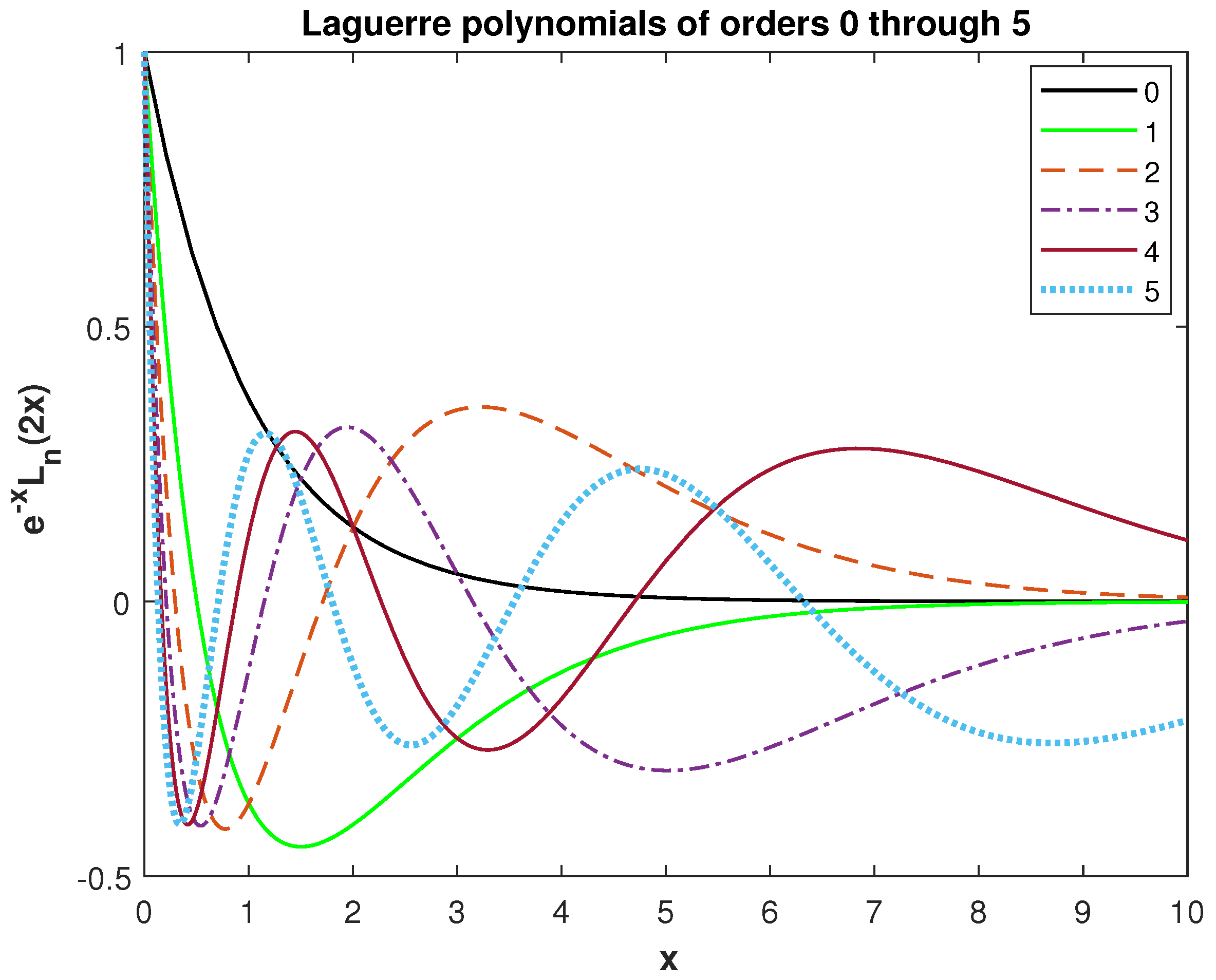
L m ( x ) = e x m ! d m d x m ( e x x m ) ,
and see the Figure 2.
Where a m are Taylor coefficients of
Q ( μ ) = 2 β 1 μ C ^ ρ + 2 β 1 μ β = m = 0 a m μ m ,   | μ | < R ,
where R is the radius of convergence of the Maclaurin series (18). The coefficients a m are computed using Cauchy’s formula as
a m = 1 2 π i | μ | = 1 Q ( μ ) μ m + 1 d μ = 1 2 π π π Q ( e i ϑ ) e i m ϑ d ϑ ,
the integral in Equation (19) can be approximated using the midpoint rule as
a ˜ m = e i m h / 2 2 N j = N N 1 Q ( e i ϑ j + 1 / 2 ) e i m ϑ j ,   m = 0 ,   1 ,   2 ,   3 ,   ,   N 1 ,
where ϑ j = j h , h = π N . This can be evaluated as an FFT of length 2 N or as N separate summations.

Error Analysis

In this section, we analyze the error of the proposed method. The author of  [35] observed that for the expansion given below
C ( t ) = e x p ( ρ t ) m = 0 a m e x p ( β t ) L m ( 2 β t ) .
There are three reason due to which the error arises:
  • First is the truncation of the series to N terms;
  • Second is the computation of the expansion coefficients numerically;
  • Third is the approximation of ILT numerically. This error in (21) reveals itself in the fact that any error in the evaluated coefficients are increased with increasing t when ρ > 0 .
The actual expansion for modeling these three errors is
C ˜ ( t ) = e x p ( ρ t ) m = 0 N 1 a ˜ m ( 1 + ϵ m ) e x p ( β t ) L m ( 2 β t ) ,
and ϵ m is the relative error in the floating-point representation of the coefficients, i.e., f l ( a ˜ m ) = a ˜ m ( 1 + ϵ m ) .
Subtraction of Equation (22) from Equation (21) with assumption m = 0 | a m | < yields
| C ( t ) C ˜ ( t ) | e x p ( ρ t ) ( T r n + D i s + C o n ) ,
where T r n = m = N | a m | , D i s = m = 0 N 1 | a m a ˜ m | , and C o n = ϵ m = 0 N 1 | a ˜ m | are the truncation, discretization, and conditioning error bounds, respectively, and ϵ is the machine roundoff unit satisfying max 0 m N 1 | ϵ m | ϵ with the fact that | e x p ( β t ) L m ( 2 β t ) | 1 . The D i s error can be neglected when compared with the T r n and C o n errors [35]. Therefore, we refer to the T r n error and C o n error. The upper bounds for the T r n error and C o n error were give in  [35] as
T r n m ( δ ) δ N ( δ 1 ) ,   C o n ϵ δ m ( δ ) δ 1 ,
valid for δ ( 1 , R ) . Therefore, the following error bound is obtained
E e s t m ( δ ) δ N ( δ 1 ) + ϵ δ m ( δ ) δ 1 .
For optimal E e s t , the author of [35] proposed two algorithms for the computation of the parameters ρ and β . In this work, we utilized the following Algorithm 1, proposed in [35].   
Algorithm 1 Computation of ( ρ , β )
The user needs to provide F ( s ) , t, and N, and a rectangle [ ρ 0 , ρ m a x ] × [ 0 , β m a x ] , which likely contains the optimal values of ρ and β . The algorithm then works by solving
ρ = { ρ [ ρ 0 , ρ m a x ] | E e s t ( ρ , β ( ρ ) ) = m i n i m u m } ,
where
β ( ρ ) = { β [ 0 , β m a x ] | T r n ( ρ , β ) = m i n i m u m } .

4. Numerical Results and Discussions

In many situations, analytic techniques are unavailable for obtaining the solution of differential equations of fractional order. So, we need to utilize numerical techniques for FDEs. This section aims to demonstrate the efficiency and simplicity of the proposed method for differential equations of fractional order. Five numerical examples are selected to validate the proposed method. The results show that the proposed method is accurate and easy to implement. We performed our experiments in MATLAB R2018a on a Windows 10 (64-bit) PC equipped with an Intel(R) Core(TM) i5-3317U CPU @ 1.70 GHz and with 4 GB of RAM. The numerical error is measured using two error norms, the absolute error and the relative error, defined by
A E = | C a p ( t ) C ( t ) | ,
and
R E = C a p ( t ) C ( t ) C a p ( t ) ,
where C a p ( t ) and C ( t ) are the approximate and exact solutions, respectively. In all the numerical examples, the initial conditions and the linear source term f ( t ) are selected according to the exact solution.

4.1. Example 1

We consider a fractional initial value problem of the form [21]
d C ( t ) d t + d α C ( t ) d t α = f ( t ) ,
the exact solution of the problem is given as
C ( t ) = E 1 + α ( t 1 + α ) + 0 t E 1 + α ( τ 1 + α ) f ( t τ ) d τ ,
the substitution τ = t y 2 yields
C ( t ) = E 1 + α ( t 1 + α ) + 0 t E 1 + α ( t 1 + α y 2 + 2 α ) f ( t t y 2 ) 2 t y d y .
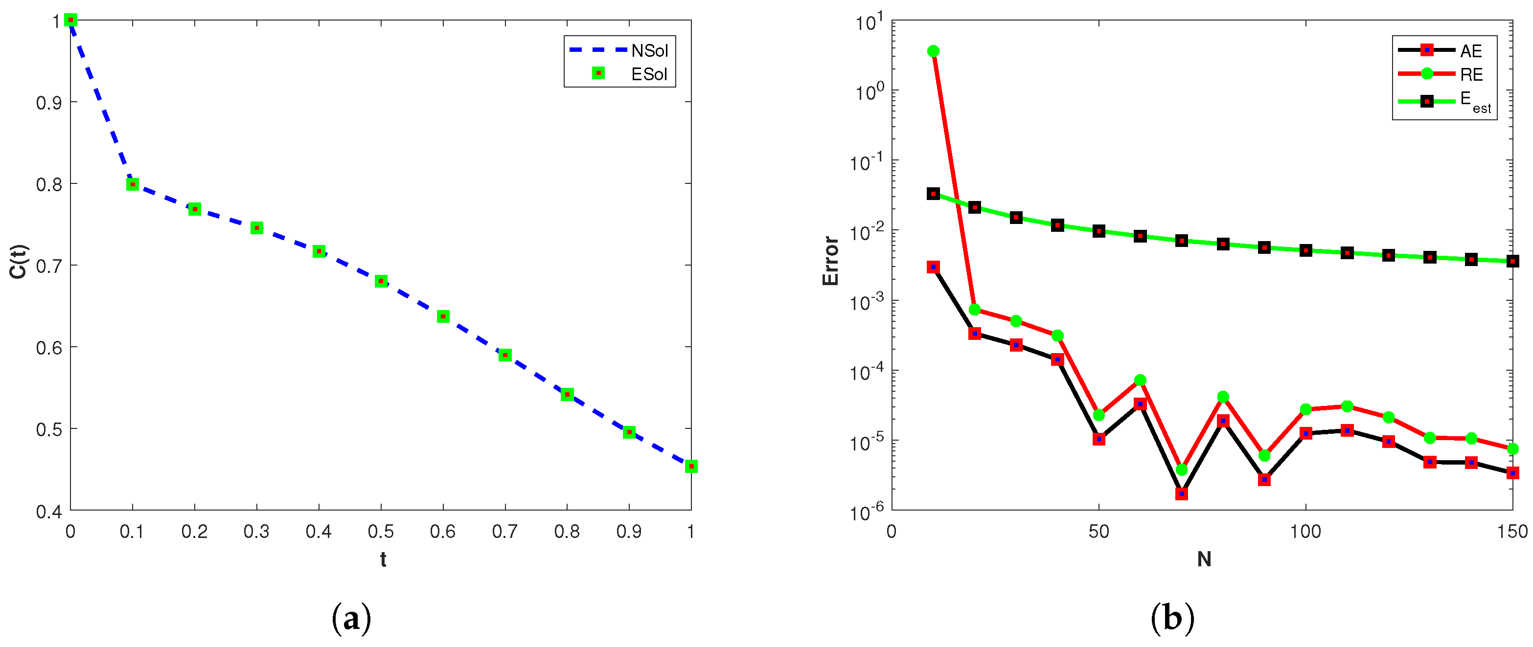
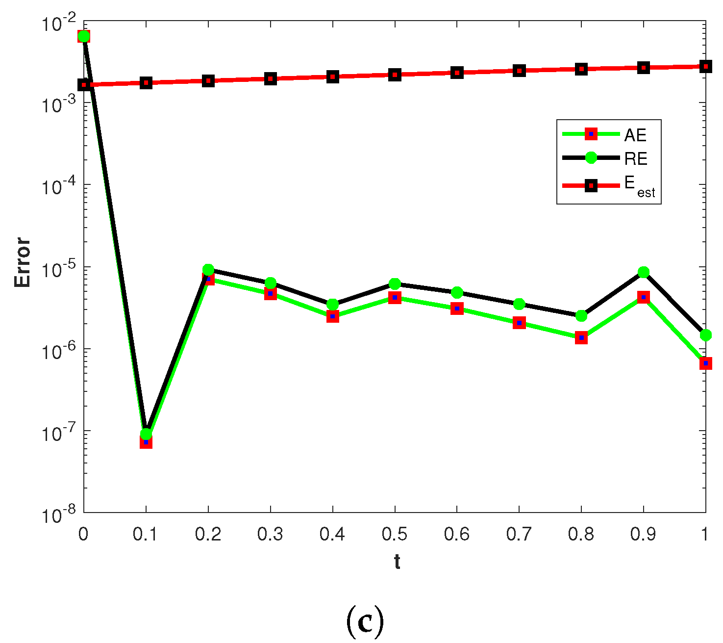
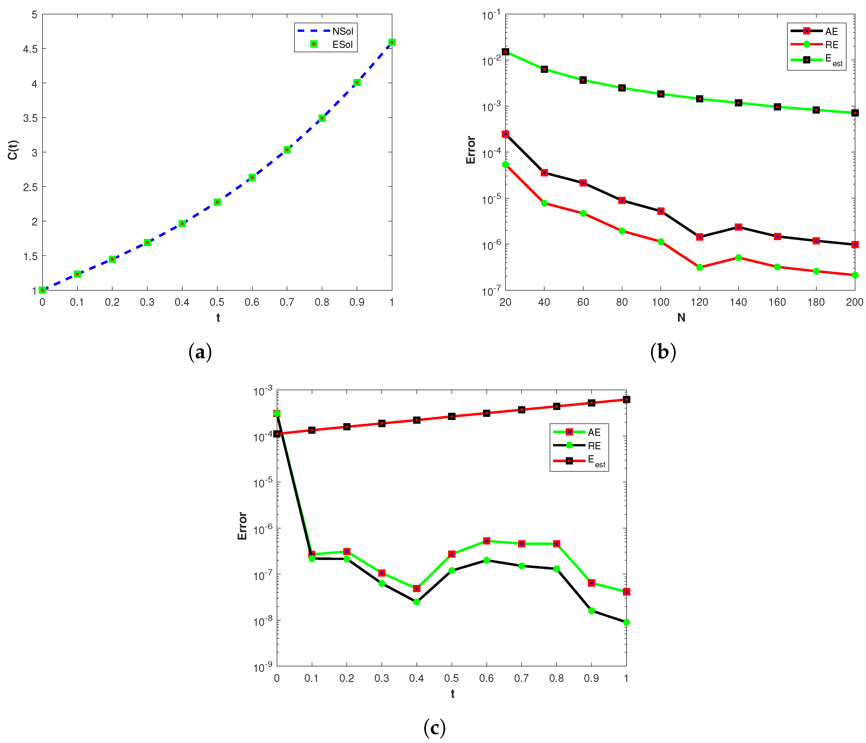
This problem is solved using the proposed method with α = 1 2 . The absolute error ( A E ) , the relative error ( R E ) , and the error estimates ( E e s t ) for various values of N with optimal values of the parameters ( ρ , β ) are shown in Table 1. The plot of the exact solution ( E s o l ) and numerical solution ( N s o l ) is shown in Figure 3a. The comparison of A E , R E , and ( E e s t ) versus N at t = 1 is shown in Figure 3b. Similarly, the comparison of A E , R E , and ( E e s t ) versus t with N = 200 is presented in Figure 3c. From the obtained results, we can see that the method has high accuracy and the computational results are in good agreement with the theoretical results.

4.2. Example 2

We consider a fractional initial value problem of the form [36]
d α C ( t ) d t α + C ( t ) = f ( t ) ,
the exact solution of the problem is given as
C ( t ) = E α ( t α ) .
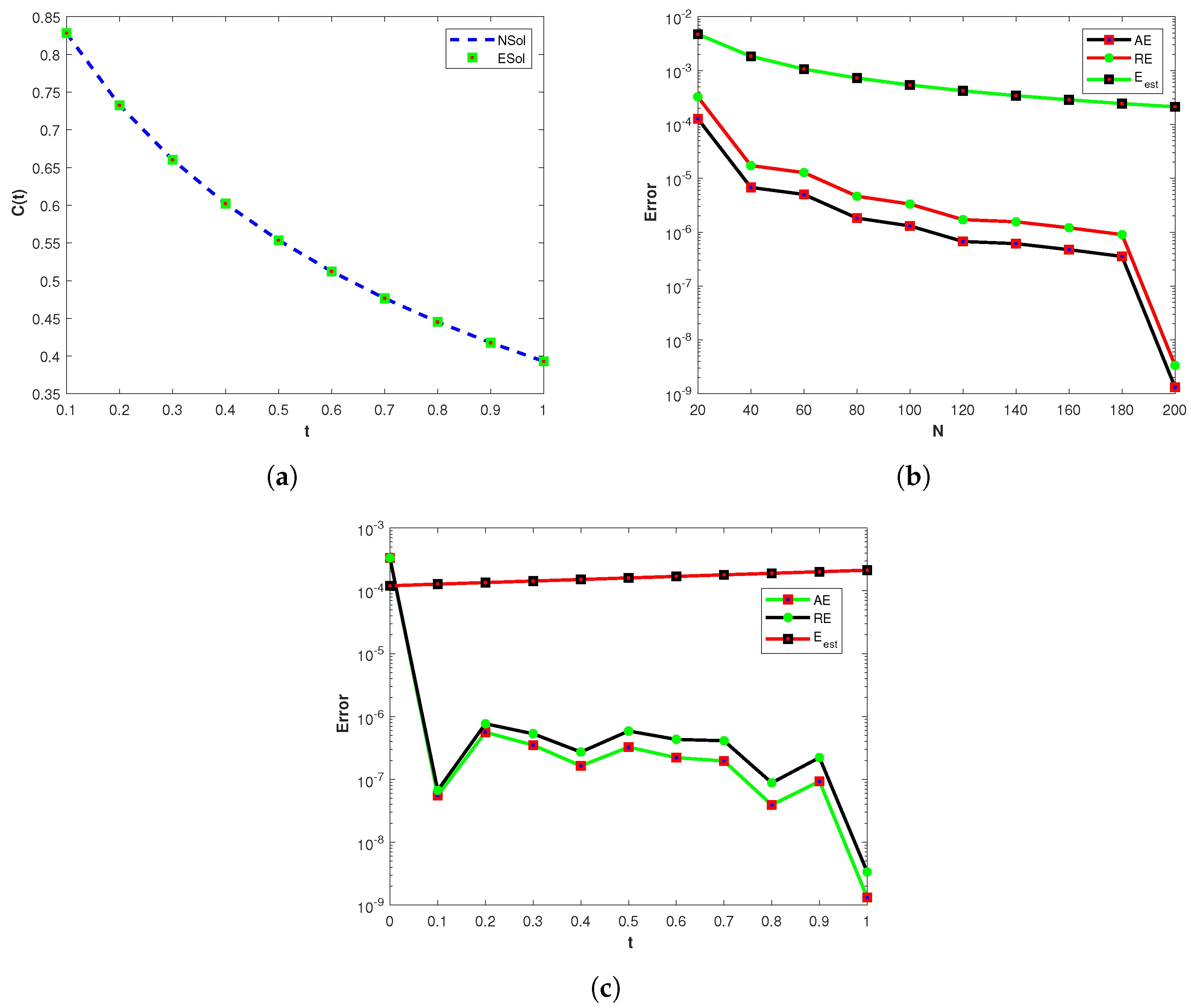
We applied the proposed method to solve the problem with optimal values of the parameters ( ρ , β ) , α = 3 4 , and various values of N . The numerical solutions obtained by the present method and another numerical method [36] are given in Table 2. Clearly, the numerical results show that the present method is effective, and its accuracy is comparable with existing methods. The plot of the exact solution ( E s o l ) and numerical solution ( N s o l ) is shown in Figure 4a. The comparison of A E , R E , and E e s t versus N at t = 1 is shown in Figure 4b. Similarly, the comparison of A E , R E , and E e s t versus t with N = 200 is presented in Figure 4c. It is observed that the computational results using the proposed method are in good agreement with the exact solutions.

4.3. Example 3

We consider a linear fractional initial value problem of the form [37]
d α C ( t ) d t α = f ( t ) + C ( t ) ,
the exact solution of the problem is given as
C ( t ) = E α ( t α ) + 1 Γ ( 1 α ) 0 t ( t τ ) α E α ( t α ) t α Γ ( α + 1 ) 1 d τ ,
or C ( t ) can be written as
C ( t ) = k = 0 t k α Γ ( k α + 1 ) + t j = 1 t j α Γ ( j α + 2 ) .
This problem is solved using the proposed method with α = 3 4 . The absolute error A E , the relative error R E , and the error estimates ( E e s t ) for various values of N with optimal values of the parameters ( ρ , β ) are shown in Table 3. The plot of the exact solution ( E s o l ) and numerical solution ( N s o l ) is shown in Figure 5a. The comparison of A E , R E , and E e s t versus N at t = 1 is shown in Figure 5b. Similarly, the comparison of A E , R E , and E e s t versus t with N = 220 is presented in Figure 5c. It is observed that the numerical solution obtained using the proposed method is in excellent agreement with the analytic solution of the method proposed in [37].

4.4. Example 4

We consider a linear fractional initial value problem of the form [38]
d C ( t ) d t + d α C ( t ) d t α + C ( t ) = f ( t ) ,
the exact solution of the problem is given as
C ( t ) = t 2 t ,
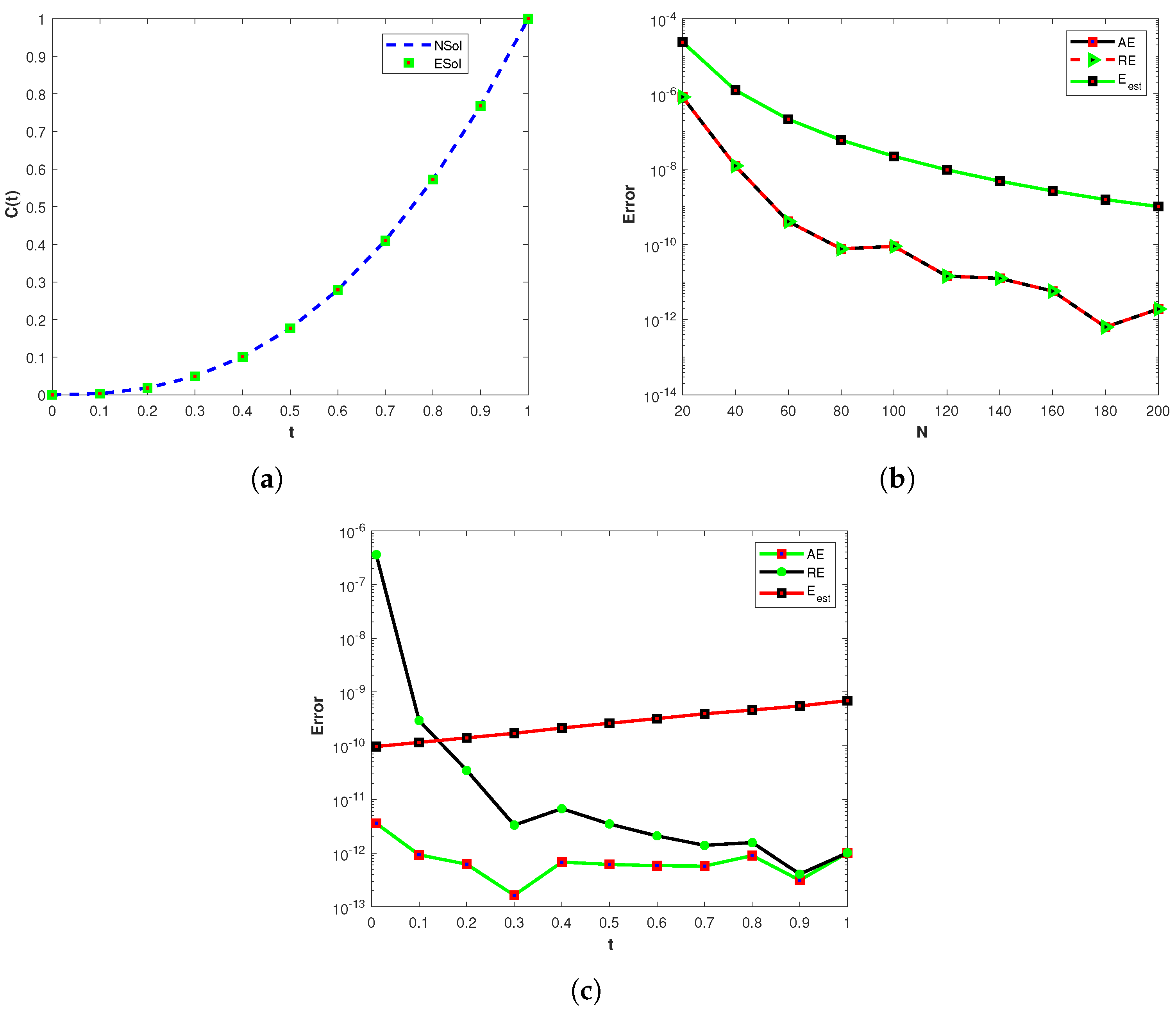
This problem is solved using the proposed method with α = 1 4 . The initial condition is selected according to the exact solution. The absolute error A E , the relative error R E , and the error estimates ( E e s t ) for various values of N with optimal values of the parameters ( ρ , β ) are shown in Table 4. The plot of the exact solution ( E s o l ) and numerical solution ( N s o l ) is shown in Figure 6a. The comparison of A E , R E , and E e s t versus N at t = 1 is shown in Figure 6b. Similarly, the comparison of A E , R E , and E e s t versus t with N = 220 is presented in Figure 6c. It is observed that the proposed method performed better than another Laplace transform method proposed in [38].

4.5. Example 5

We consider a linear fractional initial value problem of the form [39]
d α C ( t ) d t α + C ( t ) = f ( t ) ,
the exact solution of the problem is given as
C ( t ) = t α E α , α + 1 ( t α ) .
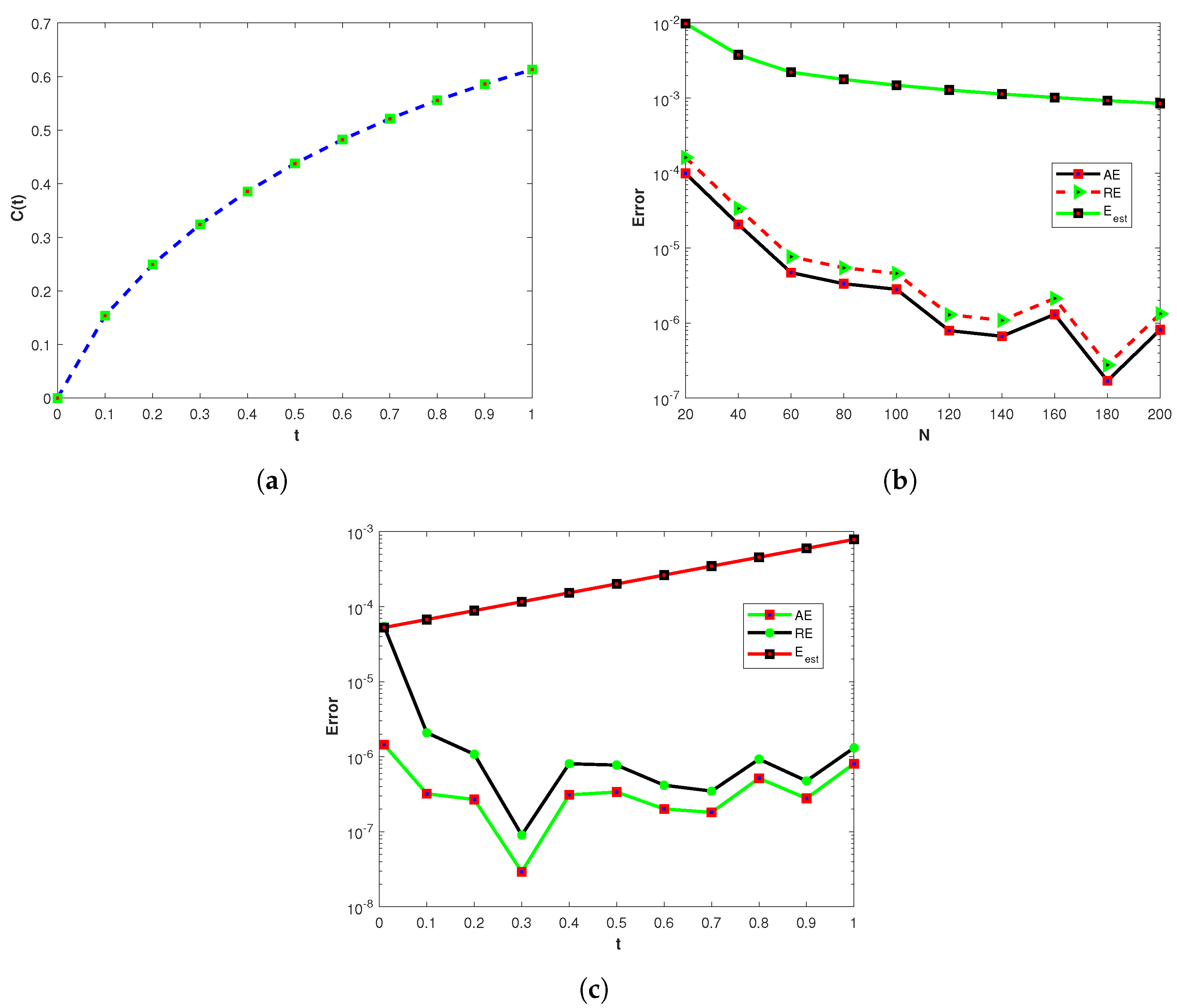
This problem is solved using the proposed method with α = 0.8 . The initial condition is selected according to the exact solution. The absolute error A E , the relative error R E , and the error estimates ( E e s t ) for various values of N with optimal values of the parameters ( ρ , β ) are shown in Table 5. The plot of the exact solution ( E s o l ) and numerical solution ( N s o l ) is shown in Figure 7a. The comparison of A E , R E , and E e s t versus N at t = 1 is shown in Figure 7b. Similarly, the comparison of A E , R E , and E e s t versus t with N = 220 is presented in Figure 7c. We see that the computational results of the proposed method are in good agreement with the results presented in [39].

5. Conclusions

In this article, an efficient method based on Laplace transform and inverse Laplace transform was proposed for the numerical modeling of FDEs in Caputo’s sense. The Laplace transform provides a powerful tool for analyzing linear FDEs. However, many physical problems lead to Laplace transforms whose inverses cannot be obtained by analytic techniques. Several numerical methods are described in the literature to address the issues related to the inverse Laplace transform. In this work, we used the Weeks method, which is one of the most popular methods for the numerical inversion of the Laplace transform. We evaluated the method for five different test problems. The computational results are presented in the form of tables and figures. The obtained results led us to the conclusion that the Weeks method provides an accurate and stable approach to the numerical approximation of the solution of fractional differential equations. The application of the Weeks method coupled with some spatial discretization techniques for the numerical modeling of time-fractional PDEs may be of future interest.

Author Contributions

Conceptualization, K. and S.U.K.; methodology, K.; software, K. and S.U.K.; validation, S.U.K., S.H. and N.M.; formal analysis, N.M.; investigation, S.H.; resources, S.H.; data curation, N.M.; writing—original draft preparation, K.; writing—review and editing, K. and S.H.; visualization, N.M.; supervision, K.; project administration, N.M.; funding acquisition, S.H. All authors have read and agreed to the published version of the manuscript.

Funding

This research is supported by Prince Sultan University.

Data Availability Statement

All data required for this research are included within the paper.

Acknowledgments

The authors S. Haque and N. Mlaiki would like to thank the Prince Sultan University for paying the publication fees for this work through TAS LAB.

Conflicts of Interest

The authors declare no conflict of interest.

References

  1. Oldham, K.; Spanier, J. The Fractional Calculus Theory and Applications of Differentiation and Integration to Arbitrary Order; Elsevier: Amsterdam, The Netherlands, 1974. [Google Scholar]
  2. Kamran; Shah, F.A.; Aly, W.H.F.; Aksoy, H.; Alotaibi, F.M.; Mahariq, I. Numerical Inverse Laplace Transform Methods for Advection-Diffusion Problems. Symmetry 2022, 14, 2544. [Google Scholar] [CrossRef]
  3. Hattaf, K.; Yousfi, N. Global stability for fractional diffusion equations in biological systems. Complexity 2020, 2020, 5476842. [Google Scholar] [CrossRef]
  4. Shah, K.; Abdeljawad, T. Study of a mathematical model of COVID-19 outbreak using some advanced analysis. Waves Random Complex Media 2022, 33, 1–18. [Google Scholar] [CrossRef]
  5. Ali, A.; Khalid, S.; Rahmat, G.; Kamran; Ali, G.; Nisar, K.S.; Alshahrani, B. Controllability and Ulam–Hyers stability of fractional order linear systems with variable coefficients. Alex. Eng. J. 2022, 61, 6071–6076. [Google Scholar] [CrossRef]
  6. Kamran; Asif, M.; Shah, K.; Abdalla, B.; Abdeljawad, T. Numerical solution of Bagley–Torvik equation including Atangana-Baleanu derivative arising in fluid mechanics. Results Phys. 2023, 49, 106468. [Google Scholar] [CrossRef]
  7. Gambo, Y.Y.; Ameen, R.; Jarad, F.; Abdeljawad, T. Existence and uniqueness of solutions to fractional differential equations in the frame of generalized Caputo fractional derivatives. Adv. Differ. Equ. 2018, 2018, 134. [Google Scholar] [CrossRef] [Green Version]
  8. Nanware, J.A.; Dhaigude, D.B. Existence and uniqueness of solutions of differential equations of fractional order with integral boundary conditions. J. Nonlinear Sci. Appl. 2014, 7, 246–254. [Google Scholar] [CrossRef] [Green Version]
  9. Saha, K.K.; Sukavanam, N.; Pan, S. Existence and uniqueness of solutions to fractional differential equations with fractional boundary conditions. Alex. Eng. J. 2023, 72, 147–155. [Google Scholar] [CrossRef]
  10. Boulares, H.; Ardjouni, A.; Laskri, Y. Existence and uniqueness of solutions to fractional order nonlinear neutral differential equations. Appl. Math. E–Notes 2018, 18, 25–33. [Google Scholar]
  11. Gill, V.; Modi, K.; Singh, Y. Analytic solutions of fractional differential equation associated with RLC electrical circuit. J. Stat. Manag. Syst. 2018, 21, 575–582. [Google Scholar] [CrossRef]
  12. Shi, X.C.; Huang, L.L.; Deng, Z.G.; Liu, D. Analytical solutions of fractional differential equations using the convenient adomian series. Abstr. Appl. Anal. 2014, 2014, 284967. [Google Scholar] [CrossRef] [Green Version]
  13. Attar, M.A.; Roshani, M.; Hosseinzadeh, K.; Ganji, D.D. Analytical solution of fractional differential equations by Akbari–Ganji’s method. Partial. Differ. Equ. Appl. Math. 2022, 6, 100450. [Google Scholar] [CrossRef]
  14. Jia, H. Analytical Solutions for Fractional Differential Equations Using a General Conformable Multiple Laplace Transform Decomposition Method. Symmetry 2023, 15, 389. [Google Scholar] [CrossRef]
  15. Ibis, B.; Bayram, M.; Agargun, A.G. Applications of fractional differential transform method to fractional differential-algebraic equations. Eur. J. Pure Appl. Math. 2011, 4, 129–141. [Google Scholar]
  16. Karaagac, B. New exact solutions for some fractional order differential equations via improved sub-equation method. Discrete Contin. Dyn. Syst. 2019, 12, 447–454. [Google Scholar] [CrossRef] [Green Version]
  17. Ford, N.J.; Simpson, A.C. The numerical solution of fractional differential equations: Speed versus accuracy. Numer. Algorithms 2001, 26, 333–346. [Google Scholar] [CrossRef]
  18. Garrappa, R. Numerical solution of fractional differential equations: A survey and a software tutorial. Mathematics 2018, 6, 16. [Google Scholar] [CrossRef] [Green Version]
  19. Diethelm, K.; Ford, N.J.; Freed, A.D. A predictor-corrector approach for the numerical solution of fractional differential equations. Nonlinear Dyn. 2002, 29, 3–22. [Google Scholar] [CrossRef]
  20. Li, Y.; Sun, N. Numerical solution of fractional differential equations using the generalized block pulse operational matrix. Comput. Math. Appl. 2011, 62, 1046–1054. [Google Scholar] [CrossRef] [Green Version]
  21. Uddin, M.; Khan, S.; Kamran. On the numerical solution of fractional order differential equations using transforms and quadrature. TWMS J. Appl. Eng. Math. 2019, 8, 267–274. [Google Scholar]
  22. Kamran; Ahmad, S.; Shah, K.; Abdeljawad, T.; Abdalla, B. On the Approximation of Fractal-Fractional Differential Equations Using Numerical Inverse Laplace Transform Methods. Comput. Model. Eng. Sci. 2023, 135, 2743–2765. [Google Scholar] [CrossRef]
  23. Sheng, H.; Li, Y.; Chen, Y. Application of numerical inverse Laplace transform algorithms in fractional calculus. J. Frankl. Inst. 2011, 348, 315–330. [Google Scholar] [CrossRef]
  24. Crump, K.S. Numerical inversion of Laplace transforms using a Fourier series approximation. J. ACM 1976, 23, 89–96. [Google Scholar] [CrossRef]
  25. De Hoog, F.R.; Knight, J.H.; Stokes, A.N. An improved method for numerical inversion of Laplace transforms. SIAM J. Sci. Stat. Comput. 1982, 3, 357–366. [Google Scholar] [CrossRef]
  26. Stehfest, H. Algorithm 368: Numerical inversion of Laplace transforms [D5]. Commun. ACM 1970, 13, 47–49. [Google Scholar] [CrossRef]
  27. Talbot, A. Theaccurate numerical inversion of Laplace transforms. IMA J. Appl. Math. 1979, 23, 97–120. [Google Scholar] [CrossRef] [Green Version]
  28. Davies, B.; Martin, B. Numerical inversion of the Laplace transform: A survey and comparison of methods. J. Comput. Phys. 1979, 33, 1–32. [Google Scholar] [CrossRef]
  29. Abate, J.; Valkó, P.P. Multi-precision Laplace transform inversion. Int. J. Numer. Methods Eng. 2004, 60, 979–993. [Google Scholar] [CrossRef]
  30. Weeks, W.T. Numerical inversion of Laplace transforms using Laguerre functions. J. ACM (JACM) 1966, 13, 419–429. [Google Scholar] [CrossRef]
  31. Abate, J.; Choudhury, G.L.; Whitt, W. On the Laguerre method for numerically inverting Laplace transforms. INFORMS J. Comput. 1996, 8, 413–427. [Google Scholar] [CrossRef] [Green Version]
  32. Brio, M.; Kano, P.O.; Moloney, J.V. Application of Weeks method for the numerical inversion of the Laplace transform to the matrix exponential. Commun. Math. Sci. 2005, 3, 335–372. [Google Scholar] [CrossRef] [Green Version]
  33. Kilbas, A.A.; Srivastava, H.M.; Trujillo, J.J. Theory and applications of fractional differential equations. In North-Holland Mathematics Studies; Elsevier: Amsterdam, The Netherlands, 2006; Volume 204. [Google Scholar]
  34. Kilbas, A.A.; Saigo, M.; Saxena, R.K. Generalized Mittag-Leffler function and generalized fractional calculus operators. Integral Transform. Spec. Funct. 2004, 15, 31–49. [Google Scholar] [CrossRef]
  35. Weideman, J.A.C. Algorithms for parameter selection in the Weeks method for inverting the Laplace transform. SIAM J. Sci. Comput. 1999, 21, 111–128. [Google Scholar] [CrossRef]
  36. Kumar, P.; Agrawal, O.P. An approximate method for numerical solution of fractional differential equations. Signal Process. 2006, 86, 2602–2610. [Google Scholar] [CrossRef]
  37. Weilbeer, M. Efficient Numerical Methods for Fractional Differential Equations and Their Analytical Background. Ph.D. Thesis, Technische Universität Braunschweig, Braunschweig, Germany, 2005. [Google Scholar]
  38. Rani, D.; Mishra, V.; Cattani, C. Numerical inverse Laplace transform for solving a class of fractional differential equations. Symmetry 2019, 11, 530. [Google Scholar] [CrossRef] [Green Version]
  39. Podlubny, I. Matrix approach to discrete fractional calculus. Fract. Calc. Appl. Anal. 2000, 3, 359–386. [Google Scholar]
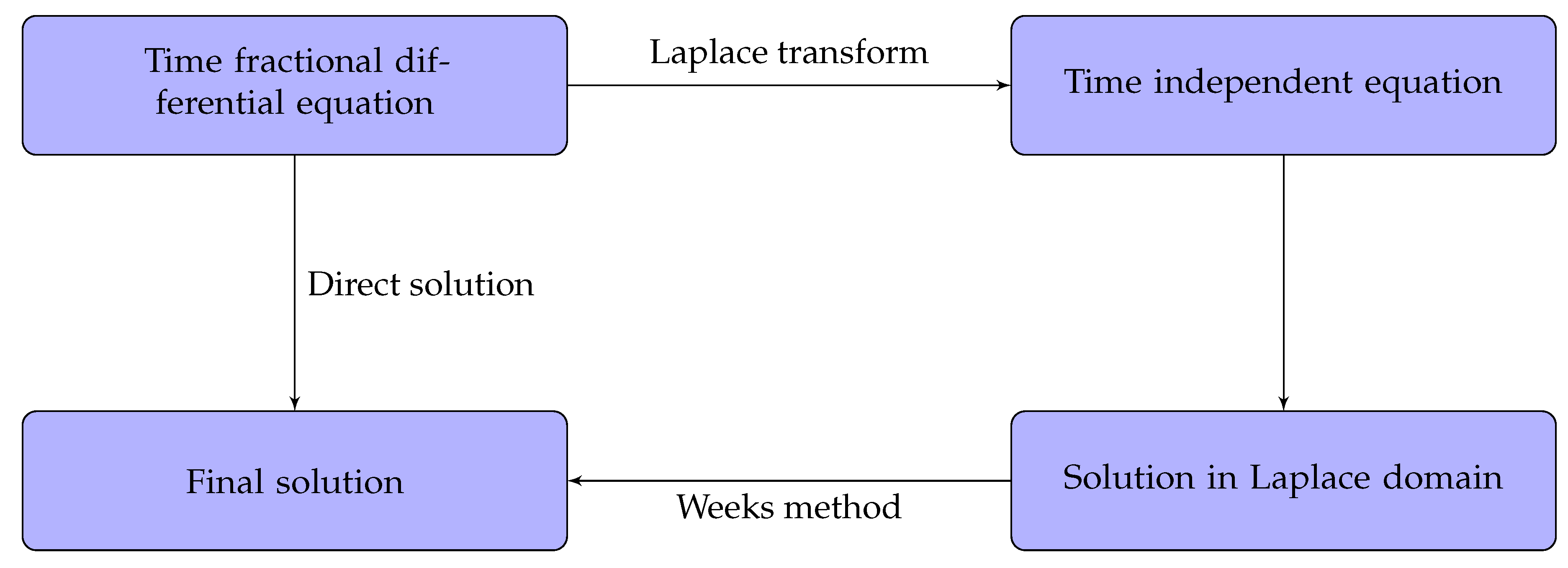
Figure 1. The flowchart of the proposed numerical method.
Symmetry 15 01214 g001
Figure 2. Laguerre polynomials.
Symmetry 15 01214 g002
Figure 3. (a) The plot of exact (Esol) and numerical (Nsol) solutions of Example 1. (b) The plot shows the AE, RE, and the E e s t for various values of N at t = 1 corresponding to Example 1. (c) The plot shows the AE, RE, and E e s t for various values of t at N = 200 corresponding to Example 1. It is observed that the theoretical results are in agreement with the computed results.
Symmetry 15 01214 g003aSymmetry 15 01214 g003b
Figure 4. (a) The plot of exact (Esol) and numerical (Nsol) solutions of Example 2. (b) The plot shows the AE, RE, and the E e s t for various values of N at t = 1 corresponding to Example 2. (c) The plot shows the AE, RE, and E e s t for various values of t at N = 200 corresponding to Example 2. It is observed that the theoretical results are in agreement with the computed results.
Symmetry 15 01214 g004
Figure 5. (a) The plot of exact (Esol) and numerical (Nsol) solutions of Example 3. (b) The plot shows the AE, RE, and E e s t for various values of N at t = 1 corresponding to Example 3. (c) The plot shows the AE, RE, and E e s t for various values of t at N = 220 corresponding to Example 3. It is observed that the theoretical results are in agreement with the computed results.
Symmetry 15 01214 g005
Figure 6. (a) The plot of exact (Esol) and numerical (Nsol) solutions of Example 4. (b) The plot shows the AE, RE, and E e s t for various values of N at t = 1 corresponding to Example 4. (c) The plot shows the AE, RE, and E e s t for various values of t at N = 220 corresponding to Example 4. It is observed that the theoretical results are in agreement with the computed results.
Symmetry 15 01214 g006
Figure 7. (a) The plot of exact (Esol) and numerical (Nsol) solutions of Example 5. (b) The plot shows the AE, RE, E e s t for various values of N at t = 1 corresponding to Example 5. (c) The plot shows the AE, RE, and E e s t for various values of t at N = 220 corresponding to Example 5. It is observed that the theoretical results are in agreement with the computed results.
Symmetry 15 01214 g007
Table 1. The numerical results corresponding to example 1.
( ρ , β ) N AE RE E est
( 0.34538 ,   26.419 ) 201.8035  ×   10 4 3.9733  ×   10 4 2.1213  ×   10 2
( 0.34538 ,   34.139 ) 302.4871  ×   10 4 5.4792  ×   10 4 1.5070  ×   10 2
( 0.55823 ,   7.6713 ) 508.2630  ×   10 6 1.8204  ×   10 5 9.6074  ×   10 3
( 0.55823 ,   10.891 ) 806.0354  ×   10 6 1.3296  ×   10 5 6.3258  ×   10 3
( 0.55823 ,   18.286 ) 1504.9259  ×   10 6 1.0852  ×   10 5 3.5762  ×   10 3
( 0.34538 ,   14.911 ) 2004.1822  ×   10 6 9.2136  ×   10 6 2.7660  ×   10 3
( 0.34538 ,   17.936 ) 2502.4210  ×   10 6 5.3336  ×   10 6 2.2599  ×   10 3
( 0.34538 ,   20.627 ) 3004.5779  ×   10 7 1.0085  ×   10 6 1.9116  ×   10 3
( 0.34538 ,   20.627 ) 4005.7410  ×   10 7 1.2648  ×   10 6 1.6436  ×   10 3
( 0.17873 ,   20.627 ) 8001.8042  ×   10 7 3.9748  ×   10 7 9.8380  ×   10 4
Table 2. The numerical results corresponding to example 2.
( ρ , β ) N AE RE E est
( 0.56672 ,   4.0034 ) 201.2757  ×   10 4 3.2451  ×   10 4 4.7261  ×   10 3
( 0.73322 ,   7.6713 ) 406.7695  ×   10 6 1.7220  ×   10 5 1.8397  ×   10 3
( 0.61508 ,   9.0014 ) 605.0217  ×   10 6 1.2774  ×   10 5 1.0649  ×   10 3
( 0.73322 ,   12.979 ) 801.8286  ×   10 6 4.6516  ×   10 6 7.2735  ×   10 4
( 0.56672 ,   12.172 ) 1001.3060  ×   10 6 3.3223  ×   10 6 5.3878  ×   10 4
( 0.56672 ,   14.018 ) 1206.7202  ×   10 7 1.7095  ×   10 6 4.2151  ×   10 4
( 0.73322 ,   19.830 ) 1406.1228  ×   10 7 1.5575  ×   10 6 3.4158  ×   10 4
( 0.56672 ,   17.936 ) 1604.7414  ×   10 7 1.2061  ×   10 6 2.8644  ×   10 4
( 0.56672 ,   19.456 ) 1803.5444  ×   10 7 9.0163  ×   10 7 2.4342  ×   10 4
( 0.56672 ,   20.627 ) 2001.3183  ×   10 9 3.3536  ×   10 9 2.1308  ×   10 4
[36] 6.1390  ×   10 7
Table 3. The numerical results corresponding to example 3.
( ρ , β ) N AE RE E est
( 1.8239 ,   3.4139 ) 201.9976  ×   10 4 4.3539  ×   10 5 1.4882  ×   10 2
( 1.6340 ,   4.5250 ) 404.6340  ×   10 5 1.0100  ×   10 5 6.1742  ×   10 3
( 1.7179 ,   6.9679 ) 603.5713  ×   10 6 7.7836  ×   10 7 3.6354  ×   10 3
( 1.6909 ,   8.7446 ) 801.2002  ×   10 5 2.6159  ×   10 6 2.4726  ×   10 3
( 1.7129 ,   10.831 ) 1004.1455  ×   10 6 9.0352  ×   10 7 1.8310  ×   10 3
( 1.6340 ,   11.004 ) 1203.3696  ×   10 6 7.3441  ×   10 7 1.4324  ×   10 3
( 1.7715 ,   15.045 ) 1401.6198  ×   10 6 3.5304  ×   10 7 1.1596  ×   10 3
( 1.6653 ,   14.784 ) 1601.4706  ×   10 6 3.2052  ×   10 7 9.6314  ×   10 4
( 1.7094 ,   17.089 ) 1801.1823  ×   10 6 2.5768  ×   10 7 8.2130  ×   10 4
( 1.7094 ,   18.756 ) 2009.7606  ×   10 7 2.1273  ×   10 7 7.0906  ×   10 4
Table 4. The numerical results corresponding to example 4.
( ρ , β ) N AE RE E est
( 2.2739 ,   4.7660 ) 208.3012  ×   10 7 8.3012  ×   10 7 2.3953  ×   10 5
( 2.7614 ,   9.1325 ) 401.2261  ×   10 8 1.2261  ×   10 8 1.2510  ×   10 6
( 2.5096 ,   11.387 ) 604.0476  ×   10 10 4.0476  ×   10 10 2.1214  ×   10 7
( 2.5764 ,   14.489 ) 807.6084  ×   10 11 7.6084  ×   10 11 5.9160  ×   10 8
( 2.6809 ,   17.953 ) 1008.8868  ×   10 11 8.8868  ×   10 11 2.1932  ×   10 8
( 2.5222 ,   19.515 ) 1201.4327  ×   10 11 1.4327  ×   10 11 9.6073  ×   10 9
( 2.5222 ,   22.186 ) 1401.2495  ×   10 11 1.2495  ×   10 11 4.8024  ×   10 9
( 2.5222 ,   24.556 ) 1605.7061  ×   10 12 5.7061  ×   10 12 2.6232  ×   10 9
( 2.2739 ,   24.556 ) 1806.3372  ×   10 13 6.3372  ×   10 13 1.5543  ×   10 9
( 1.9871 ,   23.190 ) 2001.9100  ×   10 12 1.9100  ×   10 12 1.0129  ×   10 9
( 1.9850 ,   24.556 ) 2201.0096  ×   10 12 1.0096  ×   10 12 6.8743  ×   10 10
Table 5. The numerical results corresponding to example 5.
( ρ , β ) N AE RE E est
( 2.7302 ,   1.1153 ) 209.8946  ×   10 5 1.6140  ×   10 4 9.8357  ×   10 3
( 2.7302 ,   1.8667 ) 402.0725  ×   10 5 3.3806  ×   10 5 3.7709  ×   10 3
( 2.7302 ,   2.4671 ) 604.7066  ×   10 6 7.6774  ×   10 6 2.2084  ×   10 3
( 2.7302 ,   2.4671 ) 803.3449  ×   10 6 5.4562  ×   10 6 1.7700  ×   10 3
( 2.7302 ,   2.4671 ) 1002.8179  ×   10 6 4.5966  ×   10 6 1.4797  ×   10 3
( 2.7302 ,   2.4671 ) 1207.9360  ×   10 7 1.2945  ×   10 6 1.2782  ×   10 3
( 2.7302 ,   2.4671 ) 1406.6768  ×   10 7 1.0891  ×   10 6 1.1295  ×   10 3
( 2.7302 ,   2.4671 ) 1601.3086  ×   10 6 2.1346  ×   10 6 1.0147  ×   10 3
( 2.7302 ,   2.4671 ) 1801.6979  ×   10 7 2.7695  ×   10 7 9.2328  ×   10 4
( 2.7302 ,   2.4671 ) 2008.1590  ×   10 7 1.3309  ×   10 6 8.4849  ×   10 4
Disclaimer/Publisher’s Note: The statements, opinions and data contained in all publications are solely those of the individual author(s) and contributor(s) and not of MDPI and/or the editor(s). MDPI and/or the editor(s) disclaim responsibility for any injury to people or property resulting from any ideas, methods, instructions or products referred to in the content.