Daily Semiparametric GARCH Model Estimation Using Intraday High-Frequency Data

Abstract

The GARCH model is one of the most influential models for characterizing and predicting fluctuations in economic and financial studies. However, most traditional GARCH models commonly use daily frequency data to predict the return, correlation, and risk indicator of financial assets, without taking data with other frequencies into account. Hence, financial market information may not be sufficiently applied to the estimation of GARCH-type models. To partially solve this problem, this paper introduces intraday high-frequency data to improve estimation of the volatility function of a semiparametric GARCH model. To achieve this objective, a semiparametric volatility proxy model was proposed, which includes both symmetric and asymmetric cases. Under mild conditions, the asymptotic normality of estimators was established. Furthermore, we also discuss the impact of different volatility proxies on estimation precision. Both the simulation and empirical results showed that estimation of the volatility function could be improved by the introduction of high-frequency data.

1. Introduction

The GARCH model has been widely applied in the study of financial volatility since the seminal papers of Engle [1] and Bollerslev [2]. Since then, lots of extended GARCH models have been proposed to deal with certain types of financial time series. GARCH models can be roughly divided into two types: symmetric GARCH models and asymmetric GARCH models. A symmetric GARCH model assumes that the response of the conditional variance (volatility) to shocks is only a function of the shock intensity, with no relation to the sign of the shock. An asymmetric GARCH model assumes that the response of the conditional variance (volatility) to shocks depends on both the intensity and sign (direction) of the shock. For more details, one can refer to [3,4,5,6,7,8,9,10,11].

Commonly, for both symmetric and asymmetric GARCH models, estimations usually need certain specifications for volatility function or distributional assumptions. However, such specifications and distribution assumptions could be restrictive in practice. To solve this problem, nonparametric or semiparametric ARCH/GARCH models have been proposed, see [12,13,14,15,16,17]. Compared with parametric GARCH-type models, these models are more flexible and have no restrictive function specifications and distribution assumptions. Due to their flexibility, nonparametric or semiparametric ARCH/GARCH models have been widely investigated. While most of the existing studies have focused on daily sequences and few of them have adopted information from high-frequency data. Consequently, financial market data have not been sufficiently used.

With the development of electronic trading systems, intraday high-frequency data can be obtained easily. Such data contain a lot of useful information, which can be applied to improve the estimation of daily models. Following this point, Visser [18] proposed a method to estimate the daily parametric GARCH model with high-frequency data based on the framework of the volatility proxy model. Most existing results following Visser [18] mainly focus on parametric GARCH-type models, such as [19,20,21,22,23,24]. It has been shown that asymmetric/symmetric GARCH model estimation can obviously be improved by introducing intraday high-frequency data. Liang et al. [25] utilized high-frequency data to study the estimation of the daily nonparametric ARCH model. As with cases of the parametric GARCH model, they found that the estimation of the nonparametric ARCH model could be significantly improved by using intraday high-frequency data. Their framework gave an insight into studying other nonparametric or semiparametric GARCH models. It is quite straightforward to extend the work of Liang et al. [25] to nonparametric or semiparametric GARCH models. For simplicity, this paper introduces the use of high-frequency data to estimate a semiparametric GARCH model proposed by Yang [26], which has extensive applications in practice.

The paper is arranged as follows. Section 2 introduces the daily semiparametric GARCH model. Section 3 proposes the estimation method and gives asymptotically normal properties. Simulations are given in Section 4 to show the performance of the estimation method under a finite sample. An empirical study is conducted in Section 5 to analyze the Shanghai Stock Index. Assumptions and proofs are in the Appendix A.

2. The Daily Semiparametric GARCH Model

2.1. The Semiparametric GARCH Model

Motivated by asymmetric GARCH models and nonparametric models, let $\left\{Y_t\right\}$ be a daily return series, Yang [26] introduced the followed semiparametric GARCH model to describe the conditional volatility of $\left\{Y_t\right\}$:

$$\begin{array}{c}\hfill \begin{array}{c}{Y}_t={\sigma }_t{\xi }_t,\hfill \\ {\sigma }_t^2=g\left\{{\displaystyle \sum _{j=1}^t}{\alpha }^{j-1}v(Y_{t-j};\eta )\right\},t=1,2,\cdots ,\hfill \end{array}\end{array}$$

(1)

where ${\left\{{\xi }_t\right\}}_{t=0}^{\infty }$ are i.i.d. random variables independent of $Y_0$ satisfying $E\left({\xi }_t\right)=0$, $E\left({\xi }_t^2\right)=1$, and $E\left({\xi }_t^4\right)=m_4<+\infty$, where ${\left\{{\sigma }_t^2\right\}}_{t=0}^{\infty }$ denotes the conditional volatility series such that ${\sigma }_t^2=\mathrm{var}(Y_t\left|Y_{t-1},Y_{t-2},\cdots )\right.$; the function g is some unknown smooth non-negative link function defined on $R_{+}=[0,+\infty ]$, $\alpha \in (0,1)$; ${\left\{v(y;\eta )\right\}}_{\eta \in H}$ is a known family of non-negative functions, continuous in y and twice continuously differentiable in the parameter $\eta \in H$, where $H=[{\eta }_1,{\eta }_2]$ is a compact interval with ${\eta }_1<{\eta }_2$. The model in (1) contains many symmetric models and asymmetric models as special cases. A case in point is that when $g\left(x\right)=\beta x+w/(1-\alpha )$ and $v(y;\eta )=y^2+\eta y^2{1}_{(y<0)}$, the model in (1) is reduced to the GJR model (an asymmetric model).

As in Yang’s work [26], we define

$$U_t=\sum _{j=0}^t{\alpha }^{j}v(Y_{t-j};\eta ),t=1,2,\cdots ,$$

(2)

for convenience and, then, the model in (1) can be transformed as follows:

$$Y_t=g^{1/2}\left(U_{t-1}\right){\xi }_t,{\sigma }_t^2=g\left(U_{t-1}\right),t=1,2,\cdots ,$$

(3)

where the process ${\left\{U_t\right\}}_{t=0}^{\infty }$ satisfies the Markovian equation,

$$U_t=\alpha U_{t-1}+v(g^{1/2}\left(U_{t-1}\right){\xi }_t;\eta ),t=1,2,\cdots .$$

(4)

Therefore, the model in (3) can be rewritten as

$$Y_t^2=g\left(U_{t-1}\right)+g\left(U_{t-1}\right)({\xi }_t^2-1).$$

(5)

From (5), it follows that

$$E\left(Y_t^2\left|U_{t-1}=u\right.\right)=g\left(u\right),\mathrm{var}\left(Y_t^2\left|U_{t-1}=u\right.\right)=g^2\left(u\right)(m_4-1),\mathrm{and}{m}_4=E{\xi }_t^4.$$

(6)

For the semiparametric GARCH(1, 1) model (1), we need to estimate the unknown link function $g\left(u\right)$ and the parameters $\alpha$, $\eta$. We state the estimation method in Section 3.

2.2. The Semiparametric Volatility Proxy Model

Following Visser [18], to introduce high-frequency data, we proposed a semiparametric scaling model by normalizing the trading day into a unit time interval:

$$Y_t\left(m\right)=g^{1/2}\left(U_{t-1}\right){\xi }_t\left(m\right),0\le m\le 1,{\sigma }_t^2=g\left(U_{t-1}\right),t=1,2,\cdots ,$$

(7)

where $U_t$ is defined in (2), $Y_t\left(m\right)$ indicates the continuous-time intraday log-return process on day t, and ${\xi }_k\left(m\right)$ and ${\xi }_l\left(m\right)$, where $k\ne l$, denote the standard noise processes on different days. These values are assumed to be independent and to follow the same probability distribution. When $m=1$, we have

$$Y_t=Y_t\left(1\right),{\xi }_t={\xi }_t\left(1\right),E{\xi }_t^2\left(1\right)=1$$

(8)

and the model in (7) reduces to the model in (3). It is easy to see that the model in (7) and the model in (3) share the same volatility function and $U_t$ structure, while the model in (7) introduces the intraday high-frequency information, $Y_t\left(m\right)$. Hence, it is expected to obtain a more precise estimation of volatility based on (7). However, the frequencies between $Y_t\left(m\right)$ and $U_t$ are inconsistent, and the model in (7) cannot be estimated directly. To estimate the volatility function, we further introduced a volatility proxy model.

Let $H_t$ be a function of $Y_t\left(m\right)$ with the positive homogeneity property, namely

$$H\left(s{Y}_t\left(m\right)\right)=sH\left(Y_t\left(m\right)\right)>0,fors>0.$$

(9)

Following Visser [18], $H_t$ is named as the volatility proxy. A frequently used volatility proxy is the daily realized volatility, which is given by the following:

$$H_t=R{V}_t=\sqrt{\sum _k^{ }{(r_{t,k}-r_{t,k-1})}^2},$$

(10)

where $r_{t,k}$ denotes the return over the kth intraday interval on day t. Based on (7), the homogeneity indicates that

$$H\left(Y_t\left(m\right)\right)=g^{1/2}\left(U_{t-1}\right)H\left({\xi }_t\left(m\right)\right).$$

Denote

$$\begin{array}{ccc}& & H_t\equiv H\left(Y_t\left(m\right)\right),Z_{Ht}\equiv H\left({\xi }_t\left(m\right)\right),{\mu }_{2H}=E{Z}_{Ht}^2,\hfill \\ & & {\xi }_{Ht}=Z_{Ht}/\sqrt{{\mu }_{2H}},g_H\left(u\right)=g\left(u\right){\mu }_{2H},\hfill \end{array}$$

(11)

then we can obtain the following semiparametric volatility proxy model:

$$H_t=g_H^{1/2}\left(U_{t-1}\right){\xi }_{Ht},{\sigma }_t^2=g_H\left(U_{t-1}\right),t=1,2,\cdots ,$$

(12)

where $E\left(H_t^2\right|U_{t-1})=g_H\left(U_{t-1}\right)$, $g_H\left(u\right)=g\left(u\right){\mu }_{2H}$, and $E{\xi }_{Ht}^2=1$. In the model in (12), the link function $g_H\left(u\right)$, the parameters $\alpha$, $\eta$, and a new constant ${\mu }_{2H}$ need to be estimated. When $H_t=|Y_t\left(1\right)|=|Y_t|$, $E\left(H_t^2\right|Y_{t-1})=g_H\left(Y_{t-1}\right)$ reduces to $E\left(Y_t^2\right|Y_{t-1})=g\left(Y_{t-1}\right)$, which means that only the daily information, $Y_t$, is adopted for estimation. Consequently, (12) includes the traditional daily model in (3) as a special case. Moreover, the frequencies of different variables in (12) are unified through the volatility proxy, hence, the model in (12) can be easily estimated.

3. Volatility Function Estimation

3.1. Estimation When Parameters Are Known

In this section, we suppose the parameters $\alpha$, $\eta$ are known first and discuss the estimation of the volatility function $g(·)$ in (12). In practice, we can observe the ${\left\{Y_t\right\}}_{t=1}^n$ and calculate ${\left\{H_t\right\}}_{t=1}^n$ based on a discrete intraday high-frequency sequence. Define the following:

$$V=\left(\begin{array}{c}{V}_2\\ V_3\\ \cdots \\ V_n\end{array}\right)=\left(\begin{array}{c}{H}_2^2\\ H_3^2\\ \cdots \\ H_n^2\end{array}\right),Z=\left(\begin{array}{cc}1& \frac{U_1-u}{h}\\ 1& \frac{U_2-u}{h}\\ \cdots & \cdots \\ 1& \frac{U_{n-1}-u}{h}\end{array}\right),$$

where $E_1=(1,0)$, $E_2=(0,1)$, $W=\mathrm{diag}\{\frac{1}{n}{K}_h(U_1-u),\dots ,\frac{1}{n}{K}_h(U_{n-1}-u)\}$, $K_h(·)=\frac{1}{h}K\left(\frac{·}{h}\right)$ for any kernel function $K(·)$ and a certain bandwidth h.

Referring to Yang [26], based on (12), the local linear estimator of $g_H\left(u\right)$ is given as

$${\widehat{g}}_H\left(u\right)=E_1{\left(Z^{\tau }WZ\right)}^{-1}{Z}^{\tau }WV.$$

(13)

From (13), we can obtain the local linear estimator $\widehat{g}\left(u\right)$ for $g\left(u\right)$ by setting $H_t=|Y_t\left(1\right)|=|Y_t|$, where no intraday high-frequency information is used. Note that ${\mu }_{Z_H}=g_H\left(u\right)/g\left(u\right)$ is an unknown parameter depending on $H_t$. Following Liang [25], an estimator for ${\mu }_{Z_H}$ is defined as

$${\widehat{\mu }}_{Z_H}=\frac{1}{n-1}\sum _{t=2}^n\frac{{\widehat{g}}_H\left(U_{t-1}\right)}{\widehat{g}\left(U_{t-1}\right)},$$

(14)

where ${\widehat{g}}_H\left(U_{t-1}\right)$ and $\widehat{g}\left(U_{t-1}\right)$ can be calculated according to (13). Then, the final estimator for the volatility function, $g\left(u\right)$, introducing the intraday high-frequency information is defined by

$$\tilde{g}\left(u\right)=\frac{{\widehat{g}}_H\left(u\right)}{{\widehat{\mu }}_{Z_H}}.$$

(15)

The following theorems show that ${\widehat{g}}_H\left(u\right)$ and $\tilde{g}\left(u\right)$ behave as in the standard univariate local linear estimator and may have smaller asymptotic variance by choosing a proper volatility proxy.

Theorem 1.

Under Assumptions A1–A12, for any fixed $u\in A$ given in Assumption A3, as $nh\to \infty ,n{h}^5=O\left(1\right),$

$$\sqrt{nh}({\widehat{g}}_H\left(u\right)-g_H\left(u\right)-h^2{b}_H\left(u\right))\stackrel{D}{⟶}N(0,V_H\left(u\right))$$

where $b_H\left(u\right)={\Lambda }_{0,2}{g}_H^{\left(2\right)}\left(u\right)/2$, $V_H\left(u\right)=\left|\right|K_0^{\ast }{\left|\right|}_2^2(m_4^H-1)g_H^2\left(u\right){\phi }^{-1}\left(u\right)$, and ${\Lambda }_{0,2}$ is defined in (A4).

Theorem 2.

Under Assumptions A1–A12, for any fixed $u\in A$ given in Assumption A3, if $h\sim n^{-r}$ for some $r\in (1/4,1)$, as $n\to \infty ,$$({\widehat{\mu }}_{Z_H}-{\mu }_{Z_H})=o_p\left(n^{-\frac{1}{2}}\right)$ and

$$\sqrt{nh}(\tilde{g}\left(u\right)-g\left(u\right)-h^2\tilde{b}\left(u\right))\stackrel{D}{⟶}N(0,\tilde{V}\left(x\right)),$$

where $\tilde{b}\left(u\right)={\Lambda }_{0,2}{g}^{\left(2\right)}\left(y\right)/2$ and $\tilde{V}\left(u\right)=(m_4^H-1)\left|\right|K_0^{\ast }{\left|\right|}_2^2{g}^2\left(u\right){\phi }^{-1}\left(u\right).$

Remark 1.

In Theorem 1, when $H_t=\left|Y_t\right|$, ${\widehat{g}}_H\left(u\right)$, and $g_H\left(u\right)$ become $\widehat{g}\left(u\right)$ and $g\left(u\right)$, respectively. Hence, $b_H\left(u\right)=b\left(u\right)={\Lambda }_{0,2}{g}^{\left(2\right)}\left(u\right)/2!$ and $V_H\left(u\right)=V\left(u\right)=\left|\right|K_0^{\ast }{\left|\right|}_2^2(m_4-1)g^2\left(u\right){\phi }^{-1}\left(u\right)$. Note that the estimator, $\widehat{g}\left(u\right)$, does not use high-frequency information.

Remark 2.

In Theorem 2, the revised estimator, $\tilde{g}\left(u\right)$, continues to have the same bias term as $\widehat{g}\left(u\right)$, while the asymptotic variance term is different. The main difference in asymptotic variance between $\widehat{g}\left(u\right)$ and $\tilde{g}\left(u\right)$ lies in that the previous term $(m_4-1)$ becomes $(m_4^H-1)$ after introducing high-frequency information. Consequently, a smaller $m_4^H$ will lead to smaller asymptotic variance in $\tilde{g}\left(u\right)$. Therefore, one can choose a proper volatility proxy by comparing it to the value of $m_4^H$, which is helpful in obtaining a more precise function estimator.

In practice, $m_4^H=c·E{H}_t^4/{\left(E{H}_t^2\right)}^2$ and $c={\left[E\left(g\left(U_{t-1}\right)\right)\right]}^2/E\left[g^2\left(U_{t-1}\right)\right]$. Let

$$\begin{array}{c}\hfill m_4^{H\ast }=E{H}_t^4/{\left(E{H}_t^2\right)}^2.\end{array}$$

(16)

Due to the fact that $c>0$ and $m_4^H=c·m_4^{H\ast }>0$, one can choose the optimal proxy, $H_t$, by comparing which proxy has the smallest value of $m_4^{H\ast }$.

3.2. Estimating the Parameters

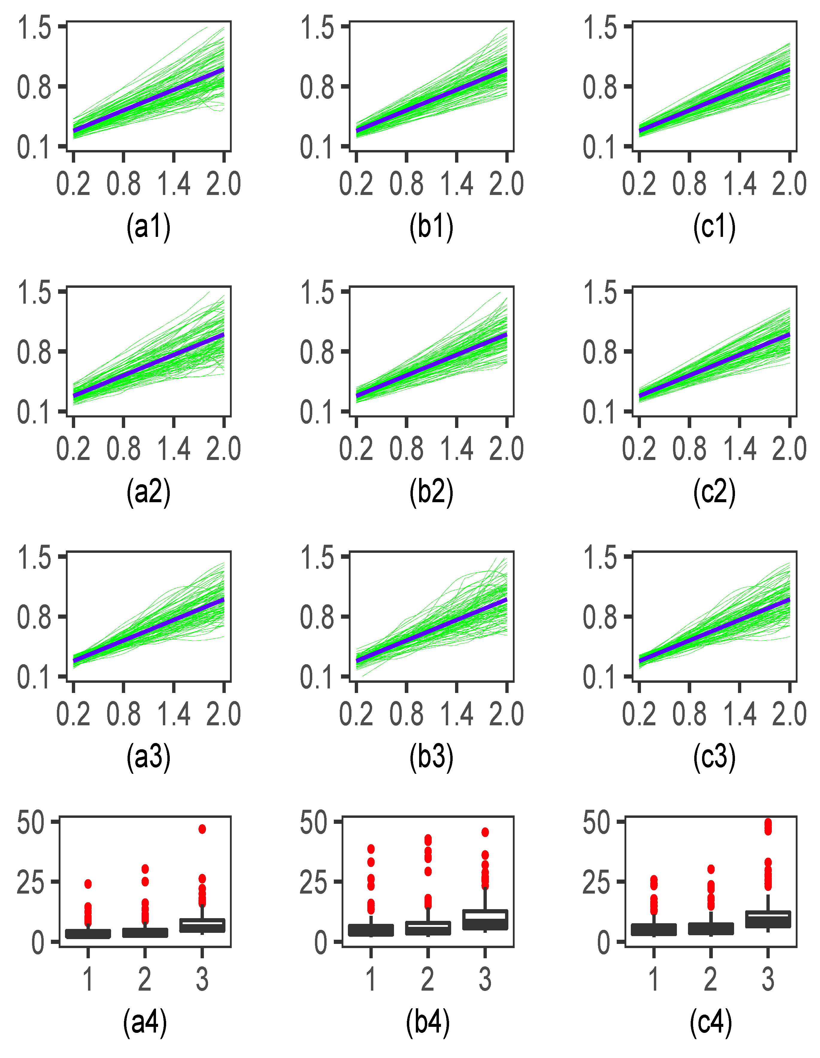
In practice, $\gamma =(\alpha ,\eta )$ is usually unknown and we discuss its estimation in this section. Without loss of generality, assume that $\gamma$ is located inside $\Gamma =[{\alpha }_1,{\alpha }_2]\times [{\eta }_1,{\eta }_2]$, where $0<{\alpha }_1<{\alpha }_2<1,-\infty <{\eta }_1<{\eta }_2<+\infty$. Let ${\gamma }^{\prime }$ be a parameter vector in $\Gamma =[{\alpha }_1,{\alpha }_2]\times [{\eta }_1,{\eta }_2]$, and consider regressing the $H_t^2$ series on $U_{{\gamma }^{\prime },t-1}$, where $U_{{\gamma }^{\prime },t}$ is given by

$$\begin{array}{c}{U}_{{\gamma }^{\prime },t}={\displaystyle \sum _{j=0}^t}{{\alpha }^{\prime }}^{j}v(Y_{t-j};{\eta }^{\prime })={\displaystyle \sum _{j=0}^t}{{\alpha }^{\prime }}^{j}v(g^{1/2}\left(U_{t-j-1}\right){\xi }_{t-j};{\eta }^{\prime }),\hfill \\ t=1,2,...,{\gamma }^{\prime }=({\alpha }^{\prime },{\eta }^{\prime })\in \Gamma .\hfill \end{array}$$

(17)

Based on $U_{{\gamma }^{\prime },t-1}$, the predictor of $H_t^2$ can be defined as

$$g_{H,{\gamma }^{\prime }}\left(u\right)=E\left(H_t^2\left|U_{{\gamma }^{\prime },t-1}=u\right.\right)$$

(18)

for any ${\gamma }^{\prime }\in \Gamma$, and the weighted mean square prediction error can be expressed as

$$L\left({\gamma }^{\prime }\right)=\underset{t\to \infty }{lim}E\{{(H_t^2-g_{H,{\gamma }^{\prime }}\left(U_{{\gamma }^{\prime },t-1}\right)\}}^2\pi \left({\tilde{U}}_{t-1}\right),$$

(19)

where $\pi (·)$ is a non-negative and continuous weight function and its compact support is contained in A, which is defined in Assumption A3. Following Yang [26], we can define a series, ${\tilde{U}}_t$:

$${\tilde{U}}_t=\sum _{j=0}^t{\alpha }_2^{j}v(g_H^{1/2}\left(U_{t-j-1}\right){\xi }_{t-j};\tilde{\eta }),t=1,2,\cdots ,$$

(20)

where $\tilde{\eta }$ is given in Assumption A4. According to A4, it is not difficult to have $\left|U_{{\gamma }^{\prime },t}\right|\le {\tilde{U}}_t,t=1,2,\cdots ,{\gamma }^{\prime }\in \Gamma$. Then, the usual deviation variance decomposition on $L\left({\gamma }^{\prime }\right)$ is performed and we obtain

$$L\left({\gamma }^{\prime }\right)=\underset{t\to \infty }{lim}E{\{g_H\left(U_{t-1}\right)-g_{H,{\gamma }^{\prime }}\left(U_{{\gamma }^{\prime },t-1}\right)\}}^2\pi \left({\tilde{U}}_{t-1}\right)+(m_4-1)\times \underset{t\to \infty }{lim}E{g}_H^2\left(U_{t-1}\right)\pi \left({\tilde{U}}_{t-1}\right).$$

(21)

From Assumption A7, $L\left({\gamma }^{\prime }\right)$ has a unique minimum point at $\gamma$ and is locally convex. Consequently, we can calculate the true parameter, $\gamma$, consistently by minimizing the prediction error of $H_t^2$ on $U_{{\gamma }^{\prime },t-1}$.

Note that $V={\left(V_t\right)}_{2\le t\le n}$, $V_t=H_t^2$, $t=2,\cdots ,n$, for each $u\in A,{\gamma }^{\prime }\in \Gamma$. Define the estimator of $g_{H,{\gamma }^{\prime }}\left(u\right)$:

$${\widehat{g}}_{H,{\gamma }^{\prime }}\left(u\right)={E^{\prime }}_1{\left({Z^{\prime }}_{{\gamma }^{\prime }}{W}_{{\gamma }^{\prime }}{Z}_{{\gamma }^{\prime }}\right)}^{-1}{Z^{\prime }}_{{\gamma }^{\prime }}{W}_{{\gamma }^{\prime }}V,$$

(22)

where

$$Z_{{\gamma }^{\prime }}={\left\{(1,\frac{U_{{\gamma }^{\prime },t}-u}{h})\right\}}_{1\le t\le n-1},W_{{\gamma }^{\prime }}=diag{\left\{\frac{1}{n}{K}_h(U_{{\gamma }^{\prime },t}-u)\right\}}_{t=1}^{n-1}.$$

Define the estimated function

$$\widehat{L}\left({\gamma }^{\prime }\right)=\frac{1}{n}\sum _{t=2}^n\{H_t^2-{\widehat{g}}_{H,{\gamma }^{\prime }}\left(U_{{\gamma }^{\prime },t-1}\right){\}}^2\pi \left({\tilde{U}}_{t-1}\right).$$

(23)

Let $\widehat{\gamma }$ be the estimator of $\gamma$. Then, $\widehat{\gamma }$ can be obtained by minimizing the above function $\widehat{L}\left(\gamma \right)$, i.e.,

$$\widehat{\gamma }=arg\underset{{\gamma }^{\prime }\in \Gamma }{min}\widehat{L}\left({\gamma }^{\prime }\right).$$

(24)

The following theorem shows the asymptotic normality of the estimator, $\widehat{\gamma }$.

Theorem 3.

Under Assumptions A1–A12, if $h\sim n^{-r}$ for some $r\in (1/5,1/4)$, then as $n\to \infty$, the $\widehat{\gamma }$ defined by (24) satisfies

$$\sqrt{n}(\widehat{\gamma }-\gamma )\to N(\mathbf{0},{\left\{{\nabla }^{2}L\left(\gamma \right)\right\}}^{-1}\Sigma {\left\{{\nabla }^{2}L\left(\gamma \right)\right\}}^{-1}),$$

where $\Sigma =4(m_4^H-1)E\left[g_H^2\left(U_1\right){\pi }^2\left({\tilde{U}}_1\right)\{\nabla g_{H,{\gamma }^{\prime }}\left(U_{{\gamma }^{\prime },1}\right)\}{\{\nabla g_{H,{\gamma }^{\prime }}\left(U_{{\gamma }^{\prime },1}\right)\}}^T\left|{}_{{\gamma }^{\prime }=\gamma }\right.\right]$.

Note that when ${\gamma }^{\prime }=\gamma$, ${\widehat{g}}_{H,{\gamma }^{\prime }}\left(u\right)$ in (18) becomes ${\widehat{g}}_H\left(u\right)$, as given in (13). Consequently, by treating the estimated value, $\widehat{\gamma }$, as the true value for the parameter, ${\widehat{g}}_H\left(u\right)$ can be approximated well by ${\widehat{g}}_{H,\widehat{\gamma }}\left(u\right)$. Then, the final estimation of the function $\tilde{g}(·)$ can be obtained based on (14) and (15).

4. Simulation

To assess the finite-sample performance of the proposed estimator, $\tilde{g}\left(u\right)$, we first need to simulate the intraday noise process, ${\xi }_t\left(m\right)$, to generate $Y_t$ and $Y_t\left(m\right)$. Following Visser [18], ${\xi }_t\left(m\right)$ is simulated by the following two processes:

$$\begin{array}{ccc}& & d{\gamma }_t\left(m\right)=-\delta ({\gamma }_t\left(m\right)-\mu )dm+{\sigma }_{\gamma }d{B}_t^{\left(2\right)}\left(m\right),\hfill \end{array}$$

(25)

$$\begin{array}{ccc}& & d{\xi }_t\left(m\right)=e^{{\gamma }_t\left(m\right)}d{B}_t^{\left(1\right)}\left(m\right),m\in [0,1].\hfill \end{array}$$

(26)

The Brownian motions $B_t^{\left(1\right)}$ and $B_t^{\left(2\right)}$ are not related. The values ${\xi }_t\left(0\right)=0$ and $\gamma \left(0\right)$ are sampled from $N(\mu ,{\sigma }_{\gamma }^2)$. We divide the unit time interval $[0,1]$ into 240 small intervals and set $\delta =1/2$, ${\sigma }_{\gamma }=1/4$, $\mu =-1/16$.

Following Liang [25], for each day, we consider three volatility proxies: the realized volatility in 5 min ($H{5}_t$), the realized volatility in 30 min ($H{30}_t$), and $|Y_t|$ (corresponding to the case without using high-frequency information). Here, $H{5}_t$ and $H{30}_t$ were calculated based on (10), and the estimation of function g was computed according to Section 3.

For model (7), we considered two asymmetric models as simulation examples:

Example 1.

$\alpha =0.5,\eta =0.1$, $\Gamma =[0.4,0.6]\times [0,0.2]$, $g\left(u\right)=0.1(2u+1)/(1-\alpha )$, and $v(y;\eta )=y^2+\eta y^2{1}_{(y<0)}$.

Example 2.

$\alpha =0.2,\eta =0.1$, $\Gamma =[0.1,0.3]\times [0,0.2]$, $g\left(u\right)=\frac{1}{\sqrt{2\pi }{\sigma }^2}{e}^{-\frac{{(u-0.5)}^2}{2{\sigma }^2}}$, where $\sigma =0.4$, and $v(y;\eta )=y^2+\eta y^2{1}_{(y<0)}$.

For the above two examples, the sample sizes were $n=300$, 600, and 900, respectively, and the replication time was 100. To obtain the estimator, $\tilde{g}\left(u\right)$, based on (15), the bandwidth was set as $1.06\times std\left(U_t\right)\times n^{-1/5}$ and the kernel function was $K\left(x\right)=0.75{(1-x^2)}_{+}.$ According to the 10% and 90% percentiles of the simulated $U_{t-1}$, the subset A in Theorem 1 was defined as $[0.2,2]$, and the grid point vector was set as $G=[0.2:0.025:2]$ for each proxy $H{5}_t$, $H{30}_t$, and $|Y_t|$.

For function estimation, we display the results in Figure 1 (Example 1) and Figure 2 (Example 2). In both figures, the green curve denotes 100 replicated estimated curves $\tilde{g}\left(G_i\right)$, and the bold black line denotes the true curve for each sample size and each proxy. The three columns correspond to the cases with $n=300$, 600, and 900 from left to right, respectively. In the first column, the subplots of (ai) $(i=1,2,3)$ are the estimated curves corresponding to the cases of the proxies $H{5}_t$, $H{30}_t$, and $|Y_t|$, respectively. Similarly, the subplots of (bi) and (ci) ($i=1,2,3$) are the estimation results for $n=600$ and 900, respectively. Subplots (a4,b4,c4) are the box plots of $m_4^{H\ast }$ in (16) for $H{5}_t$, $H{30}_t$, and $|Y_t|$ (from left to right in each subplot) under different sample sizes.

Figure 1 and Figure 2 show that the estimator under the proxy $H{5}_t$ performed best among the three proxies considered for each sample size, especially for the case with a small sample size. This was consistent with the results in subplots (a4), (b4) and (c4), which meant that, under the proxy, $H{5}_t$, the $m_4^{H\ast }$ values were generally smaller than the other proxies. The estimator under the proxy $H{30}_t$ showed more precise estimation than that of proxy $|Y_t|$. As the sample size increased, each proxy showed a better fitting performance, justifying the asymptotic normality in Theorem 2.

In addition, the mean estimation results of $\alpha$ and $\eta$ in scenarios with data of different frequencies are shown in

Table 1. The mean estimation results of $\alpha$ and $\eta$ in scenarios with data of different frequencies ($n=300$).

Example	1		2
Proxy	$\widehat{\mathbf{\alpha }}$	$\widehat{\mathbf{\eta }}$	$\widehat{\mathbf{\alpha }}$	$\widehat{\mathbf{\eta }}$
$H{5}_t$	0.4965	0.1030	0.1958	0.1013
$H{30}_t$	0.4865	0.1051	0.1991	0.0840
$\left|Y_t\right|$	0.4852	0.1055	0.2050	0.1051

,

Table 2. The mean estimation results of $\alpha$ and $\eta$ in scenarios with data of different frequencies ($n=600$).

Example	1		2
Proxy	$\widehat{\mathbf{\alpha }}$	$\widehat{\mathbf{\eta }}$	$\widehat{\mathbf{\alpha }}$	$\widehat{\mathbf{\eta }}$
$H{5}_t$	0.5003	0.1061	0.1957	0.1112
$H{30}_t$	0.4950	0.1012	0.2097	0.0991
$\left|Y_t\right|$	0.4906	0.1147	0.2041	0.1143

and

Table 3. The mean estimation results of $\alpha$ and $\eta$ in scenarios with data of different frequencies ($n=900$).

Example	1		2
Proxy	$\widehat{\mathbf{\alpha }}$	$\widehat{\mathbf{\eta }}$	$\widehat{\mathbf{\alpha }}$	$\widehat{\mathbf{\eta }}$
$H{5}_t$	0.5029	0.0969	0.1941	0.0973
$H{30}_t$	0.4983	0.1010	0.2027	0.1080
$\left|Y_t\right|$	0.5031	0.1034	0.1814	0.1013

. It is easy to find that, compared with daily proxy $|Y_t|$, the mean parameter estimation results under the high-frequency proxy were more precise. According to the simulation results, it was found that introducing intraday high-frequency data could effectively improve the estimation accuracy of the semiparametric GARCH model.

5. Empirical Study

In this section, we applied the proposed model in order to study the Shanghai Stock Index. The data spanned the period from 2 April 2004 to 2 April 2010, which consisted of 1458 days worth of high-frequency data based on a 1 min sampling frequency. The intraday log–return can be computed as

$$Y_t\left(m\right)=100[log{P}_t\left(m\right)-log{P}_{t-1}\left(1\right)],m\in [0,1],$$

(27)

where $P_t\left(m\right)$ denotes the mth intraday price on day t. First, we considered 11 different volatility proxies for each day: a 1 min realized volatility, $H{1}_t$, up to a 10 min realized volatility, $H{10}_t$, and a daily absolute return, $|Y_t|$. Here, we calculated the 1 min proxy as

$$H{1}_t=\sqrt{{\Sigma }_{k=1}^{240}{[Y_t\left(m_k\right)-Y_t\left(m_{k-1}\right)]}^2},$$

(28)

where $Y_t\left(m_k\right)$ indicates the $k^{th}$ observation in the intraday sequence, $Y_t\left(m\right)$. According to (16), the estimated values of $m_4^{H\ast }$ for proxies $|Y_t|$ and $H{1}_t-H{10}_t$ were (4.7623, 3.6370, 2.4960, 2.2525, 2.1855, 2.1993, 2.1783, 2.2584, 2.3804, 2.3623, 2.3910), where $H{6}_t$ had the smallest value. For comparison, $H{1}_t$, $H{6}_t$, $H{10}_t$, and $|Y_t|$ were considered in our study to compare the impacts of different frequencies.

To estimate the volatility function for the considered data, according to the 10% and 90% percentiles of $U_{t-1}$, we set the subset A in Theorem 1 as $[5,50]$ and the grid point vector as $G=[5:0.01:50]$. Referring to Section 3.2, we first calculated ${\left\{U_{{\gamma }^{\prime },t}\right\}}_{t=1}^{1458}$ for ${\gamma }^{\prime }$ in each estimation domain. The bandwidth was simply set as $1.06\ast std\left(U_t\right)\ast n^{-1/5}$, and the 95% confidence interval of $g\left(u\right)$ was calculated as

$$\widehat{g}\left(u\right)\pm z_{0.975}\sqrt{\frac{{∥K_0^{\ast }∥}_2^2(m_4^{H\ast }-1){\widehat{g}}^2\left(u\right)}{\widehat{\phi }\left(u\right)nh}},$$

(29)

where $z_{0.975}=1.96$, $\widehat{\phi }\left(u\right)$ is an ordinary kernel density estimator defined by Silverman (1986) [27].

The parameter estimation results are shown in

Table 4. Parameter estimation results with ASD.

Parameter	$\left|{\mathit{Y}}_{\mathit{t}}\right|$	$\mathit{H}{1}_{\mathit{t}}$	$\mathit{H}{6}_{\mathit{t}}$	$\mathit{H}{10}_{\mathit{t}}$
$\widehat{\alpha }$	0.70	0.71	0.59	0.59
	(0.1912)	(0.1431)	(0.1638)	(0.1907)
$\widehat{\eta }$	0.39	0.55	0.93	0.93
	(0.0639)	(0.0210)	(0.0331)	(0.0528)

. Figure 3 shows the function estimation results of the function $g\left(u\right)$ in the semiparameiric GARCH(1, 1) model. It was found that estimated parameters and the function under $\left|Y_t\right|$ and $H{1}_t$ showed different performances. This was not surprising as $H{1}_t$ used extremely high-frequency data, which might contain lots of noise and, hence, led to unreliable results. For the proxy $\left|Y_t\right|$, no high-frequency information was used and its results might be not that adequate. As a comparison, results under $H{6}_t$ and $H{10}_t$ seemed more similar, stable, and reasonable, which was consistent with the fact that $H{6}_t$ was optimal among different proxies.

It is of interest to compare the confidence interval under different proxies. To give an explicit demonstration, we only plotted the confidence intervals for $g\left(u_t\right)$ under $H6$ and $\left|Y_t\right|$. Figure 4 and Figure 5 show the time series plots of the estimation curves of $g\left(u_t\right)$ and its 95% confidence intervals. It can be seen that the estimated function $g\left(u_t\right)$ under $H{6}_t$ and $\left|Y_t\right|$ showed different fluctuations. In addition, the confidence intervals under $H{6}_t$ were generally narrower than those under $\left|Y_t\right|$. Therefore, the estimation results under $H{6}_t$ seemed more precise and reasonable.

6. Concluding Remarks

The volatility model has been widely applied to the study of financial markets. In this paper, we proposed a semiparametric volatility model by introducing high-frequency data. The proposed model includes many symmetric and asymmetric GARCH models as special cases. Estimators for both parameters and unknown functions were given and related limiting properties were also developed. Simulation and empirical studies implied that the estimation precision for the considered model could be effectively improved by choosing a proper volatility proxy. The work in this paper is insightful and could be used for the further study of other symmetric/asymmetric GARCH models by using intraday high-frequency data.

References

1. Engle, R.F. Autoregressive conditional heteroskedasticity with estimates of the variance of U.K. Inflation. Econometrica 1982, 50, 987–1008. [Google Scholar] [CrossRef]
2. Bollerslev, T. Generalized autoregressive conditional heteroskedasticity. J. Econom. 1986, 31, 307–327. [Google Scholar] [CrossRef] [Green Version]
3. Engle, R.F.; Lilien, D.M.; Robbins, R.P. Estimating time varying risk premia in the term structure: The ARCH-M model. Econometrica 1987, 55, 391–407. [Google Scholar] [CrossRef]
4. Nelson, D.B. Conditional heteroskedasticity in asset returns: A new approach. Economics 1991, 59, 347–370. [Google Scholar] [CrossRef]
5. Glosten, L.R.; Jagannathan, R.; Runkle, D. On the relation between the expected value and the volatility of the nominal excess return on stocks. J. Financ. 1993, 48, 1779–1801. [Google Scholar] [CrossRef]
6. Engle, R.F.; Sokalska, M.E.; Chanda, A. High frequency multiplicative component GARCH. Comput. Econ. Financ. 2005, 409. [Google Scholar] [CrossRef]
7. Liaqat, M.I.; Akgül, A.; De la Sen, M.; Bayram, M. Approximate and Exact Solutions in the Sense of Conformable Derivatives of Quantum Mechanics Models Using a Novel Algorithm. Symmetry 2023, 15, 744. [Google Scholar] [CrossRef]
8. Hasan, A.; Akgül, A.; Farman, M.; Chaudhry, F.; Sultan, M.; De la Sen, M. Epidemiological Analysis of Symmetry in Transmission of the Ebola Virus with Power Law Kernel. Symmetry 2023, 15, 665. [Google Scholar] [CrossRef]
9. Attia, N.; Akgül, A.; Alqahtani, R.T. Extension of the Reproducing Kernel Hilbert Space Method’s Application Range to Include Some Important Fractional Differential Equations. Symmetry 2023, 15, 532. [Google Scholar] [CrossRef]
10. Farman, M.; Shehzad, A.; Akgül, A.; Baleanu, D.; De la Sen, M. Modelling and Analysis of a Measles Epidemic Model with the Constant Proportional Caputo Operator. Symmetry 2023, 15, 468. [Google Scholar] [CrossRef]
11. Attia, N.; Akgül, A.; Seba, D.; Nour, A.; De la Sen, M. An Efficient Approach for Solving Differential Equations in the Frame of a New Fractional Derivative Operator. Symmetry 2023, 15, 144. [Google Scholar] [CrossRef]
12. Engle, R.F.; Ng, V.K. Measuring and testing the impact of news on volatility. J. Financ. 1993, 48, 1749–1778. [Google Scholar] [CrossRef]
13. Yang, L.; Härdle, W.; Nielsen, J. Nonparametric autoregression with multiplicative volatility and additive mean. J. Time Ser. Anal. 1999, 20, 597–604. [Google Scholar] [CrossRef] [Green Version]
14. Hafner, C. Nonlinear Time Series Analysis with Applications to Foreign Exchange Rate Volatility; Physica-Verlag: Heidelberg, Germany, 1998. [Google Scholar]
15. Carroll, R.; Härdle, W.; Mammen, E. Estimation in an additive model when the components are linked parametrically. Econom. Theory 2002, 18, 886–912. [Google Scholar] [CrossRef] [Green Version]
16. Yang, L. Finite nonparametric GARCH model for foreign exchange volatility. Commun. Stat.-Theory Methods 2000, 5–6, 1347–1365. [Google Scholar] [CrossRef]
17. Yang, L. Direct estimation in an additive model when the components are proportional. Stat. Sin. 2002, 12, 801–821. [Google Scholar]
18. Visser, M.P. Garch parameter estimation using high-frequencydata. J. Financ. Econom. 2011, 9, 162–197. [Google Scholar]
19. Huang, J.S.; Wu, W.Q.; Chen, Z.; Zhou, J.J. Robust M-estimate of GJR model with high frequency data. Acta Math. Appl. Sin. Engl. Ser. 2015, 31, 591–606. [Google Scholar] [CrossRef]
20. Wang, M.; Chen, Z.; Wang, C.D. Composite quantile regression for GARCH models using high-frequency data. Econom. Stat. 2018, 7, 115–133. [Google Scholar] [CrossRef]
21. Deng, C.; Zhang, X.; Li, Y.; Xiong, Q. Garch Model Test Using High-Frequency Data. Mathematics 2020, 8, 1922. [Google Scholar] [CrossRef]
22. Zhang, X.; Zhang, R.; Li, Y.; SL, C. LADE-based inferences for autoregressive models with heavy-tailed G-GARCH(1, 1) noise. J. Econom. 2022, 227, 228–240. [Google Scholar] [CrossRef]
23. Li, L.; Zhang, X.; Deng, C.; Li, Y. Quasi Maximum Exponential Likelihood Estimation of GARCH Model Based on High Frequency Data. Acta Math. Appl. Sin. Engl. Ser. 2022, 45, 652–664. [Google Scholar]
24. Li, L.; Zhang, X.; Li, Y. Daily GARCH Model Estimation Using High Frequency Data. J. Guangxi Norm. Univ. (Nat. Sci. Ed.) 2021, 39, 68–78. [Google Scholar]
25. Liang, X.; Zhang, X.; Li, Y.; Deng, C. Daily nonparametric ARCH(1) model estimation using intraday high frequency data. AIMS Math. 2021, 6, 3455–3464. [Google Scholar] [CrossRef]
26. Yang, L. A semiparametric GARCH model for foreign exchange volatility. J. Econom. 2006, 130, 365–384. [Google Scholar] [CrossRef]
27. Silverman, B.W. Density Estimation; Chapman & Hall: London, UK, 1986. [Google Scholar]
28. Fan, J.; Yao, Q. Nonlinear Time Series: Nonparametric and Parametric Methods; Springer: New York, NY, USA, 2003. [Google Scholar]
29. Härdle, W.; Tsybakov, A.B.; Yang, L. Nonparametric vector autoregression. J. Stat. Plan. Inference 1998, 68, 221–245. [Google Scholar]
30. Yoshihara, K. Limiting behavior of U-statistics for stationary, absolutely regular processes. Probab. Theory & Relat. Fields 1976, 35, 237–252. [Google Scholar]
Figure 1. The subplots of (ai,bi,ci) ( i = 1 , 2 , 3 ) are the estimated curves for g ˜ ( G i ) (green lines) and the true function curve of g ( G i ) (bold black line) for different sample sizes and different proxies. The subplots (a4,b4,c4) are the box plots of m 4 H in (16) for H 5 t , H 30 t , and | Y t | (from left to right in each subplot) under different sample sizes.
Symmetry 15 00908 g001
Figure 2. The subplots of (ai,bi,ci) ( i = 1 , 2 , 3 ) are the estimated curves for g ˜ ( G i ) (green lines) and the true function curve of g ( G i ) (bold black line) for different sample sizes and different proxies. The subplots (a4,b4,c4) are the box plots of m 4 H in (16) for H 5 t , H 30 t , and | Y t | (from left to right in each subplot) under different sample sizes.
Symmetry 15 00908 g002
Figure 3. Estimation results of the function g ( u ) in the semiparametric GARCH model under H 1 t , H 6 t , H 10 t , and the | Y t | proxy.
Symmetry 15 00908 g003
Figure 4. Estimation and 95% confidence interval of the function g ( u ) in the semiparametric GARCH model under H 6 t and the | Y t | proxy.
Symmetry 15 00908 g004
Figure 5. Estimation and 95% confidence interval of the function g ( u ) in the semiparametric GARCH model under H 6 t and the | Y t | proxy.
Symmetry 15 00908 g005