1. Introduction
Air pollution refers to the presence of pollutants such as carbon monoxide (CO), ozone (O
3), nitrogen dioxide (NO
2), sulfur dioxide (SO
2), and particulate matter with a size of less than 10 microns (PM
10) in the outdoor air [
1]. These pollutants come from sources such as motor vehicles, industrial activities, open burning, and forest fires [
2]. To monitor the local air quality, authorities usually use the air pollution index (API) [
3]. When the API crosses a certain threshold, air pollution is classified as unhealthy, which implies that the air is dangerous to breathe and harmful to human health [
4]. In addition to affecting health, unhealthy air pollution events have large social and economic impacts [
5,
6,
7,
8]. For instance, such events can lead to severe health problems such as respiratory diseases, cardiovascular diseases, and skin allergies [
9,
10]. In addition, public movement is restricted, causing people to stay indoors, masks to be worn when outside, and schools to be closed [
11]. Consequently, unhealthy air pollution events reduce the national income due to partial business operations, a decline in tourist activity, increased national health costs, and decreased national productivity [
12]. Therefore, examining unhealthy air pollution events is vital to provide a clearer understanding of the air pollution data and determine the future potential risks.
In multivariate modeling, copula functions provide a significant result for modeling the dependence structure of the random variables related to the air pollution data. This success story is due to the great flexibility in modeling the multivariate distributions that copula functions provide due to the separation between the dependence structure and the univariate distributions of the variables [
13,
14]. Previously, Sak et al. [
15] applied the
-copula to PM2.5 levels to investigate the air pollution risk. Chan and So [
16] used a Gaussian copula on multiple air pollutants to understand air pollution. Falk et al. [
17] analyzed the air pollutants in Milan, Italy, using the generalized Pareto copula. Kim et al. [
18] investigated the PM2.5 time series data in China using an asymmetric bivariate copula function comprising the mixed Frank and Gumbel copulas. Masseran and Hussain [
19] applied Gaussian and modified Joe–Clayton copulas individually for constant and dynamic cases of air pollutant variables to investigate air pollution events. In addition, He et al. [
20] employed a mixed copula model to investigate the dynamic relationship between the meteorological factors and the atmospheric pollutants in the cities of Beijing and Guangzhou, China.
In addition to the PM2.5 levels, air pollutants data, and other relevant variables (e.g., meteorological factors) that have been used in the above studies, the characteristics of a calamity such as a drought or unhealthy air pollution events can also be studied for risk monitoring and controlling purposes [
21]. Motivated by this idea, Masseran [
22] studied two characteristics of unhealthy air pollution events, namely, the duration and severity, and the result showed that the fitted Joe copula could model the dependence structure between those two variables. Furthermore, Masseran [
22] derived probability measures to plan and mitigate the risks of unhealthy air pollution events. Therefore, continuing the latter study, this study also aims to model the characteristics of unhealthy air pollution events, such as the duration, severity, and intensity.
In contrast to [
22], a new characteristic, the intensity, is studied alongside the duration and severity using copula functions. For a better understanding of the air pollution behavior, this new addition is reasonable because the severity depends on not only the duration but also the intensity [
23]. Therefore, this study focuses on determining the most appropriate bivariate copula model for each possible pair of variables, which are the (intensity, duration), (intensity, severity), and (duration, severity). To this end, a wide range of existing parametric copula models was examined in this study. In searching for the appropriate model, the information-based model comparison (AIC, BIC, log-likelihood) and non-nested model comparison (Vuong and Clarke tests) were applied.
Our study found that the appropriate bivariate copula models for modeling the distribution of the relationship pairs of the (duration, intensity), (severity, intensity), and (duration, severity) were the Tawn type 1, 180°-rotated Tawn type 1, and Joe, respectively. This result showed that the dependence structures for the pairs were skewed and asymmetric. Therefore, the obtained copulas were the most appropriate models for such non-elliptical structures. Furthermore, the obtained bivariate copula models importantly served as the basis (or building blocks) for the development of a vine copula model (a more flexible and tractable model for modeling the multivariate data using bivariate copulas) in future studies.
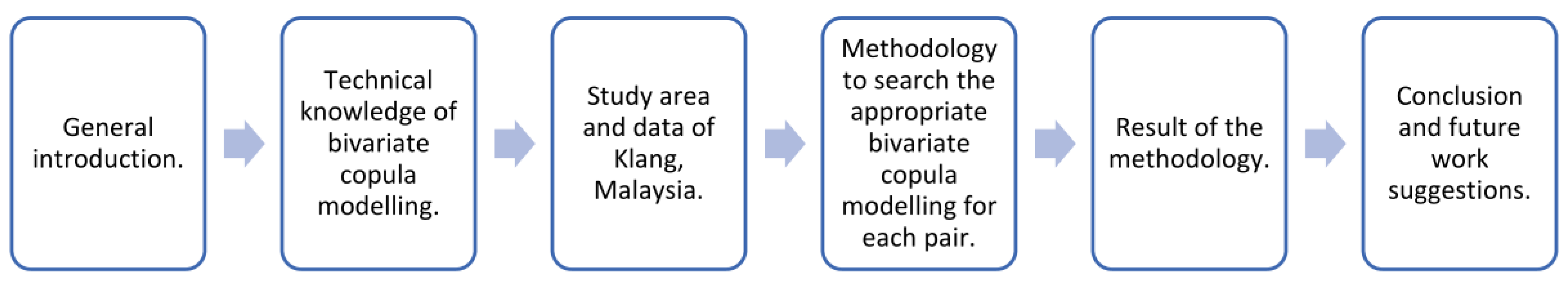
This paper is organized as follows.
Section 2 introduces a bivariate copula and its relevant properties.
Section 3 briefly covers the study area and data.
Section 4 describes the proposed methods.
Section 5, presents and discusses the results.
Section 6 ends this paper with a conclusion and some suggestions for future work.
Figure 1 illustrates a pipeline for the content of this manuscript to help readers understand the full text.
2. Bivariate Copula
Originating from Sklar’s theorem [
24], a bivariate copula
is a bivariate distribution function on the
-dimensional hypercube
with uniformly distributed marginals [
25]. To clarify, this theorem covers any arbitrary dimensionality, but this discussion focuses on the
-dimensional case. The theorem states that for a two-dimensional random vector
with a joint distribution function
and marginal distribution functions
, for
, the joint distribution function can be expressed as the following.
with the corresponding density of
where
and
are the copula and copula density, respectively. For a continuous distribution, the copula
is unique. Consequently, the corresponding copula density can be obtained by a partial differentiation, such as the following.
where
for
, which is known as the copula scale [
26].
Various bivariate copula models with unique characteristics have been proposed in the literature to model the relationship between the two random variables. Some examples are the Clayton copula, the Frank copula, and the Joe copula. To investigate the dependence properties of these bivariate copulas, the central measure of the dependence, such as Kendall’s tau, is considered. In particular, Kendall’s tau can be defined as the following.
where
and
are independently and identically distributed (i.i.d) copies of
. Since
is independent with regards to the marginal transformations, it depends only on the underlying copula. Specifically, Kendall’s tau holds that the following [
27].
The Clayton copula is useful for capturing the positive dependence of the bivariate variables, where the strength of the dependency is dictated by the Kendall’s tau correlation. With a particular rotation, this copula also can model a negative dependence structure that exists in a dataset [
28]. The bivariate Clayton copula and its density are, respectively, given below.
where
controls the degree of dependence.
In contrast, the Frank copula provides a versatile dependency measure because it can accommodate the entire range of dependencies for the positive and negative sides [
29,
30]. The bivariate Frank copula and its density are, respectively, provided below.
where
and
. Last but not least, the Joe copula can be used to describe the positive dependence among the variables [
28,
29]. In addition, the Joe copula has been proposed to address cases with a high positive correlation [
31]. To cover the negative dependence, the rotation can be applied to the Joe copula [
22]. The bivariate Joe copula is shown below.
where
. The three abovementioned copulas are classified as the Archimedean copulas with a different generator function (a unique identity of copula functions within the Archimedean copula family) [
26].
For the Archimedean copulas, such as the Clayton, Frank, and Joe copulas, Kendall’s tau also responds to their generator function
. Generally, the corresponding Kendall’s tau for an Archimedean copula is obtained using the following [
26,
32].
For the Clayton copula, its generator function is
and its Kendall’s tau is
. The generator function and Kendall’s tau for the Frank copula are, respectively, as follows.
where
is the Debye function [
25]. For the Joe copula, the generator function and Kendall’s tau are, respectively, given below.
where
is the Euler constant, and
is the digamma function [
26].
To extend the range of dependence of
, the counterclockwise rotations of the copula density
of 90°, 180°, and 270° can be used, where they are defined as
, and
, respectively [
26]. For example, using a 90° rotation, the Clayton copula can be extended to a copula with a full range of Kendall’s tau values by defining the following.
where
[
26].
3. Study Area and Data
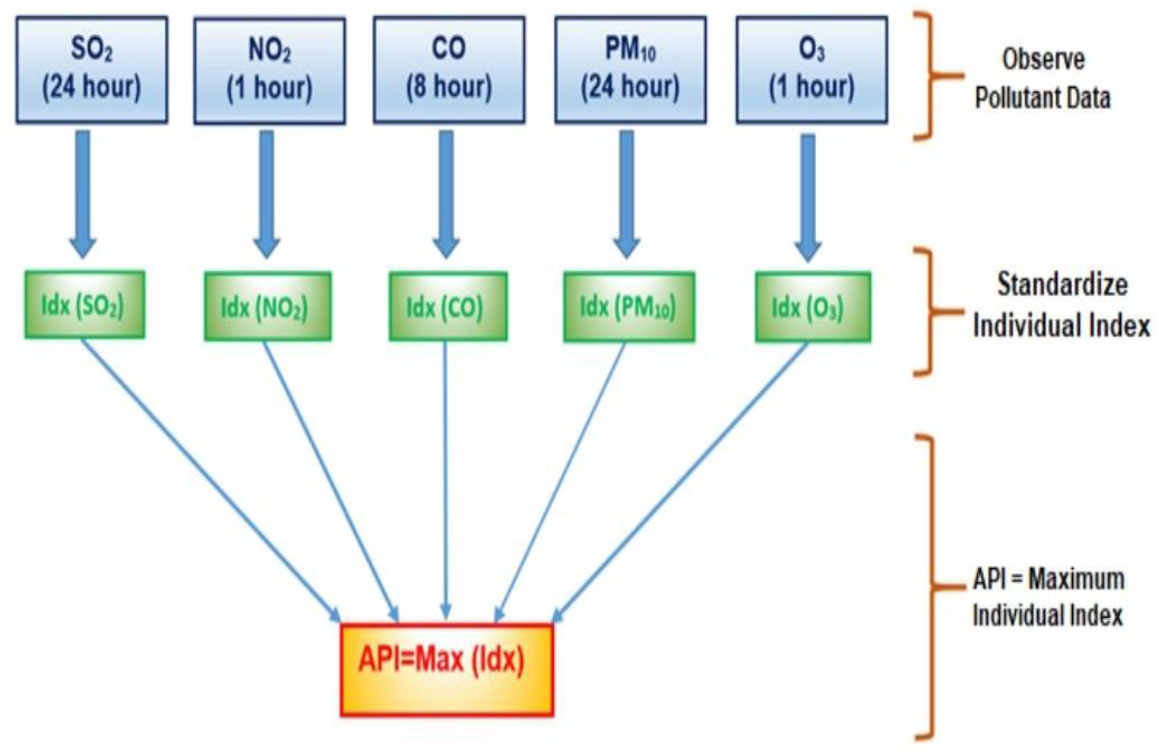
In Malaysia, the local air quality is continuously monitored by the Malaysian Department of the Environment (DOE). The DOE is responsible for collecting, supervising, and reporting the API data. To measure the API in a certain area, air quality monitoring stations were placed in strategic areas covering urban, suburban, and industrial areas. Each station records the concentration readings for the five main pollutants: carbon monoxide (CO), ozone (O3), nitrogen dioxide (NO2), sulfur dioxide (SO2), and particulate matter less than 10 microns in size (PM10). O3, CO, NO2, and SO2 are measured in the parts per million (ppm) unit mass of a contaminant, while PM10 is measured in micrograms per cubic meter ().
The API is determined based on the highest level of the five main standardized pollutants. The calculation of the standardized sub-API indices can be undertaken using the mathematical formulas provided by the DOE [
33]. The standardized sub-API value for the CO pollutant can be computed using the following equation.
The standardized sub-API value for the O
3 pollutant can be computed using the following equation.
The standardized sub-API value for the NO
2 pollutant can be computed using the following equation.
The standardized sub-API value for the SO
2 pollutant can be computed using the following equation.
The standardized sub-API value for the PM
10 pollutant can be computed using the following equation.
From these standardized individual indices, the API value at a particular time can then be determined based on the highest value among these sub-indices [
34,
35].
Figure 2 shows the process for determining the API.
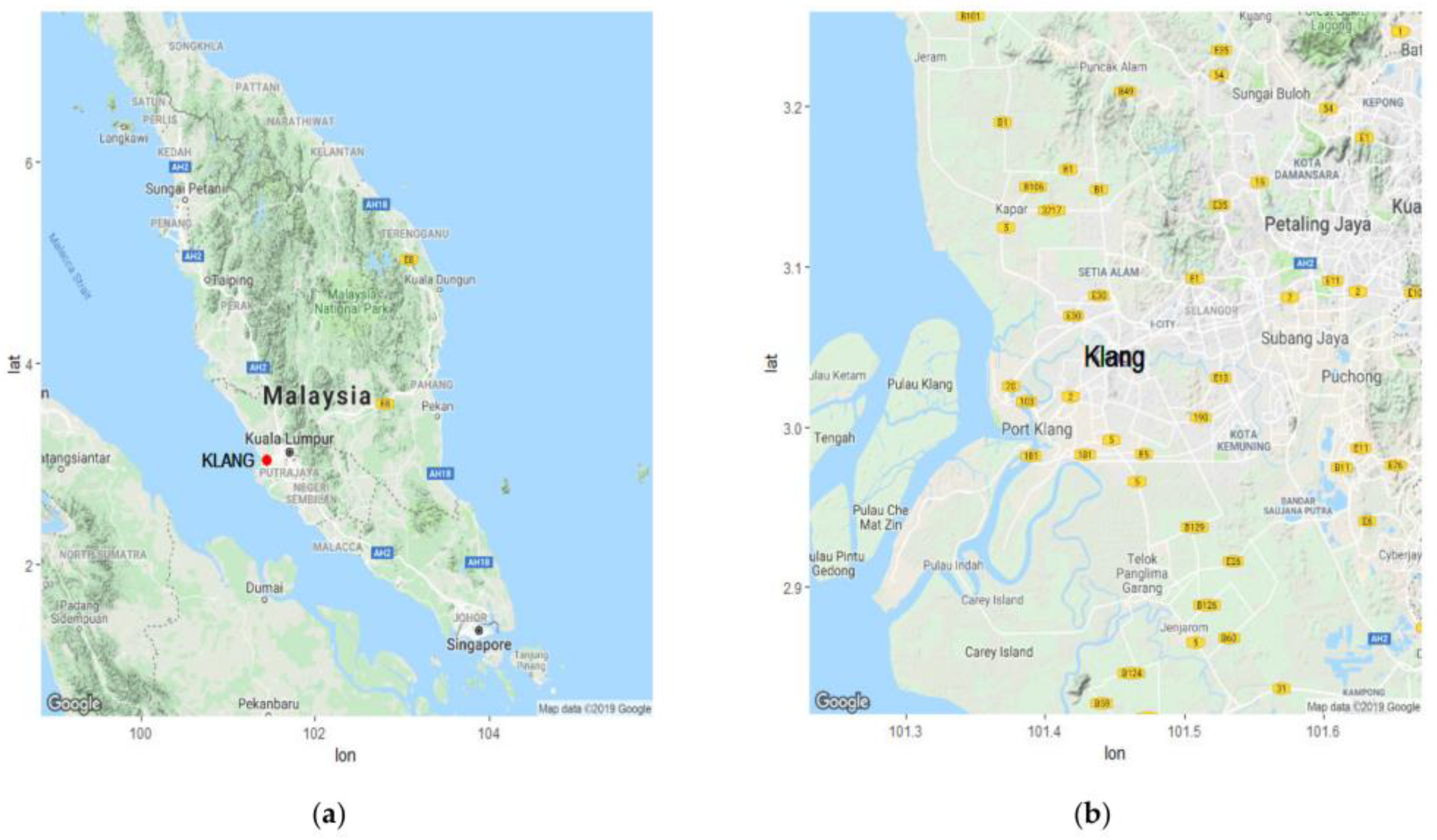
For our analysis, Klang (latitude
and longitude
), located in Peninsular Malaysia, was chosen as the study area. It is one of the largest cities in Malaysia with a dense population and a high level of economic and industrial activity, particularly in import and export trade. In addition, Klang is the 13th busiest trans-shipment and 16th busiest container port in the world [
36]. Therefore, the frequency of unhealthy air pollution events in Klang is higher compared to the other cities [
23], leading to more sample data.
Figure 3 [
37] illustrates the location of Peninsular Malaysia and Klang.
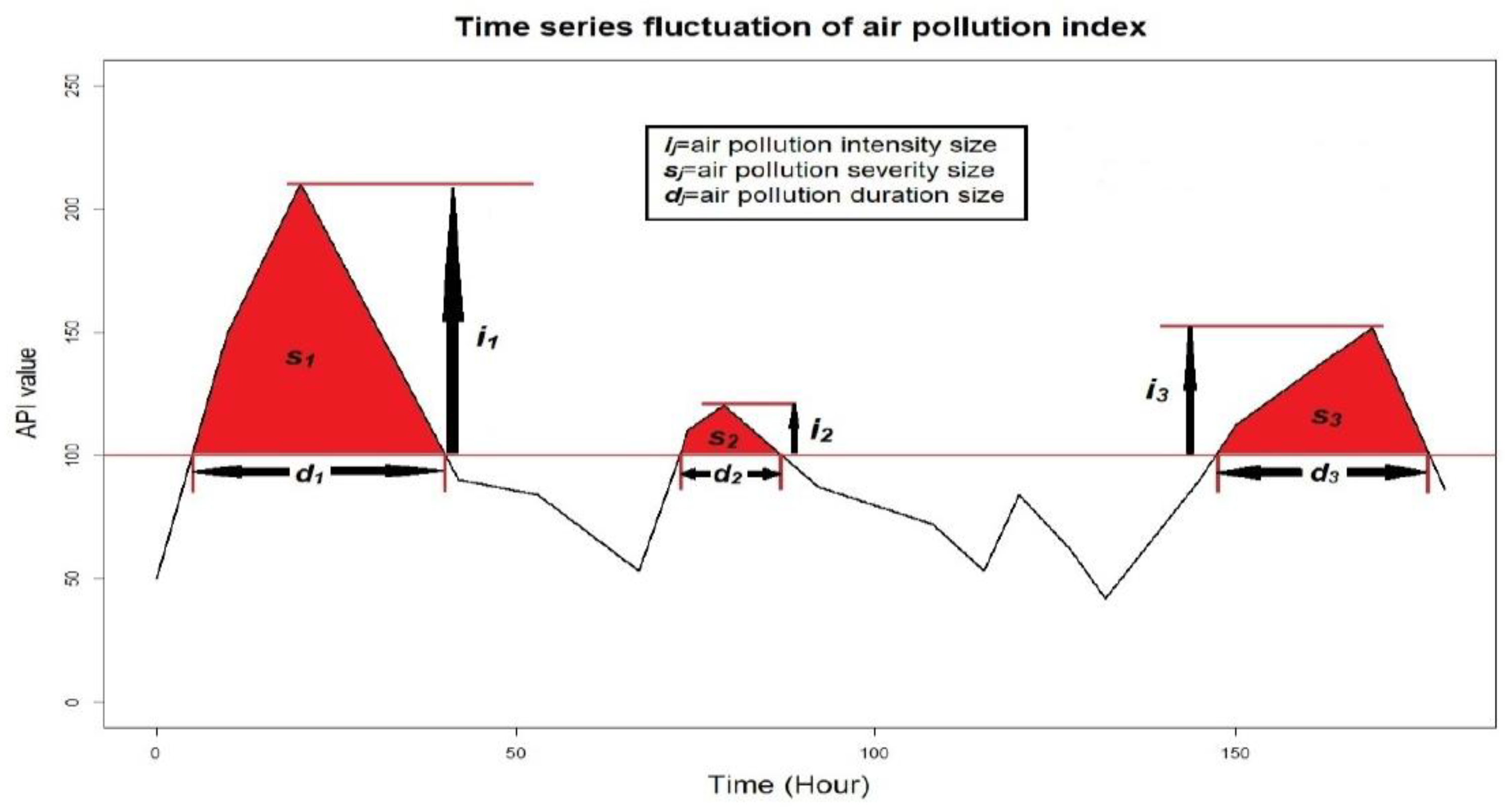
To examine the unhealthy air pollution events in Klang, its regional API data was obtained. An unhealthy air pollution event, as classified by the DOE, refers to a period when the API value exceeds 100 [
38]. Take the obtained API data as a set,
, where
is the API value along the time index
. Furthermore, let the total number of the recorded unhealthy air pollution events be
. Then, for
, the period for the
-th unhealthy air pollution event can be denoted as
. For each non-overlapping
, the duration, severity, and intensity, respectively, can be denoted as the following.
(the cardinality of the period ),
(the summation of all the API values within the period ), and
(the maximum API value within the period ).
Figure 4 provides an illustration for determining the durations, severities, and intensities of the first three air pollution events.
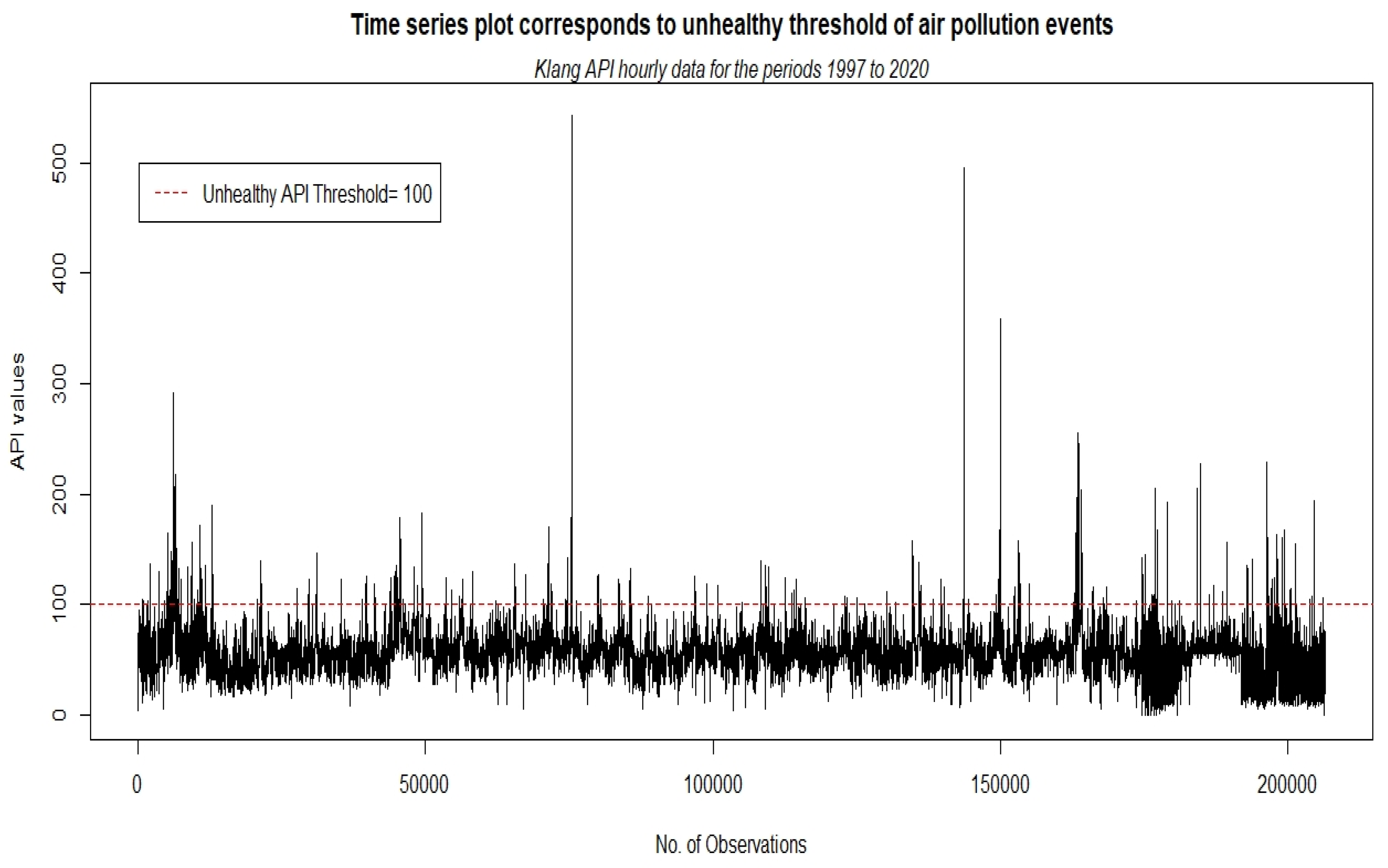
Obtained from the DOE, the hourly API data from 1 January 1997 to 31 August 2020 that were used in this study are depicted in
Figure 5. Three metrics were obtained from
Figure 5, namely, the severity, duration, and intensity. The total number of these three metrics was 301, which means that 301 unhealthy air pollution events were recorded from 1997 to 2020. Moreover, the descriptive statistics for the severity, duration, and intensity data are provided in
Table 1. The center measures (means and medians) showed a large discrepancy among the data. Furthermore, the measures of the spreads (the ranges between the minimum values and the maximum values and standard deviations) were large, showing that the data had a substantial variation, particularly the severity data. In addition, all the characteristics (severity, duration, and intensity) had a considerable skewness, with a long right tail distribution (shown by the kurtosis values).
In this study, the severity measures how severe an unhealthy air pollution event was, the duration is its time span, and the intensity is its largest magnitude. These three metrics (severity, duration, and intensity) are very dependent on each other and influence the distribution of each possible pair that will be fitted by the bivariate copula modeling. Therefore, the dependency for each pair of variables will be analyzed using a bivariate copula. The details on our methods are provided in the section below.
Figure 5.
Time series plot that corresponds to an unhealthy threshold of air pollution events.
Figure 5.
Time series plot that corresponds to an unhealthy threshold of air pollution events.
Table 1.
Descriptive statistics for the intensity, severity and duration data.
Table 1.
Descriptive statistics for the intensity, severity and duration data.
| Variable | Mean | Median | Min. Value | Max. Value | Std. Deviation | Skewness | Kurtosis |
|---|
| Intensity | 125.11 | 112 | 100 | 543 | 44.77 | 5.61 | 44.97 |
| Severity | 2241.76 | 231.27 | 100 | 36,677 | 4948.3 | 3.92 | 20.92 |
| Duration (hours) | 16.74 | 2 | 1 | 224 | 31.91 | 3.24 | 15.73 |
4. Methodology
Let
,
, and
be the sets of the duration, severity, and intensity of
unhealthy air pollution events. The focus of this study is on investigating the dependence structure among all the possible pairs of these three random variables using bivariate copula modeling (as discussed in
Section 2). Three pairs are possible, namely the (
,
), (
,
), and (
,
).
For simplicity, let
,
, and
represent the
,
, and
, respectively. First, each variable was transformed into the corresponding pseudo-copula data using an estimated probability integral transform (PIT) by setting
for
, and
. Here, an empirical distribution function was used to transform the variables, defined as the following.
where
is the
-th variable. Thus, the copula data
was obtained, where
is the copula data for the
-th variable.
Next, using the copula data , the pairwise dependencies among the variables (, , and ) were explored. For that purpose, a plot comprising the marginal histograms of the copula data, pair plots of the copula data, Kendall’s tau coefficients, and empirical contour plots of the normalized copula data were used to inspect the pairwise dependency structures.
Generally, the copula models can be classified into at least two groups, such as elliptical copulas and non-elliptical copulas. The copulas derived from an elliptical distribution are Gaussian and Student t-copulas. The other copulas are non-elliptical and have more flexibility to model asymmetric and skewed distributions. All these copula models can be applied to the characteristics of the unhealthy air pollution events, and the obtained models can provide useful information regarding their dependencies, regardless of whether they are distributed in a symmetric or asymmetric distribution.
Table 2 lists all the considered bivariate copula models in this study.
Then, the copula modeling approach was used to model the dependence structure for each pair of variables. For each pair, the parameters for each considered bivariate copula model were estimated using the maximum likelihood estimation (MLE). For the observations
where
, and
, the MLE was computed as follows.
with a likelihood function of
where
is the parameter of the possible set
that maximizes the likelihood function.
Generally, there are two ways to optimize the copula parameters, namely the MLE and the inversion of the empirical Kendall’s tau estimation. As defined above, the MLE is suitable for cases where the number of parameters is not too large (e.g., one or two). While the inversion of the empirical Kendall’s tau uses the one-to-one relationship between the tau and the copula parameter to estimate the copula parameters. However, the inversion of the empirical Kendall’s tau approach is less efficient and is not applicable to all the bivariate copula models [
27]. Only one parameter bivariate copula models and the Student
-copula can be used in the approach [
39]. Therefore, the MLE is preferable compared to the inversion of the empirical Kendall’s tau estimation.
Henceforth, for each bivariate copula model with its optimized parameters, an information-based model comparison comprised the Akaike information criteria (AIC) and Bayesian information criterion (BIC), and a log-likelihood was applied to choose the best model for each pair. Here, any bivariate copula model that obtained the highest log-likelihood and the lowest AIC and BIC was considered superior. For the observations
where
, and
, the AIC, BIC, and log-likelihood were computed as follows.
where
is the number of the bivariate copula model parameters, and [
26,
39]
For this study, the function named BiCopEstList under the R-package VineCopula was used to build these copula models and obtain all the AIC, BIC, and log-likelihood values.
In addition, the scoring of the goodness-of-fit tests based on the Vuong and Clarke tests were applied to compare the models [
40,
41,
42]. In these two tests, the best model was assumed to fit the data better than all the other models. Therefore, if model one was superior to model two, a score of one was assigned to model one. However, if model two was favored over model two, a score of −1 was assigned to model one. If the tests could not discriminate between the two compared models, nothing was assigned. Through these tests, a model that fit the data better than any other model was identified. In addition, the model with the highest score on the Vuong and Clarke tests was selected as the best model. In this study, the function BiCopVuongClarke in the R-package VineCopula was used for the computation [
39].
5. Results
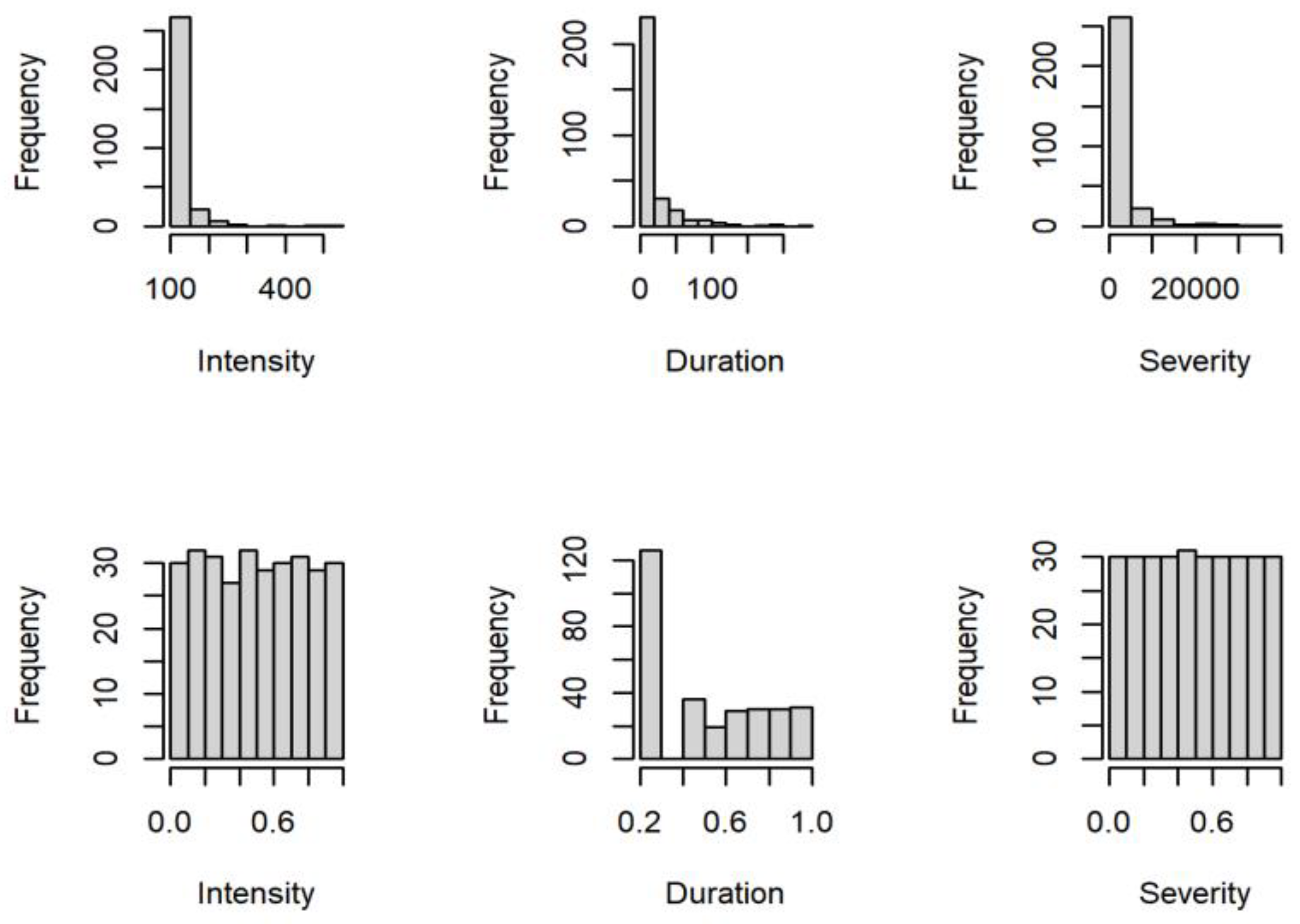
In this study, three random variables related to the characteristics of the unhealthy air pollution events, namely, the intensity, duration, and severity, were examined. Specifically, each pair of variables was modeled using a bivariate copula to describe its dependence structure. First, each original variable was transformed into a copula variable using the PIT approach. The margin histograms of the original and copula variables are illustrated in the first and second rows in
Figure 6, respectively. In
Figure 6, the marginal distributions of the copula variables seemed more uniformly distributed compared to the original variables. This comparison showed that in the copula variables, the marginal distribution effects and the dependence structure were separated to obtain more accurate and flexible modeling using the copula function.
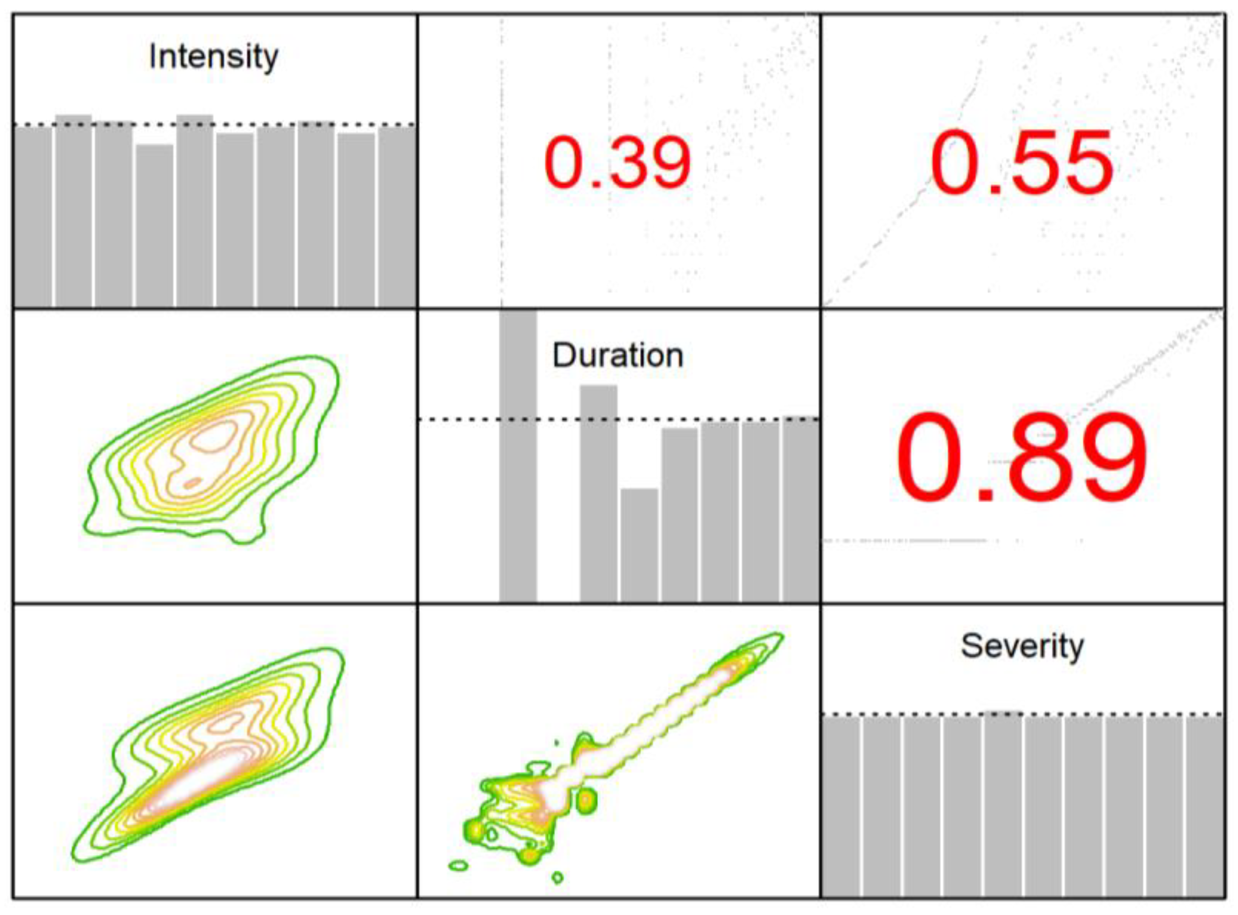
Before the copula function was applied, a pairwise dependency for each pair of copula variables was investigated using marginal histograms, pair plots, Kendall’s tau coefficients, and empirical contour plots. The obtained marginal histograms, pair plots, Kendall’s tau coefficients, and empirical contour plots for all the pairs are provided in
Figure 7. The lower left blocks of
Figure 7 located below the diagonal contain the normalized contour plots. The different colors in the empirical contour plots indicate the density of each pair of variables, where the yellowish color represents a higher density than the greenish color. As a preliminary analysis in the copula modeling, the most important observation was the shape of the empirical contour plots.
Focusing on the empirical contour plots,
Figure 7 provides evidence of the non-elliptical and asymmetric shapes. This evidence suggests it was more appropriate to model each pair using the Tawn, Joe, and other non-elliptical and asymmetric copula functions. Therefore, the non-elliptical and asymmetric copula functions were considered for modeling each possible pair compared to the elliptical copulas. In addition,
Figure 7 also identified the positive dependencies, since Kendall’s tau was shown with positive values for all the pair plots estimates, ranging from 0.39 to 0.89. The most positive dependency was provided by the pair of the severity and duration, implying that these variables were associated with a strong positive monotonous relationship; a higher magnitude of severity was always associated with a longer duration.
A wide range of the existing parametric bivariate copula models, as listed in
Table 2, was examined to fit each pair of copula variables. In this study, the parameters for all the considered bivariate copula models were optimized using the MLE. Next, the Kendall’s tau coefficient for each optimized bivariate copula model was obtained to evaluate its dependency. In addition, for each optimized bivariate copula model, the log-likelihood, AIC, and BIC were computed. These results were used to compare all the bivariate copula models and choose the best model for each pair. The details on the parameter estimates, Kendall’s tau, log-likelihood, AIC, and BIC for the pairs of the (
,
), (
,
), and (
,
) are provided in
Table 3,
Table 4, and
Table 5, respectively.
In
Table 3, the obtained and bolded log-likelihood, AIC, and BIC values indicated that the Tawn type 1 was the best bivariate copula model for the intensity and duration relationship. This conclusion was drawn because the Tawn type 1 had the highest log-likelihood (64.67) value, and the lowest AIC (−125.33) and BIC (−117.92) values, showing that it fit the pair better than the other considered models. Moreover, the computed Kendall’s tau coefficient from the Tawn type 1 copula was 0.32, which was near the empirical Kendall’s tau coefficient of 0.39, as reported in
Figure 7. The latter result indicated that the Tawn type 1 preserved a moderate degree of the reported positive dependency. A surface plot of the Tawn type 1 copula density and its contour plot with standard normal margins for the intensity and duration relationship are shown in the first and second columns in
Figure 8, respectively.
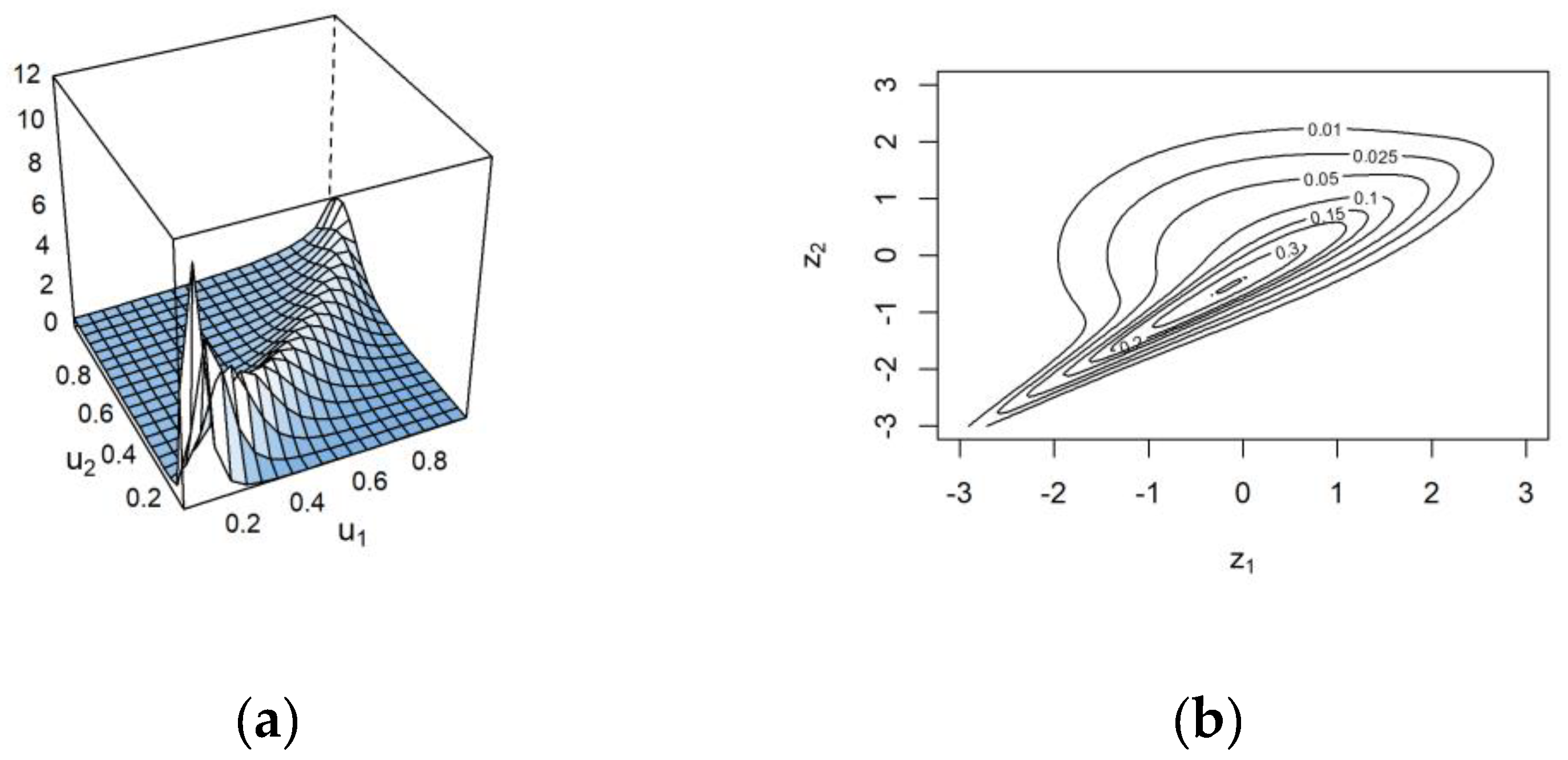
For the intensity and severity relationship,
Table 4 shows that the best model was the 180°-rotated Tawn type 1, according to the log-likelihood, AIC, and BIC values bolded in the table. Compared to the other considered models, the 180°-rotated Tawn type 1 obtained the highest log-likelihood (159.57) value and the lowest AIC (−315.14) and BIC (−307.72) values. In addition, the 180°-rotated Tawn type 1 provided a Kendall’s tau coefficient of 0.49, which was near the empirical Kendall’s tau coefficient of 0.55, as shown in
Figure 7. This result showed that the 180°-rotated Tawn type 1 preserved a strong degree of positive dependency. A surface plot of the 180°-rotated Tawn type 1 copula density and its contour plot with standard normal margins for the intensity and duration relationship are shown in
Figure 9a and 9b, respectively.
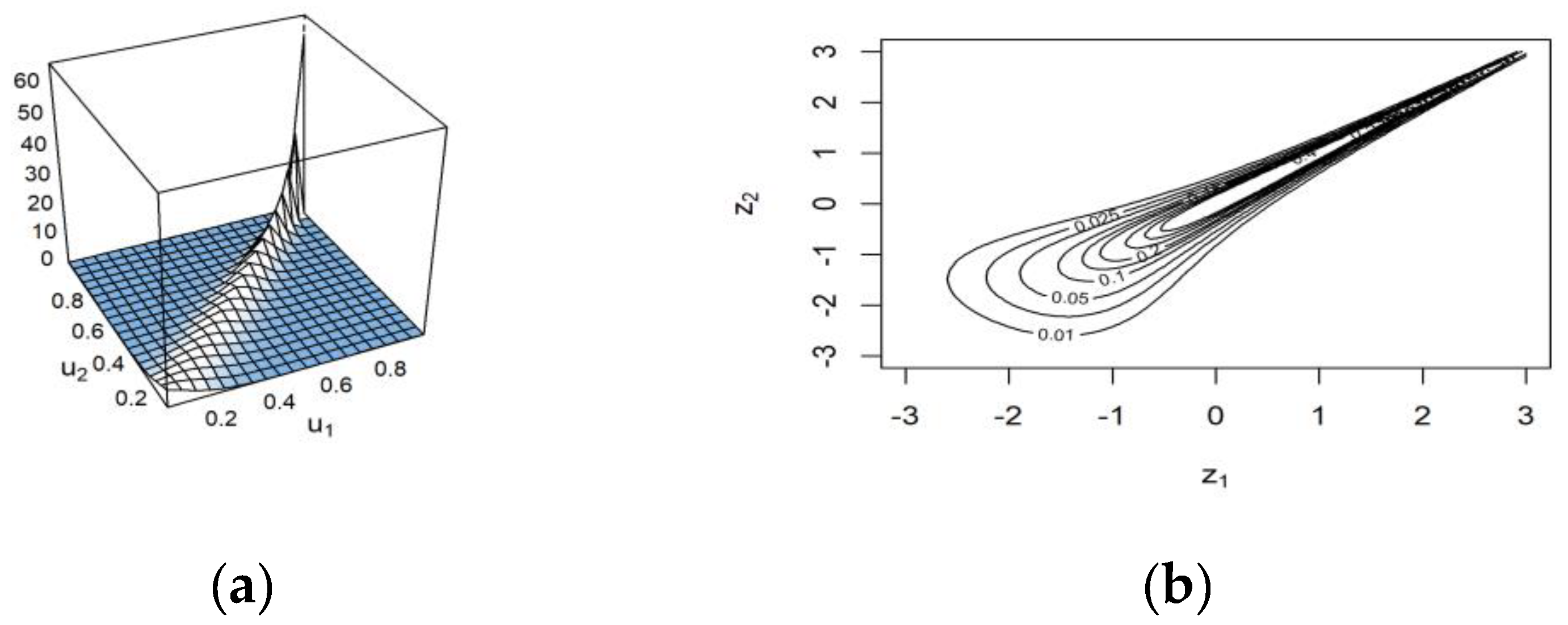
In contrast, for the duration and severity relationship, the obtained log-likelihood, AIC, and BIC values indicated that the Joe was the best bivariate copula model, as shown by the bold font in
Table 5.
Table 5 reported that the Joe had the highest log-likelihood (441.84) value and the lowest AIC (−881.68) and BIC (−877.98) values, indicating that it fit the pair better than other considered models. Moreover, the computed Kendall’s tau coefficient from the Joe was 0.85, which was near the empirical Kendall’s tau coefficient of 0.89, as reported in
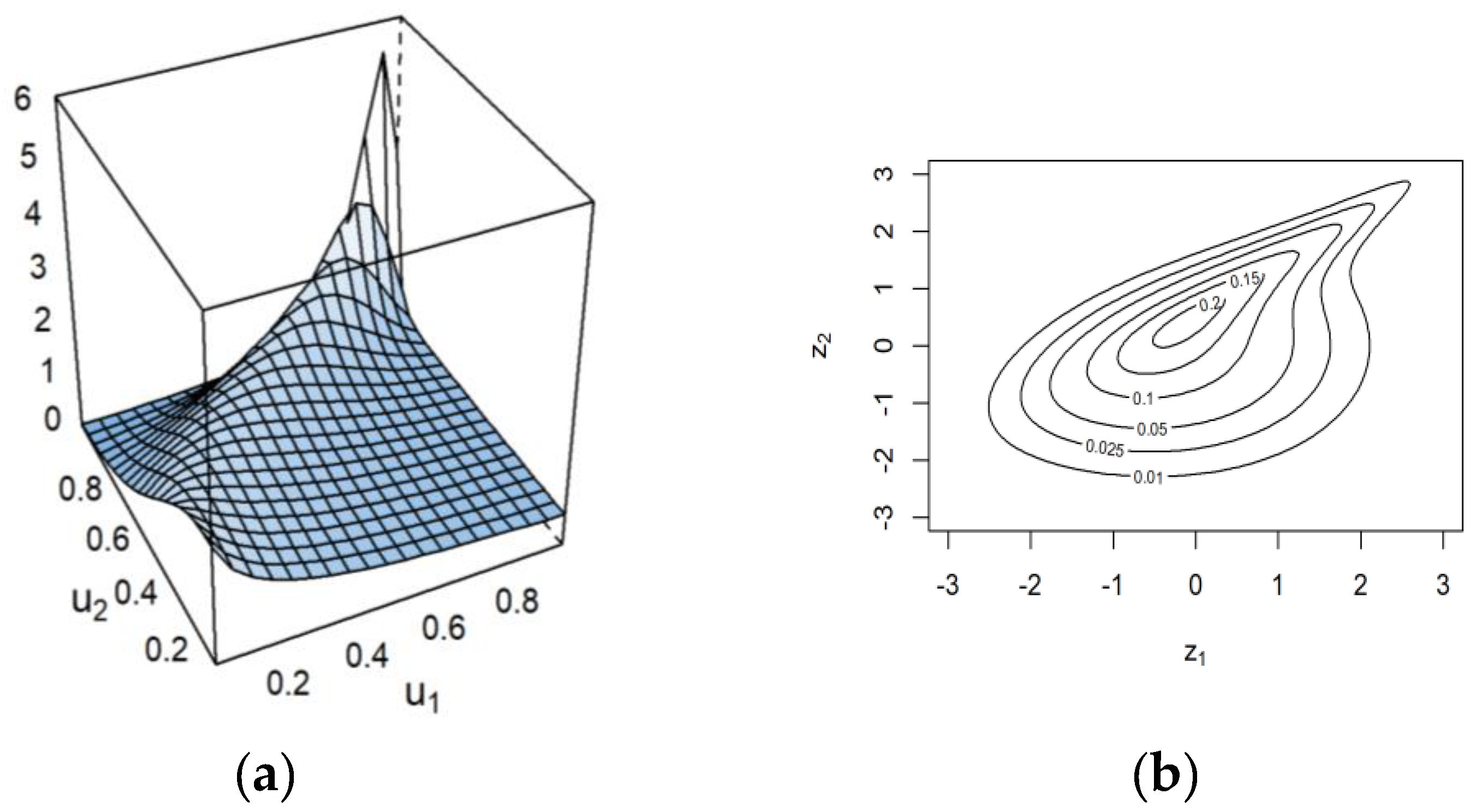
Figure 7. This result showed that the Joe preserved an extremely strong degree of positive dependency. A surface plot of the Joe copula density and its contour plot with standard normal margins for the intensity and duration relationship are shown in
Figure 10a and 10b, respectively.
Table 3.
Parameter estimates, Kendall’s tau, and log-likelihood, AIC, and BIC values for the intensity and duration relationship.
Table 3.
Parameter estimates, Kendall’s tau, and log-likelihood, AIC, and BIC values for the intensity and duration relationship.
| Copula | Par. Num. | Par. 1 | Par. 2 | tau | Log-lik. | AIC | BIC |
|---|
| Gaussian | 1 | 0.59 | 0.00 | 0.40 | 52.57 | −103.15 | −99.44 |
| t | 2 | 0.58 | 30.00 | 0.40 | 52.61 | −101.22 | −93.80 |
| Clayton | 1 | 0.84 | 0.00 | 0.30 | 28.65 | −55.30 | −51.59 |
| Gumbel | 1 | 1.58 | 0.00 | 0.37 | 55.57 | −109.14 | −105.44 |
| Frank | 1 | 3.64 | 0.00 | 0.36 | 44.14 | −86.28 | −82.58 |
| Joe | 1 | 1.83 | 0.00 | 0.31 | 53.85 | −105.69 | −101.98 |
| BB1 | 2 | 0.00 | 1.58 | 0.37 | 55.57 | −107.14 | −99.73 |
| BB6 | 2 | 1.07 | 1.51 | 0.36 | 55.60 | −107.20 | −99.79 |
| BB7 | 2 | 1.74 | 0.31 | 0.36 | 55.40 | −106.81 | −99.40 |
| BB8 | 2 | 2.08 | 0.97 | 0.34 | 56.07 | −108.14 | −100.73 |
| Survival Clayton | 1 | 0.99 | 0.00 | 0.33 | 55.96 | −109.93 | −106.22 |
| Survival Gumbel | 1 | 1.57 | 0.00 | 0.36 | 40.64 | −79.28 | −75.57 |
| Survival Joe | 1 | 1.72 | 0.00 | 0.28 | 24.10 | −46.20 | −42.50 |
| Survival BB1 | 2 | 0.82 | 1.11 | 0.36 | 56.48 | −108.96 | −101.55 |
| Survival BB6 | 2 | 1.00 | 1.57 | 0.36 | 40.62 | −77.24 | −69.83 |
| Survival BB7 | 2 | 1.13 | 0.95 | 0.35 | 56.34 | −108.69 | −101.28 |
| Survival BB8 | 2 | 6.00 | 0.47 | 0.34 | 40.44 | −76.88 | −69.47 |
| Tawn type 1 | 2 | 2.62 | 0.42 | 0.32 | 64.67 | −125.33 | −117.92 |
| 180°-rotated Tawn type 1 | 2 | 1.72 | 0.59 | 0.29 | 31.47 | −58.94 | −51.53 |
| Tawn type 2 | 2 | 1.57 | 0.59 | 0.26 | 40.29 | −76.58 | −69.17 |
| 180°-rotated Tawn type 2 | 2 | 1.76 | 0.59 | 0.30 | 38.75 | −73.51 | −66.09 |
Figure 10.
Surface plot of the Joe copula density (a) and its contour plot with standard normal margins (b) for the severity and duration relationship.
Figure 10.
Surface plot of the Joe copula density (a) and its contour plot with standard normal margins (b) for the severity and duration relationship.
Table 4.
Parameter estimates, Kendall’s tau, and log-likelihood, AIC, and BIC values for the intensity and severity relationship.
Table 4.
Parameter estimates, Kendall’s tau, and log-likelihood, AIC, and BIC values for the intensity and severity relationship.
| Copula | Par. Num. | Par. 1 | Par. 2 | tau | Log-lik. | AIC | BIC |
|---|
| Gaussian | 1 | 0.74 | 0.00 | 0.53 | 116.36 | −230.72 | −227.01 |
| t | 2 | 0.70 | 2.78 | 0.49 | 121.38 | −238.76 | −231.35 |
| Clayton | 1 | 1.90 | 0.00 | 0.49 | 115.69 | −229.39 | −225.68 |
| Gumbel | 1 | 1.96 | 0.00 | 0.49 | 106.31 | −210.63 | −206.92 |
| Frank | 1 | 5.42 | 0.00 | 0.48 | 89.43 | −176.86 | −173.15 |
| Joe | 1 | 2.21 | 0.00 | 0.40 | 83.13 | −164.26 | −160.55 |
| BB1 | 2 | 1.04 | 1.42 | 0.54 | 129.43 | −254.86 | −247.44 |
| BB6 | 2 | 1.00 | 1.96 | 0.49 | 106.30 | −208.59 | −201.18 |
| BB7 | 2 | 1.75 | 1.72 | 0.54 | 135.18 | −266.36 | −258.94 |
| BB8 | 2 | 6.00 | 0.62 | 0.47 | 86.36 | −168.71 | −161.30 |
| Survival Clayton | 1 | 1.42 | 0.00 | 0.41 | 87.69 | −173.39 | −169.68 |
| Survival Gumbel | 1 | 2.13 | 0.00 | 0.53 | 125.54 | −249.08 | −245.37 |
| Survival Joe | 1 | 2.68 | 0.00 | 0.48 | 115.37 | −228.73 | −225.02 |
| Survival BB1 | 2 | 0.27 | 1.90 | 0.54 | 128.01 | −252.03 | −244.61 |
| Survival BB6 | 2 | 1.07 | 2.03 | 0.53 | 125.58 | −247.16 | −239.75 |
| Survival BB7 | 2 | 2.36 | 0.97 | 0.54 | 136.81 | −269.63 | −262.22 |
| Survival BB8 | 2 | 2.68 | 1.00 | 0.48 | 115.37 | −226.73 | −219.32 |
| Tawn type 1 | 2 | 2.11 | 0.75 | 0.43 | 100.61 | −197.23 | −189.81 |
| 180°-rotated Tawn type 1 | 2 | 4.70 | 0.58 | 0.49 | 159.57 | −315.14 | −307.72 |
| Tawn type 2 | 2 | 2.08 | 0.75 | 0.43 | 96.36 | −188.72 | −181.31 |
| 180°-rotated Tawn type 2 | 2 | 2.07 | 0.75 | 0.42 | 104.50 | −204.99 | −197.58 |
In
Figure 10a, the Joe copula density increased sharply when
and
approached 1. This behavior showed that the severity and duration were very highly correlated with each other and highlighted that the possibility for severe air pollution events to continue to occur over a long period was high. This result also highlighted the importance of risk awareness for the prolonged, severe, and unhealthy air pollution events.
Henceforth, two scoring goodness-of-fit tests based on the Vuong and Clarke tests were applied to compare the two models. Using these two tests, the model that fit any pair better than the other considered models was identified. Additionally, these tests indicated the best model according to the total obtained score. The comparison results based on the Vuong and Clarke tests for the pairs of the (
,
), (
,
), and (
,
) are provided in
Table 6,
Table 7, and
Table 8, respectively.
Table 5.
Parameter estimates, Kendall’s tau, and log-likelihood, AIC, and BIC values for the duration and severity relationship.
Table 5.
Parameter estimates, Kendall’s tau, and log-likelihood, AIC, and BIC values for the duration and severity relationship.
| Copula | Par. Num. | Par. 1 | Par. 2 | tau | Log-lik. | AIC | BIC |
|---|
| Gaussian | 1 | 0.93 | 0.00 | 0.76 | 280.62 | −559.25 | −555.54 |
| t | 2 | 0.96 | 2.00 | 0.82 | 331.71 | −659.41 | −652.00 |
| Clayton | 1 | 2.75 | 0.00 | 0.58 | 144.35 | −286.70 | −282.99 |
| Gumbel | 1 | 5.98 | 0.00 | 0.83 | 377.95 | −753.90 | −750.19 |
| Frank | 1 | 22.45 | 0.00 | 0.83 | 353.82 | −705.64 | −701.93 |
| Joe | 1 | 11.81 | 0.00 | 0.85 | 441.84 | −881.68 | −877.98 |
| BB1 | 2 | 0.00 | 5.97 | 0.83 | 377.84 | −751.69 | −744.27 |
| BB6 | 2 | 6.00 | 1.77 | 0.84 | 432.39 | −860.77 | −853.36 |
| BB7 | 2 | 5.00 | 0.12 | 0.68 | 352.76 | −701.51 | −694.10 |
| BB8 | 2 | 6.00 | 1.00 | 0.72 | 382.67 | −761.33 | −753.92 |
| Survival Clayton | 1 | 11.10 | 0.00 | 0.85 | 440.08 | −878.16 | −874.45 |
| Survival Gumbel | 1 | 3.69 | 0.00 | 0.73 | 230.44 | −458.88 | −455.17 |
| Survival Joe | 1 | 3.63 | 0.00 | 0.58 | 144.06 | −286.12 | −282.41 |
| Survival BB1 | 2 | 5.00 | 1.72 | 0.83 | 417.01 | −830.02 | −822.61 |
| Survival BB6 | 2 | 1.00 | 3.68 | 0.73 | 230.38 | −456.75 | −449.34 |
| Survival BB7 | 2 | 1.00 | 6.00 | 0.75 | 396.18 | −788.36 | −780.95 |
| Survival BB8 | 2 | 6.00 | 0.85 | 0.63 | 221.85 | −439.70 | −432.29 |
| Tawn type 1 | 2 | 7.10 | 0.96 | 0.83 | 388.06 | −772.12 | −764.70 |
| 180°-rotated Tawn type 1 | 2 | 3.69 | 0.99 | 0.72 | 229.34 | −454.67 | −447.26 |
| Tawn type 2 | 2 | 6.15 | 0.99 | 0.83 | 378.53 | −753.05 | −745.64 |
| 180°-rotated Tawn type 2 | 2 | 5.83 | 0.93 | 0.78 | 263.57 | −523.14 | −515.73 |
Using a non-nested model comparison based on the Vuong and Clarke tests,
Table 6 shows that the Tawn type 1 was the best model because it obtained the highest total score of 21 on the Vuong and Clarke tests. This result was consistent with the above outcomes for the information-based model comparison (log-likelihood, AIC, and BIC). Furthermore, the total scores of the Tawn type 1 were far better than those of the second- and third-best models, which were the BB8 and Gumbel copulas, respectively. On the Vuong and Clarke tests, the BB8 copula obtained scores of 10 and 18, respectively and the Gumbel copula had scores of nine and 15, respectively. Therefore, these tests also indicated that the Tawn type 1 was much more appropriate for the intensity and duration than the other considered models.
In
Table 7, for the intensity and severity relationship, the 180°-rotated Tawn type 1 was reported as the best model since it obtained the highest total score of 21 for the Vuong and Clarke tests. This outcome was similar to the result obtained from the information-based model comparison (log-likelihood, AIC, and BIC). Focusing on the Vuong test, the result showed that the best model was the 180°-rotated Tawn type 1 (21), followed by Survival BB6 (12) and then Survival BB7 (12). In contrast, for the Clarke test, the 180°-rotated Tawn type 1 (21) was almost equivalent to the second-best model, the Tawn type 2 (19), but significantly different from the third-best model, Survival Gumbel (15). However, these tests indicated that the 180°-rotated Tawn type 1 was more suitable for the intensity and duration than the other considered models.
Finally, for the duration and severity relationship,
Table 8 shows that the Joe and Survival Clayton were equally superior because they obtained total scores of 19 and 20 for the Vuong and Clarke tests, respectively. In addition, BB6 was similar to these two models because it had total scores of 19 and 17 for the Vuong and Clarke tests, respectively. These results acknowledged the similarity between these three copula models because their total scores were quite similar. However, considering the outcome of the information-based model comparison (log-likelihood, AIC, and BIC), the Joe model maintained an advantage in modeling the duration and severity relationship over the other considered models. We noted that a similar finding was reported in Masseran [
22] for the duration and severity relationship.
Table 6.
Details on the Vuong test and Clarke tests for the intensity and duration relationship.
Table 6.
Details on the Vuong test and Clarke tests for the intensity and duration relationship.
| Copula | Vuong Test | Clarke Test |
|---|
| Gaussian | 2 | −6 |
| t | 2 | 6 |
| Clayton | −15 | −15 |
| Gumbel | 9 | 15 |
| Frank | 7 | 8 |
| Joe | 6 | 5 |
| BB1 | 9 | 15 |
| BB6 | 8 | 12 |
| BB7 | 6 | 5 |
| BB8 | 10 | 18 |
| Survival Clayton | 6 | −2 |
| Survival Gumbel | −9 | −9 |
| Survival Joe | −18 | −18 |
| Survival BB1 | 6 | 3 |
| Survival BB6 | −11 | −11 |
| Survival BB7 | 6 | 0 |
| Survival BB8 | 4 | 0 |
| Tawn type 1 | 21 | 21 |
| 180°-rotated Tawn type 1 | −17 | −18 |
| Tawn type 2 | −11 | −13 |
| 180°-rotated Tawn type 2 | 0 | 5 |
Based on the abovementioned results, it is also worth noting the possibility where the result of the information-based model comparison (log-likelihood, AIC, and BIC) is not matched by the result of the non-nested model comparison (the Vuong and Clarke tests). This occurs due to the nature of these two comparisons, where the first analyzes the model performance solely based on a single model criterion, without any comparison to another model. In addition, some very simple formulas connecting the log-likelihood, AIC, and BIC can also be derived and used to improve the mathematical models, such as quantitative structure–activity relationship (qSAR) models for understanding how the structure and activity of random variables relate [
43]. In contrast, the second model performed an early comparison to investigate whether there was significant evidence to distinguish between one model’s specifications and another model’s specifications. Therefore, the different focuses in these two tests led to different outcomes and highlighted the need for careful interpretations.
Overall, based on the comparison results obtained from information-based model comparison using the log-likelihood, AIC, and BIC values and the non-nested model comparison using the Vuong and Clarke tests, our findings indicated that the Tawn type 1, 180°-rotated Tawn type 1, and Joe copulas were the best models to fit the relationship for the pairs of the (, ), (, ), and (, ), respectively. This outcome also highlighted that the dependence structures for the pairs were skewed, asymmetric, and non-Gaussian shapes. The latter characteristics established the used copulas as the appropriate models for such dependence structures. Furthermore, these characteristics also highlighted the importance of developing some statistical tests for the skewed, asymmetric, and non-Gaussian shapes, since most of the statistical tests rely on Gaussian shapes.
Table 7.
Details on the Vuong test and Clarke tests for the intensity and severity relationship.
Table 7.
Details on the Vuong test and Clarke tests for the intensity and severity relationship.
| Copula | Vuong Test | Clarke Test |
|---|
| Gaussian | −9 | −9 |
| T | 9 | 12 |
| Clayton | 5 | −2 |
| Gumbel | −9 | −8 |
| Frank | −1 | 4 |
| Joe | −18 | −16 |
| BB1 | 7 | 9 |
| BB6 | −11 | −10 |
| BB7 | 6 | 4 |
| BB8 | −7 | −5 |
| Survival Clayton | −16 | −15 |
| Survival Gumbel | 9 | 15 |
| Survival Joe | 10 | −1 |
| Survival BB1 | 9 | 15 |
| Survival BB6 | 12 | 10 |
| Survival BB7 | 12 | 7 |
| Survival BB8 | 9 | 4 |
| Tawn type 1 | −17 | −19 |
| 180°-rotated Tawn type 1 | 21 | 21 |
| Tawn type 2 | 9 | 19 |
| 180°-rotated Tawn type 2 | −9 | −14 |
For future studies, these obtained models can be further extended through the vine copula approach to provide a more comprehensive insight into the tri-variate relationship between the duration, intensity, and severity. Furthermore, some recent tests for the general distributions also have been developed. Such tests have been applied to detect the outliers for the continuous distributions based on the cumulative distribution function and to detect the extreme values with order statistics in the samples from the continuous distributions. Therefore, these tests can also be explored further in future research to better understand air pollution behavior.
Table 8.
Details on the Vuong test and Clarke test for the relationship between duration and severity.
Table 8.
Details on the Vuong test and Clarke test for the relationship between duration and severity.
| Copula | Vuong Test | Clarke Test |
|---|
| Gaussian | −5 | −4 |
| t | −1 | 0 |
| Clayton | −18 | −19 |
| Gumbel | 9 | 9 |
| Frank | −1 | 5 |
| Joe | 19 | 20 |
| BB1 | 8 | 6 |
| BB6 | 19 | 17 |
| BB7 | −1 | −4 |
| BB8 | 3 | 0 |
| Survival Clayton | 19 | 20 |
| Survival Gumbel | −10 | −11 |
| Survival Joe | −18 | −17 |
| Survival BB1 | 15 | 15 |
| Survival BB6 | −12 | −13 |
| Survival BB7 | 9 | 4 |
| Survival BB8 | −11 | −15 |
| Tawn type 1 | 10 | 13 |
| 180°-rotated Tawn type 1 | −11 | −8 |
| Tawn type 2 | 9 | 11 |
| 180°-rotated Tawn type 2 | −11 | −8 |
6. Conclusions
This study examined the bivariate dependence structures among the characteristics of unhealthy air pollution events, namely, the duration, severity, and intensity. Air pollution is classified as unhealthy when the API values cross a certain threshold. For Malaysia, the threshold is equal to 100. For each non-overlapping period of an unhealthy air pollution event, the duration is the total number of days of that period, the severity is the summation of all the API values within that period, and the intensity is the maximum API value within that period.
For modeling purposes, copula models were suggested to fit the bivariate dependence structure for all the possible pairs, including the (intensity, duration), (intensity, severity), and (duration, severity). The normalized contour plots of the pairs illustrated that the pairs had skewed, asymmetric, and non-Gaussian shapes. Therefore, the copula models were suitable for this application because they provided a great flexibility in modeling multivariate non-Gaussian distributions due to the separation of the margins and dependence by the copula function.
A wide range of existing parametric copula models were fitted on each pair and optimized using the MLE. Then, the best model was determined based on two comparison methods. The first method was the information-based model comparison that relied on the log-likelihood estimate and the AIC and BIC criteria. The second method was a non-nested model comparison based on the Vuong and Clarke tests.
According to the results of these two comparison methods, the Tawn type 1, 180°-rotated Tawn type 1, and Joe copulas were the best models to fit the relationship for the pairs of the (intensity, duration), (intensity, severity), and (duration, severity), respectively. These models showed that the dependence structures for the pairs were skewed, and the obtained copula models were appropriate tools for such structures. In future work, these obtained models can be further extended through the vine copula approach to provide a more comprehensive insight into the tri-variate relationship of the duration–intensity–severity characteristics.


