
Highly Dispersive Optical Solitons in the Absence of Self-Phase Modulation by Lie Symmetry

 , ,
, , 
 ,
,  , and
, and 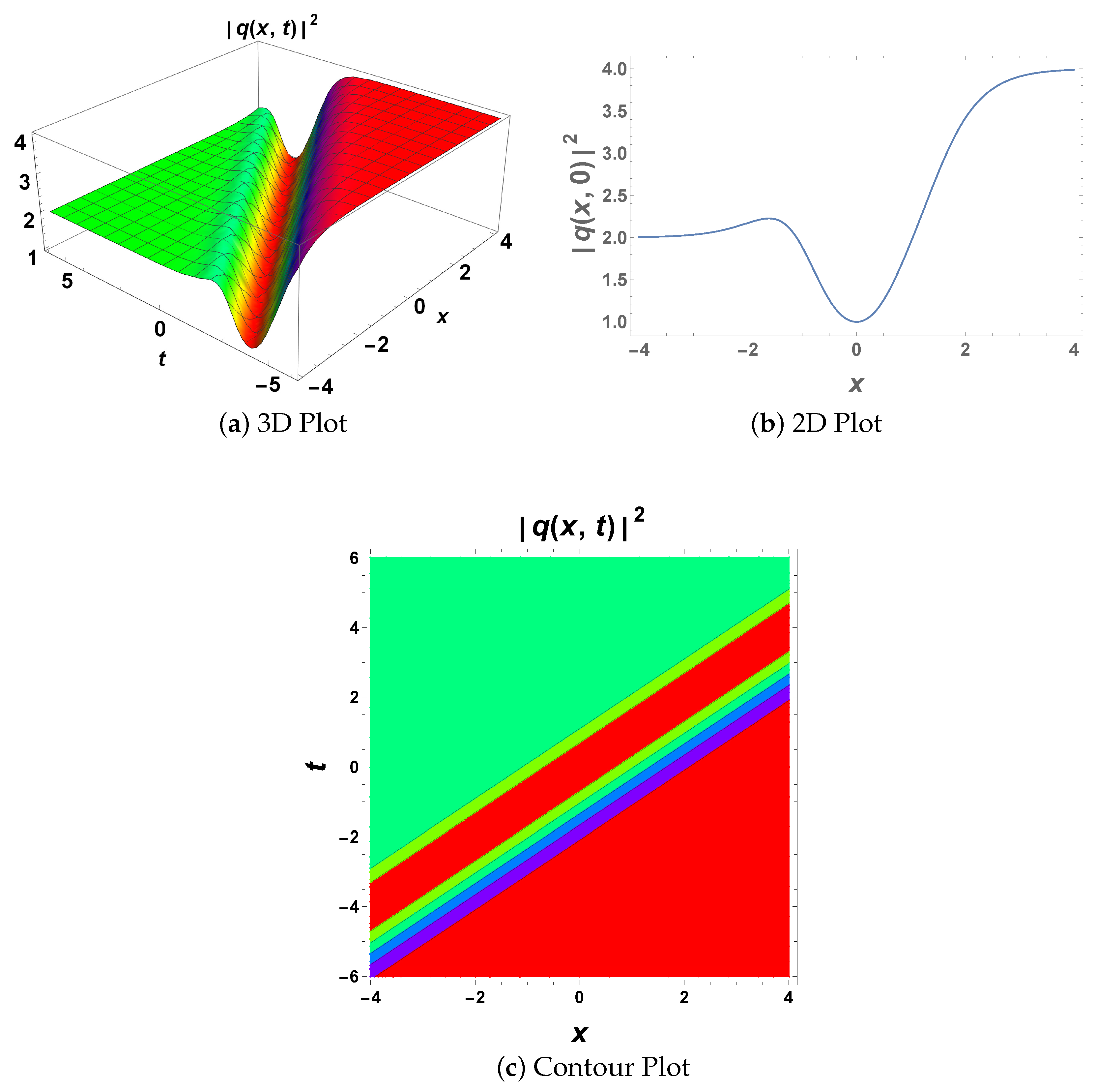
Abstract
1. Introduction
Governing Equation
2. Lie Symmetry Analysis
3. Integration Schemes and Optical Solitons
3.1. Riccati Equation Method
3.2. Improved Modified Extended Tanh-Function Method
4. Conservation Laws
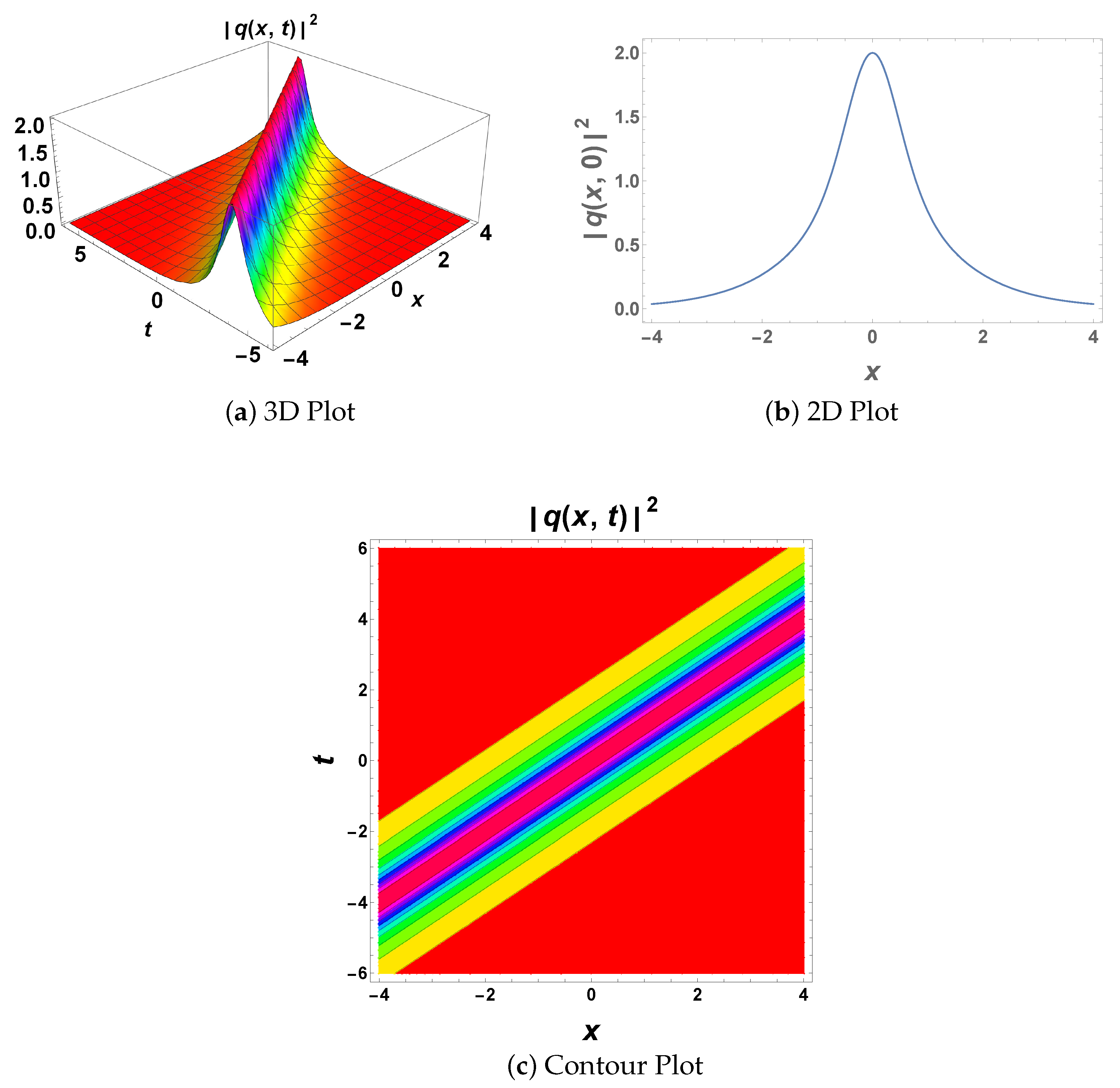
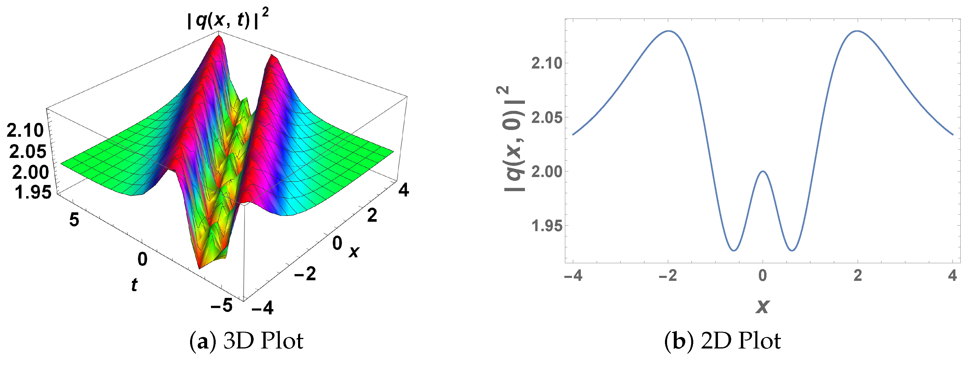
5. Physical Interpretation
6. Conclusions
Author Contributions
Funding
Institutional Review Board Statement
Informed Consent Statement
Data Availability Statement
Acknowledgments
Conflicts of Interest
References
- Biswas, A.; Ekici, M.; Sonmezoglu, A.; Belic, M.R. Highly dispersive optical solitons in absence of self-phase modulation by exp-function. Optik 2019, 186, 436–442. [Google Scholar] [CrossRef]
- González-Gaxiola, O.; Biswas, A.; Moraru, L.; Moldovanu, S. Highly Dispersive Optical Solitons in Absence of Self-Phase Modulation by Laplace-Adomian Decomposition. Photonics 2023, 10, 114. [Google Scholar] [CrossRef]
- Ullah, N.; Rehman, H.U.; Imran, M.; Abdeljawad, T. Highly dispersive optical solitons with cubic law and cubic-quintic-septic law nonlinearities. Results Phys. 2020, 17, 103021. [Google Scholar] [CrossRef]
- Vinita; Ray, S.S. Invariant analysis, optimal system, power series solutions and conservation laws of Kersten-Krasil’shchik coupled KdV-mKdV equations. J. Geom. Phys. 2022, 182, 104677. [Google Scholar] [CrossRef]
- Bluman, G.; Anco, S. Symmetry and Integration Methods for Differential Equations; Springer Science & Business Media: Berlin/Heidelberg, Germany, 2008; Volume 154. [Google Scholar]
- Olver, P.J. Applications of Lie Groups to Differential Equations; Springer Science & Business Media: Berlin/Heidelberg, Germany, 1993; Volume 107. [Google Scholar]
- Kumar, S.; Malik, S.; Biswas, A.; Zhou, Q.; Moraru, L.; Alzahrani, A.; Belic, M. Optical solitons with Kudryashov’s equation by Lie symmetry analysis. Phys. Wave Phenom. 2020, 28, 299–304. [Google Scholar] [CrossRef]
- Yıldırım, Y.; Biswas, A.; Ekici, M.; Triki, H.; Gonzalez-Gaxiola, O.; Alzahrani, A.K.; Belic, M.R. Optical solitons in birefringent fibers for Radhakrishnan–Kundu–Lakshmanan equation with five prolific integration norms. Optik 2020, 208, 164550. [Google Scholar] [CrossRef]
- Malik, S.; Almusawa, H.; Kumar, S.; Wazwaz, A.M.; Osman, M. A (2+1)-dimensional Kadomtsev–Petviashvili equation with competing dispersion effect: Painlevé analysis, dynamical behavior and invariant solutions. Results Phys. 2021, 23, 104043. [Google Scholar] [CrossRef]
- Yang, Z.; Hon, B.Y. An improved modified extended tanh-function method. Z. Naturforschung A 2006, 61, 103–115. [Google Scholar] [CrossRef]
- Arnous, A.H.; Mirzazadeh, M.; Akbulut, A.; Akinyemi, L. Optical solutions and conservation laws of the Chen–Lee–Liu equation with Kudryashov’s refractive index via two integrable techniques. Waves Random Complex Media, 2022; in press. [Google Scholar] [CrossRef]
- Anco, S.C.; Bluman, G. Direct construction method for conservation laws of partial differential equations Part I: Examples of conservation law classifications. Eur. J. Appl. Math. 2002, 13, 545–566. [Google Scholar] [CrossRef]
- Naz, R.; Naeem, I.; Khan, M. Conservation laws of some physical models via symbolic package GeM. Math. Probl. Eng. 2013, 2013, 897912. [Google Scholar] [CrossRef]
- Biswas, A.; Konar, S. Introduction to Non-Kerr Law Optical Solitons; CRC Press: Boca Raton, FL, USA, 2006. [Google Scholar]
- Zhao, Y.H.; Mathanaranjan, T.; Rezazadeh, H.; Akinyemi, L.; Inc, M. New solitary wave solutions and stability analysis for the generalized (3 + 1)-dimensional nonlinear wave equation in liquid with gas bubbles. Results Phys. 2022, 43, 106083. [Google Scholar] [CrossRef]
- Mathanaranjan, T.; Rezazadeh, H.; Şenol, M.; Akinyemi, L. Optical singular and dark solitons to the nonlinear Schrödinger equation in magneto-optic waveguides with anti-cubic nonlinearity. Opt. Quantum Electron. 2021, 53, 722. [Google Scholar] [CrossRef]
- Hirota, R. The Direct Method in Soliton Theory; Number 155; Cambridge University Press: Cambridge, UK, 2004. [Google Scholar]
- Nguyen, L.T.K. Wronskian formulation and Ansatz method for bad Boussinesq equation. Vietnam J. Math. 2016, 44, 449–462. [Google Scholar] [CrossRef]
- Ma, W.X. N-soliton solutions and the Hirota conditions in (2+1)-dimensions. Opt. Quantum Electron. 2020, 52, 511. [Google Scholar] [CrossRef]
- Kudryashov, N.A. Highly dispersive optical solitons of the sixth-order differential equation with arbitrary refractive index. Optik 2022, 259, 168975. [Google Scholar] [CrossRef]
- Kudryashov, N.A. Highly dispersive optical solitons of an equation with arbitrary refractive index. Regul. Chaotic Dyn. 2020, 25, 537–543. [Google Scholar] [CrossRef]
- Kudryashov, N.A. Highly dispersive optical solitons of equation with various polynomial nonlinearity law. Chaos Solitons Fractals 2020, 140, 110202. [Google Scholar] [CrossRef]
- Mathanaranjan, T.; Kumar, D.; Rezazadeh, H.; Akinyemi, L. Optical solitons in metamaterials with third and fourth order dispersions. Opt. Quantum Electron. 2022, 54, 271. [Google Scholar] [CrossRef]
- Kudryashov, N.A. Highly dispersive solitary wave solutions of perturbed nonlinear Schrödinger equations. Appl. Math. Comput. 2020, 371, 124972. [Google Scholar] [CrossRef]
- Fan, E.; Zhang, H. A note on the homogeneous balance method. Phys. Lett. A 1998, 246, 403–406. [Google Scholar] [CrossRef]
- Nguyen, L.T.K. Modified homogeneous balance method: Applications and new solutions. Chaos Solitons Fractals 2015, 73, 148–155. [Google Scholar]
- Arnous, A.H.; Biswas, A.; Kara, A.H.; Yıldırım, Y.; Alshehri, H.M.; Belic, M.R. Highly dispersive optical solitons and conservation laws in absence of self–phase modulation with new Kudryashov’s approach. Phys. Lett. A 2022, 431, 128001. [Google Scholar] [CrossRef]
- Biswas, A.; Ekici, M.; Sonmezoglu, A.; Belic, M.R. Highly dispersive optical solitons in absence of self-phase modulation by Jacobi’s elliptic function expansion. Optik 2019, 189, 109–120. [Google Scholar] [CrossRef]
- Biswas, A.; Ekici, M.; Sonmezoglu, A.; Alshomrani, A.S. Highly dispersive optical solitons in absence of self-phase modulation by F-expansion. Optik 2019, 187, 258–270. [Google Scholar] [CrossRef]
- Hirota, R. Exact Solution of the Korteweg—de Vries Equation for Multiple Collisions of Solitons. Phys. Rev. Lett. 1971, 27, 1192–1194. [Google Scholar] [CrossRef]
- Nguyen, L.T.K. Soliton solution of good Boussinesq equation. Vietnam J. Math. 2016, 44, 375–385. [Google Scholar] [CrossRef]
- Ma, W.X.; You, Y. Solving the Korteweg-de Vries equation by its bilinear form: Wronskian solutions. Trans. Am. Math. Soc. 2005, 357, 1753–1778. [Google Scholar] [CrossRef]
- Neill, D.R.; Atai, J. Gap solitons in a hollow optical fiber in the normal dispersion regime. Phys. Lett. A 2007, 367, 73–82. [Google Scholar] [CrossRef]
- Atai, J.; Malomed, B.A.; Merhasin, I.M. Stability and collisions of gap solitons in a model of a hollow optical fiber. Opt. Commun. 2006, 265, 342–348. [Google Scholar] [CrossRef]
- Chen, Y.; Atai, J. Dark optical bullets in light self-trapping. Opt. Lett. 1995, 20, 133–135. [Google Scholar] [CrossRef]
- Wazwaz, A.M.; Albalawi, W.; El-Tantawy, S. Optical envelope soliton solutions for coupled nonlinear Schrödinger equations applicable to high birefringence fibers. Optik 2022, 255, 168673. [Google Scholar] [CrossRef]
- Wazwaz, A.M.; El-Tantawy, S.A. Optical Gaussons for nonlinear logarithmic Schrödinger equations via the variational iteration method. Optik 2019, 180, 414–418. [Google Scholar] [CrossRef]
- Kaur, L.; Wazwaz, A.M. Bright–dark optical solitons for Schrödinger-Hirota equation with variable coefficients. Optik 2019, 179, 479–484. [Google Scholar] [CrossRef]
- Esen, H.; Secer, A.; Ozisik, M.; Bayram, M. Dark, bright and singular optical solutions of the Kaup–Newell model with two analytical integration schemes. Optik 2022, 261, 169110. [Google Scholar] [CrossRef]
- Ozdemir, N.; Secer, A.; Ozisik, M.; Bayram, M. Perturbation of dispersive optical solitons with Schrödinger–Hirota equation with Kerr law and spatio-temporal dispersion. Optik 2022, 265, 169545. [Google Scholar] [CrossRef]
- Cinar, M.; Secer, A.; Ozisik, M.; Bayram, M. Derivation of optical solitons of dimensionless Fokas-Lenells equation with perturbation term using Sardar sub-equation method. Opt. Quantum Electron. 2022, 54, 402. [Google Scholar] [CrossRef]
- Serkin, V.N.; Belyaeva, T.L. High-energy optical Schrödinger solitons. J. Exp. Theor. Phys. Lett. 2001, 74, 573–577. [Google Scholar] [CrossRef]
- Dianov, E.M.; Nikonova, Z.; Prokhorov, A.M.; Serkin, V.N. Optimal compression of multisoliton pulses in fiber-optic waveguides. Pisma Zhurnal Tekhnischeskoi Fiz. 1986, 12, 756–760. [Google Scholar]
- Afanasyev, V.V.; Vysloukh, V.A.; Serkin, V.N. Decay and interaction of femtosecond optical solitons induced by the Raman self-scattering effect. Opt. Lett. 1990, 15, 489–491. [Google Scholar] [CrossRef]


Disclaimer/Publisher’s Note: The statements, opinions and data contained in all publications are solely those of the individual author(s) and contributor(s) and not of MDPI and/or the editor(s). MDPI and/or the editor(s) disclaim responsibility for any injury to people or property resulting from any ideas, methods, instructions or products referred to in the content. |
© 2023 by the authors. Licensee MDPI, Basel, Switzerland. This article is an open access article distributed under the terms and conditions of the Creative Commons Attribution (CC BY) license (https://creativecommons.org/licenses/by/4.0/).
Share and Cite
Malik, S.; Kumar, S.; Biswas, A.; Yıldırım, Y.; Moraru, L.; Moldovanu, S.; Iticescu, C.; Alotaibi, A. Highly Dispersive Optical Solitons in the Absence of Self-Phase Modulation by Lie Symmetry. Symmetry 2023, 15, 886. https://doi.org/10.3390/sym15040886
Malik S, Kumar S, Biswas A, Yıldırım Y, Moraru L, Moldovanu S, Iticescu C, Alotaibi A. Highly Dispersive Optical Solitons in the Absence of Self-Phase Modulation by Lie Symmetry. Symmetry. 2023; 15(4):886. https://doi.org/10.3390/sym15040886
Chicago/Turabian StyleMalik, Sandeep, Sachin Kumar, Anjan Biswas, Yakup Yıldırım, Luminita Moraru, Simona Moldovanu, Catalina Iticescu, and Abdulaziz Alotaibi. 2023. "Highly Dispersive Optical Solitons in the Absence of Self-Phase Modulation by Lie Symmetry" Symmetry 15, no. 4: 886. https://doi.org/10.3390/sym15040886
APA StyleMalik, S., Kumar, S., Biswas, A., Yıldırım, Y., Moraru, L., Moldovanu, S., Iticescu, C., & Alotaibi, A. (2023). Highly Dispersive Optical Solitons in the Absence of Self-Phase Modulation by Lie Symmetry. Symmetry, 15(4), 886. https://doi.org/10.3390/sym15040886