Article

A Low SNR Signal-Sensing Method Based on a Multiple-Antenna Covariance Matrix

Beijing Research Institute of Telemetry, Beijing 100076, China
*
Author to whom correspondence should be addressed.
Symmetry 2023, 15(4), 888; https://doi.org/10.3390/sym15040888
Submission received: 16 February 2023 / Revised: 27 March 2023 / Accepted: 7 April 2023 / Published: 9 April 2023
(This article belongs to the Special Issue Research on Motor and Special Electromagnetic Device of Symmetry II)

Abstract

:
In this paper, we propose a promising signal-sensing method based on both single- and multiple-antenna covariance matrices of the received signal. In comparison with microwave diagnostics or energy detection, the proposed method does not need prior information of signal and noise. Therefore, it can be widely used in noise power uncertainty scenarios, such as signal transmission in hypersonic plasma sheath, with symmetry to the signal-sensing method in cognitive radio. Designing an efficient signal-sensing method that supports both the application for the field of hypersonic plasma sheath communication or cognitive radio is still an attractive subject deserving of study in symmetry journals. Theoretical analysis and the implementation algorithm of a single-antenna covariance matrix are carried out for the proposed method, with a possible extension to multiple-antenna situations. Simulations show the proposed method has excellent performance, even for very low signal-noise-ratio (SNR) signals, and is competitive with state-of-the-art algorithms.

1. Introduction

When a spacecraft enters the atmosphere at a hypersonic velocity, the air will be ionized at the shock front created by the high-speed vehicle; thus, the surface of the aircraft is enveloped by a hypersonic plasma sheath. The sheath then absorbs, scatters, and reflects microwaves, resulting in a severe decrease in or even a complete loss of the strength of radio-frequency (RF) signals between the reentry vehicle and the ground, which is called a “communications blackout” or simply a “blackout” [1].
A blackout may lead to many problems—especially the attenuation of the signal—that will cause the loss of data telemetry and/or the loss of vehicle control, etc. Moreover, the fluctuation of the electron density will lead to a significant level of signal uncertainty. To evaluate the attenuation of the signal, conventional methods usually use microwave diagnostics, including microwave reflectometry [2,3,4,5], antenna impedance [6,7,8], and/or transmission coefficient [9] diagnostics. These methods are based on reflection and/or transmission coefficients measurements. However, the diagnosed results suffer from inaccuracy when the radio wave frequency is not close to plasma frequency [4]. In addition, these methods usually need prior information about noise, as without such prior information, the diagnosed results are difficult to estimate, especially under a low signal-to-noise ratio (SNR) condition.
To overcome these difficulties, it is necessary to directly investigate sensing (or detecting) methods for low SNR signals. However, few signal-sensing schemes in a hypersonic plasma sheath environment are publicly reported. On the other hand, signal-sensing schemes are widely used in other fields. Based on the symmetry to signal-sensing methods in the cognitive radio field, we can adopt such methods as a reasonable reference. In the cognitive radio field, spectrum/signal-sensing schemes are widely used, such as the energy-detection method [10,11,12,13], the matched-filtering method [14,15], and the cyclostationary-detection method [16,17].
Let us compare these methods. The matched-filtering method requires knowledge of the waveforms and channels of the detected signal, which makes it difficult for practical implementation [18]. The cyclostationary-detection method requires knowledge of cyclic frequencies of the detected signal, with high computational complexity. The energy-detection (ED) method does not need any information about the detected signal and, thus, it is robust with respect to unknown dispersive channels. However, like microwave diagnostics methods, energy detection relies on the knowledge of accurate noise level information. Thus, inaccurate estimation of the noise level leads to an SNR wall and high probability of false alarm [19].
In recent years, blind detection algorithms, which need no information on source signal or noise level, have become an active research area. These methods include eigenvalue-based, wavelet-based, and covariance-based sensing method. Eigenvalue-based methods use the eigenvalues of the sample covariance matrix to detect signals, including the maximum–minimum eigenvalue (MME) detector [20], the energy-to-minimum eigenvalue (EME) detector [21], and the arithmetic-to-geometric-mean (AGM) detector [22]. Wavelet-based methods use wavelet transform to decompose a wide frequency band into elementary building blocks of sub-bands [23,24], which leads to a high computational complexity. Covariance-based methods (CBMs) use various statistics of the sample covariance matrix to detect signals [25,26,27]. Compared with eigenvalue-based methods, the computational complexity of the statistics of the sample covariance matrix is significantly lower than that of the eigenvalues. Thus, designing an efficient covariance-based signal-sensing method is an attractive subject deserving of study in symmetry journals.
This paper focuses on covariance-based methods and proposes a method based on both the single- and multiple-antenna covariance matrices of the signal receiver. Multiple-antenna systems have been widely used to improve the transmission performance of wireless communications. The proposed method can well adapt noise power uncertainty, compared to microwave diagnostics or ED methods. Then, in our simulations, we show that the performance of the proposed method is significantly better than those of the EME or AGM algorithms, and slightly better than those of the MME or CBM algorithms.
The rest of this paper is organized as follows. In Section 2, the system models for single-antenna and multiple-antenna sensing are provided. The theoretical analysis is presented in Section 3. In Section 4, the algorithms for implementation and some simulation results are represented. A comparison of the covariance matrix sensing (CMS) method with the energy detection method is discussed in Section 5. Finally, the paper’s conclusions are provided in Section 6.

2. System Models

2.1. The Single-Antenna Model

Let x ( n ) = s ( n ) + η ( n ) be the received signal at the nth discrete moment, where s(n) is the signal and η(n) is the noise. Note that η(n) is assumed to be a stationary process, satisfying E ( η ( n ) ) = 0 , E ( η 2 ( n ) ) = σ η 2 , and E ( η ( n ) η ( n τ ) ) = 0 for any τ   0 , where E ( . ) denotes the expectation function.
The signal-sensing problem can be formulated as the binary hypothesis test by
H 0 : x ( n ) = η ( n ) , n = 0 , , Ν S 1 H 1 : x ( n ) = s ( n ) + η ( n ) , n = 0 , , Ν S 1
where H0 represents the no-signal case and H1 represents the case with both signal and noise. Ns is the number of signal samples.
Considering L (smoothing factor) consecutive samples and defining:
x(n) = [x(n), x(n − 1), …, x(nL + 1)]T
s(n) = [s(n), s(n − 1), …, s(nL + 1)]T
η(n) = [η(n), η(n − 1), …, η(nL + 1)]T
The statistical covariance matrices of the signal and noise can be defined as:
Rx = E[x(n) xT(n)]
Rs = E[s(n) sT(n)]
Considering that the noise is independently and identically distributed (iid) with a zero mean, we obtain the following:
R x = R s + σ η 2 I L
where IL is the identity matrix of order L. If the received s(n) absents, Rs = 0. Hence, Rx is a diagonal matrix, and the off-diagonal elements of Rx are all zeros. If the received s(n) exists, the signal samples are correlated, and the off-diagonal elements of Rx are non-zero. Thus, in general, one should always obtain certain non-zero off-diagonal elements of Rx.
For signal processing convenience, we usually calculate the statistical covariance matrix by using a limited number of signal samples. Let the number of computed samples be Ns; then, the sample auto-correlations of the received signal can be defined as:
λ ( l ) = 1 N s m = 0 N s 1 x ( m ) x ( m l ) , l = 0 , 1 , , L 1
The statistical covariance matrix Rx can be approximated by the sample covariance matrix, defined as
R x ( N s ) = λ ( 0 ) λ ( 1 ) λ ( L 1 ) λ ( 1 ) λ ( 0 ) λ ( L 2 ) λ ( L 1 ) λ ( L 2 ) λ ( 0 )
where the dimension of R x ( N s ) is L × L.
Without signals, we have
E ( λ ( 0 ) ) = σ η 2
E ( λ ( l ) ) = 0 , l = 0 , 1 , , L 1
With signals, by the signal power σ S 2 = E ( s 2 ( n ) ) and the normalized correlation among the signal samples, we have
α ( l ) = E [ s ( n ) s ( n l ) ] / σ S 2
where 0 α ( l ) 1 , we then have
E ( λ ( 0 ) ) = σ S 2 + σ η 2
E ( λ ( l ) ) = α l σ S 2 , l = 0 , 1 , , L 1
as well as the average sum of all elements of matrix Rx,
T 1 ( N S ) = 1 L l = 1 L λ ( 0 ) + 2 L l = 1 L 1 ( L l ) λ ( l )
and the average sum of diagonal elements of matrix Rx
T 2 ( N S ) = 1 L l = 1 L λ ( 0 )
According to Equations (10)–(14), with no signal, T 1 ( N S ) T 2 ( N S ) = 1 , and with signals, T 1 ( N S ) T 2 ( N S ) > 1 . Hence, the ratio T 1 ( N S ) T 2 ( N S ) can be used to sense the presence of the signal.

2.2. The Multiple-Antenna Model

We first assume that there are M antennae at the receiver (M ≥ 1). The received signal at the nth discrete moment at receiver i, xi(n), is given by
xi(n) = si(n) + ηi(n), i = 1, …, M
where si(n) (ηi(n)) is the signal (noise) at receiver i. Then, the signal-sensing problem can be formulated as
H0: xi(n) = ηi(n), i = 1, , M
H1: xi(n) = si(n) + ηi(n), i = 1, , M
Considering the L consecutive samples and defining the following vectors
xi(n) = [xi(n), xi(n − 1), …, xi(nL + 1)]T
si(n) = [si(n), si(n − 1), …, si(nL + 1)]T
ηi(n) = [ηi(n), ηi(n − 1), …, ηi(nL + 1)]T
and, then, further combining all the signals from the M antennae, we can define the following vectors
X(n) = [x1(n), …, xM(n), x1(n − 1), …, xM(n − 1), …, x1(nL + 1), …, xM(nL + 1)]T
S(n) = [s1(n), …, sM(n), s1(n − 1), …, sM(n − 1), …, s1(nL + 1), …, sM(nL + 1)]T
N(n) = [η1(n), …, ηM(n), η1(n − 1), …, ηM(n − 1), …, η1(nL + 1), …, ηM(nL + 1)]T
The statistical covariance matrices of the signal and noise are written as
RX = E[X(n) X T(n)]
RS = E[S(n) ST(n)]
Again, considering the white noise, we obtain
R X = R S + σ η 2 I M L
where IML is the identity matrix of order ML. Like the antenna situation, if si(n) is absent, RS = 0. Hence, RX is a diagonal matrix and the off-diagonal elements of RX are all zeros. If si(n) is present, the off-diagonal elements of RX are not zeros.
Writing the number of available samples by Ns, one can then define the sample auto-correlation of the received signal as
λ i j ( l ) = 1 N S m = 0 N S 1 x i ( m ) x j ( m l ) , l = 0 , 1 , , L 1 ; i , j = 1   2 , M
The statistical covariance matrix RX can be approximated by the sample covariance matrix defined as
R X ( N s ) = λ 11 ( 0 ) λ 12 ( 0 ) λ 1 M ( 0 ) λ 11 ( L 1 ) λ 12 ( L 1 ) λ 1 M ( L 1 ) λ 21 ( 0 ) λ 22 ( 0 ) λ 2 M ( 0 ) λ 21 ( L 1 ) λ 22 ( L 1 ) λ 2 M ( L 1 ) λ M 1 ( 0 ) λ M 2 ( 0 ) λ M M ( 0 ) λ M 1 ( L 1 ) λ M 2 ( L 1 ) λ M M ( L 1 ) λ M 1 ( L 1 ) λ M 2 ( L 1 ) λ M M ( L 1 ) λ M 1 ( 0 ) λ M 2 ( 0 ) λ M M ( 0 )
The dimension of R X ( N s ) is ML × ML.
Without signals, we have
E ( λ i i ( 0 ) ) = σ η 2 , i = 1 , 2 , , M
E ( λ i j ( l ) ) = 0 , i j , i , j = 1 , 2 , , M , l = 0 , 1 , , L 1
With signals, introducing the ith (i = 1,2, …, M) signal power, σ S i 2 = E ( s i 2 ( n ) ) , we have
E ( λ i i ( 0 ) ) = σ S i 2 + σ η 2 , i = 1 , 2 , , M
E ( λ i j ( l ) ) 0 , i j , i , j = 1 , 2 , M ; l = 0 , 1 , , L 1
Then, we further write T 3 ( N S ) as the average sum of all elements of matrix R X ( N s ) and T 4 ( N S ) as the average sum of the diagonal elements of matrix R X ( N s ) . For simplicity, with r n m the element of matrix R X ( N s ) at the nth row and mth column, we have
T 3 ( N S ) = 1 M L n = 1 M L m = 1 M L r n m
T 4 ( N S ) = 1 M L n = 1 M L r n m
According to Equations (29)–(33), without signals, T 3 ( N S ) T 4 ( N S ) = 1 and with signals, T 3 ( N S ) T 4 ( N S ) > 1 . Hence, the single-antenna algorithm can be directly applied for the multiple-antenna case.

2.3. The Computational Complexity

The major complexity of the CMS algorithm comes from two functions: the computation of the covariance matrix (Equation (9) or Equation (29)) and the judgment function of T 1 N S T 2 N S or T 3 N S T 4 N S (Equations (15) and (16) or Equations (34) and (35)). For the first function, the covariance matrix is a block Toeplitz matrix and Hermitian, so that we only need to evaluate its first block row. Hence, M2LNs multiplications and M2L(ns − 1) additions are needed, at most. For the second function, (M2L2 + ML) additions are needed. In general, the total complexity of the multiplications are nearly M2LNs.
For comparison, the ED algorithm requires MNs multiplications and M(ns − 1) additions, which means that the complexity of the CMS algorithm is about ML times higher than that of the ED algorithm. Meanwhile, the total complexity of the MME and EME algorithms are M2LNs + O(M3L3). Therefore, the complexity of the CMS algorithm is less than those of the MME and EME algorithms.

3. Theoretical Analysis

Considering that the single-antenna algorithm can be directly used for the multiple-antenna case, we focus our theoretical analysis on the single-antenna case.
The performance of the signal-sensing algorithm could be described by the probability of detection (Pd) and a false alarm (Pfa). In the ideal case, Pd goes to unity and Pfa goes to zero. With no signal information at the receiver side, we usually choose the threshold based on Pfa. After setting the threshold, we can calculate the Pd at various SNR.
In this section, we analyze the distribution of a random variable and provide theoretical estimations for Pd and Pfa. To achieve this goal, the first task is to find the statistical distribution of T 1 ( N S ) / T 2 ( N S ) .
According to Equations (13)–(16), we have
T 1 ( N S ) = 1 L l = 1 L λ ( 0 ) + 2 L l = 1 L 1 ( L l ) λ ( l )
T 2 ( N S ) = 1 L l = 1 L λ ( 0 )
Based on the central limit theorem, without signals,
E ( λ ( l ) ) = 2 π N S σ η 2 , l = 1 , 2 , , L 1
and with signals, for large Ns and a low SNR situation,
E ( λ ( l ) ) = 2 π N S σ S 2 + σ η 2 2 e τ l 2 2 + E λ l 1 2 π τ l + e u 2 2 d u , l = 1 , 2 , , L 1
From Equations (10)–(14), we have, without signals,
E T 1 N S = 1 + L 1 2 π N S σ η 2
E T 2 N S = σ η 2
and with signals and for the large Ns, we have
E T 1 N S = σ S 2 + σ η 2 + 2 σ S 2 L l = 1 L 1 L l α l 1 2 π τ l + e u 2 2 d u + 2 σ S 2 + σ η 2 L l = 1 L 1 L l 2 π N S 2 e τ l 2 2
E T 2 N S = σ S 2 + σ η 2
Based on these relationships, we find the statistical distribution
T 1 ( N S ) T 2 ( N S ) E T 1 N S E T 2 N S
without signals,
E T 1 N S E T 2 N S = 1 + L 1 2 π N S
and with signals,
E T 1 N S E T 2 N S 1 + σ S 2 σ S 2 + σ η 2 2 L l = 1 L 1 L l α l = 1 + S N R S N R + 1 γ L
where S N R = σ S 2 σ η 2 , γ L = 2 L l = 1 L 1 L l α l
Then, we have
P f a = P T 1 ( N s ) > γ 1 T 2 ( N s ) = P T 2 ( N s ) < 1 γ 1 T 1 ( N s ) = P T 2 ( N s ) < 1 γ 1 1 + ( L 1 ) 2 N s π σ η 2 1 Q 1 γ 1 1 + ( L 1 ) 2 N s π 1 2 N s
where
Q ( t ) = 1 2 π t + e u 2 2 d u
For a given P f a , the threshold is chosen as
1 γ 1 1 + ( L 1 ) 2 N s π 1 2 N s = Q 1 ( P f a )
Then, we have
γ 1 = 1 + ( L 1 ) 2 N s π 1 Q 1 ( P f a ) 2 N s
After setting the threshold, we can obtain the probability of sensing at various SNRs. For a fixed threshold, with the signal,
P d = P T 1 ( N s ) > γ 1 T 2 ( N s ) = P T 2 ( N s ) < 1 γ 1 T 1 ( N s ) P T 2 ( N s ) < 1 γ 1 E ( T 1 ( N s ) ) = P T 2 ( N s ) σ s 2 σ η 2 V a r ( T 2 ( N s ) ) < 1 γ 1 E ( T 1 ( N s ) σ s 2 σ η 2 V a r ( T 2 ( N s ) ) = 1 Q 1 γ 1 E ( T 1 ( N s ) σ s 2 σ η 2 V a r ( T 2 ( N s ) )
For very large Ns and a very low SNR [26],
V a r ( T 2 ( N s ) 2 σ η 2 N s ( 2 σ s 2 + σ η 2 ) 2 ( σ s 2 + σ η 2 ) N s
E ( T 1 ( N s ) σ s 2 + σ η 2 + γ L σ s 2
Hence, we approximately have
P d = 1 Q 1 γ 1 + γ L σ s 2 γ 1 ( σ s 2 + σ η 2 ) 1 2 N s = 1 Q 1 γ 1 + γ L S N R γ 1 ( S N R + 1 ) 1 2 N s
Then, in Equation (54), it is seen that Pd increases with Ns, SNR, and the correlation strength among the signal samples. For a fixed SNR, Pd goes to unity when Ns goes to infinite.

4. Algorithms and Simulations

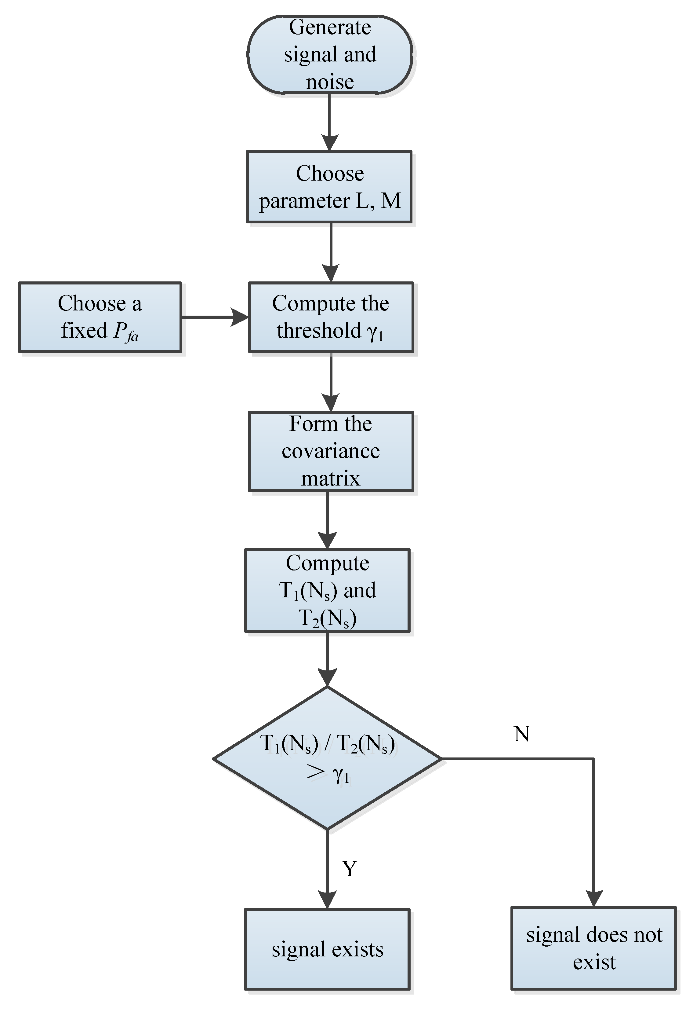
Based on the theoretical analysis, we propose the following CMS algorithm. The algorithm can be used both for the single-antenna case and the multiple-antenna case.
As shown in Figure 1, the CMS algorithm can be implemented by the following steps:
(1)
Step 1
Generate a sample signal and noise with the number of samples Ns. The signal is varied with SNR, and the noise is as random numbers subject to the standard normal distribution.
(2)
Step 2
Choose a smoothing factor L, with the number of antennae M, and M = 1 for the single-antenna model.
(3)
Step 3
With a fixed Pfa, compute the threshold γ 1 .
(4)
Step 4
Compute the auto-correlations of the received signal λ ( l ) , and use Equation (9) or Equation (29) to form the covariance matrix.
(5)
Step 5
Compute the variables of T 1 ( N s ) , T 2 ( N s ) (or T 3 ( N s ) , T 4 ( N s ) for multiple antennae).
(6)
Step 6
Based on T 1 ( N s ) , T 2 ( N s ) and the threshold γ 1 , determine the presence of the signal, i.e., if T 1 ( N s ) / T 2 ( N s ) > γ 1 , the signal exists; otherwise, the signal does not exist. The multiple-antenna cases are similar.
According to the CMS algorithm, we provide certain simulation results for six situations: (1) the receiver-operating characteristics (ROC) curve, (2) Pd curves under different SNRs, (3) Pd curves under different Ns, (4) Pd curves under different L, (5) Pd curves under different M, and (6) a performance comparison with state-of-the-art algorithms. In these simulation runs, the source signal is BPSK modulated, with Rb = 1000 bit/s, and a sampling rate fs = 1 MHz. All simulation results are based on MATLAB, while Monte Carlo simulations are used to obtain an average statistical characteristic. To find out the performance of the algorithm, we compare the CMS to the traditional ED. Although the ED algorithm does not require any information about the signal, to guarantee a reliable detection, the threshold of the ED must be set according to the noise power. Nevertheless, there is always noise uncertainty, usually 1–2 dB in practice [14]. The following simulations consider this situation.
(1)
ROC curve
The ROC curve is a graphic depiction of the relationship between the true and false positive ratios to quantify the tradeoffs of test sensitivity and specificity. We set simulation parameters as follows: the number of samples Ns = 10,000, the smoothing factor L = 8, the signal-to-noise ratio (SNR) = −15 dB or −18 dB, and the number of Monte Carlo (MC) = 5000.
Figure 2 shows the simulation results for the above cases, where the “ED−xdB” indicates the ED algorithm with x−dB noise uncertainty.
As shown in the figure, at a fixed Pfa, the Pd of the CMS is higher than that of ED, showing a better performance of CMS than that of ED.
(2)
Pd curves under different SNRs
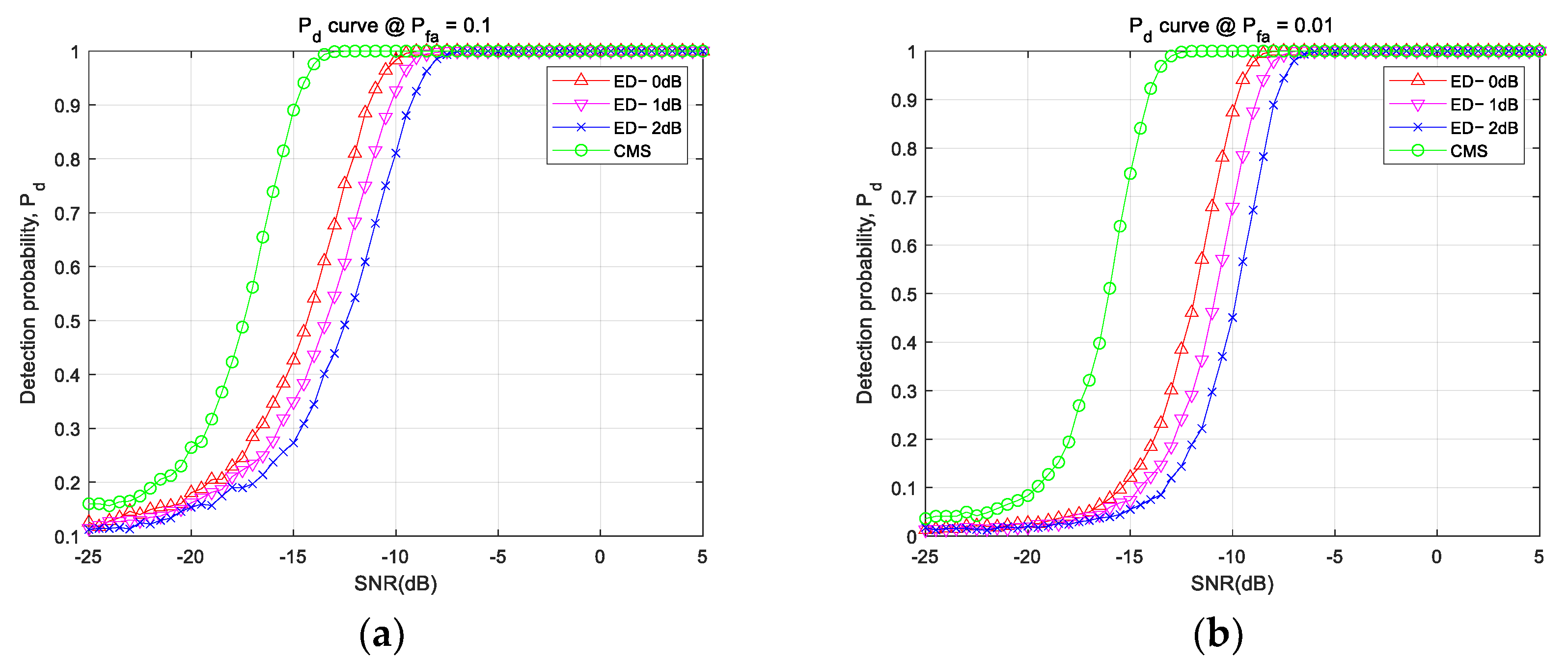
The Pd curves under different SNRs can directly show the performance of the algorithm. Simulation parameters are set as follows: the false alarm Pfa = 0.1 and Pfa = 0.01, the number of samples Ns = 10,000, the smoothing factor L = 8, and the number of Monte Carlo (MC) = 5000. Figure 3 shows the simulation results.
As shown in the figure, the Pd goes to unity for SNR = −13 dB in the case of Ns = 10,000. All Pd curves of ED algorithms go to unity when SNR > −9 dB.
Meanwhile, we noticed that if there is noise uncertainty, the Pd performance of the ED algorithm declines as the uncertainty increases.
(3)
Pd curves under different Ns
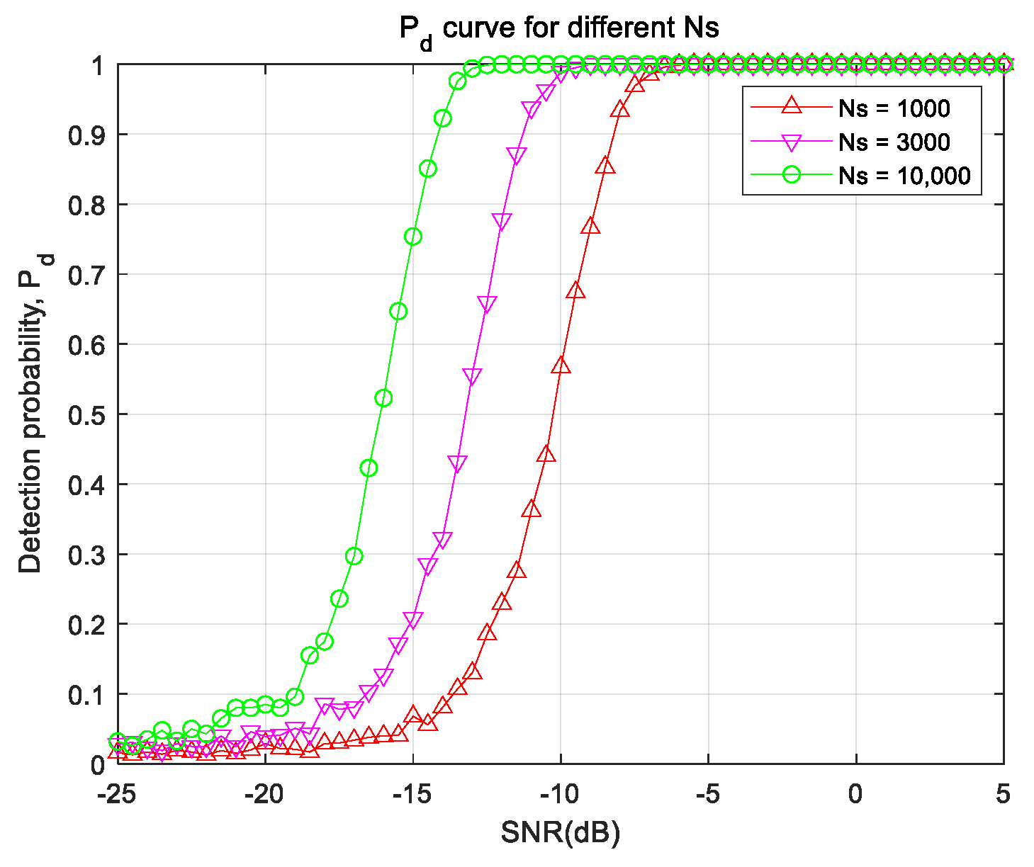
As we know, the performance of the algorithm is closely related to the sensing time. For sample signals, the sensing time is represented by the number of samples Ns. Here, we simulate the Pd curves under different Ns, with simulation parameters set as follows: the false alarm Pfa = 0.01, the number of samples Ns = 1000, Ns = 3000 and Ns = 10,000, the smoothing factor L = 8, and the number of Monte Carlo (MC) = 2000. The simulation result of the CMS algorithm for this case is shown in Figure 4.
From Figure 4, we can see that the Pd goes to unity for SNR = −7 dB in the case of Ns = 1000, and also for SNR = -13dB in the case of Ns = 10,000. It is clear that as Ns gets larger, the Pd performance of the CMS algorithm improves.
(4)
Pd curves under different L
Here, we simulate the influence of smoothing factor L on Pd. Simulation parameters are set as follows: the false alarm Pfa = 0.01, the number of samples Ns = 10,000, the smoothing factor L = 2, L = 4, L = 8, L = 12, L = 16, and the number of Monte Carlo (MC) = 2000. The simulation result of the CMS algorithm for this case is shown in Figure 5.
From Figure 5, we can see that as L becomes larger, the Pd performance of the CMS improves. For example, from L = 4 to 8, we get 2 dB performance improvement. However, the improvement of Pd tends to saturate with the further increase in L. Specifically, from L = 8 to 12, or L = 12 to 16, we obtain only 0.5dB performance improvement, respectively. Therefore, considering larger L means higher complexity, we can choose a proper L according to performance requirements.
(5)
Pd curves for the multiple-antenna situation
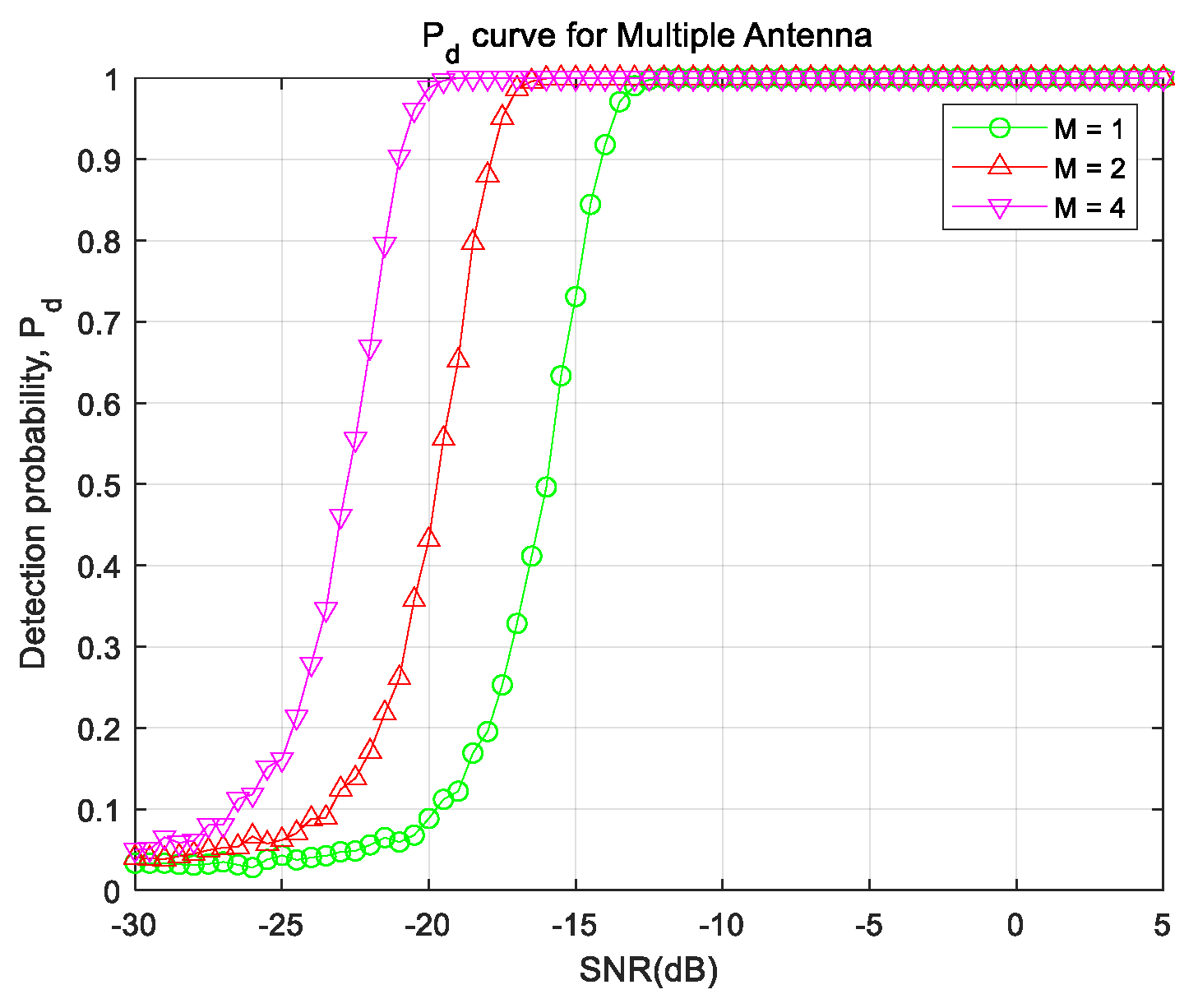
To test multiple-antenna situation, we simulate the performance of the CMS algorithm under different numbers of antennae. For simplicity, assume that the antennae are well separated so that their channels are independent, and that the noise power in each channel is equal. We consider a system with the antenna number M = 1, 2, and 4. Simulation parameters are set as follows: the false alarm Pfa = 0.01, the number of samples Ns = 10,000, the smoothing factor L = 8, and the number of Monte Carlo (MC) = 2000. The simulation result for the CMS algorithm in this case is shown in Figure 6.
From Figure 6, we can see that the larger M is, the more significantly the Pd performance of the CMS is improved. In particular, as the number of antennae doubles, the Pd performance improves about 3 dB.
(6)
Performance comparison with state-of-the-art algorithms
To evaluate the performance of the CMS algorithm, we simulate the performance of the CMS algorithm to compare with some of the state-of-the-art algorithms, including the MME, the EME, the AGM, and the CBM. Simulation parameters are set as follows: the false alarm Pfa = 0.01, the number of samples Ns = 10,000, the smoothing factor L = 8, and the number of Monte Carlo (MC) = 2000. The simulation result for the CMS algorithm in this case is shown in Figure 7.
From Figure 7, we can see that the performance of CMS algorithm is significantly better than those of the AGM and EME algorithms. Meanwhile, the performance of the CMS algorithm is slightly better than those of the MME and CBM algorithms.

5. Discussion

The signal-sensing method is a focused topic in the cognitive radio field, and it is also promoted and applied in other fields, such as signal transmission in a hypersonic plasma sheath. Such a sheath may absorb, scatter, and reflect microwaves, causing significant signal attenuation and noise uncertainty. Traditional microwave diagnostics or energy detection methods require pre-calibrated noise levels, which might be a difficult task on the side of a spacecraft. The proposed CMS method, however, does not need prior information about signals and noise, a feature with great potential for applications.
From the simulation results in Figure 2 and Figure 3, it can be observed that the performance of CMS method is about 5dB better than that of the ideal ED method (without noise uncertainty). Meanwhile, with 1–2dB noise uncertainty, the performance of the ED method might decline as uncertainty increases. Clearly, the CMS method is more advantageous than the ED method.
In addition, from the simulation results in Figure 4 and Figure 5, we can see that the performance of CMS method is closely related to the number of samples Ns and the smoothing factor L. As Ns rises, one obtains more information about the signal and, thus, the Pd performance is improved. Interestingly, a larger L may lead to better performance, but as L becomes larger than 8, the performance improvement becomes less and less. It should also be noted that since a larger L means higher complexity, in practice we can choose an appropriate L, such as L = 8.
Moreover, according to the simulation results in Figure 6, the Pd performance of the CMS algorithm is improved significantly as M increases. This result can be explained by the following two reasons. On the one hand, in the multiple-antenna system, receiving channels are usually independent of each other, so the noises are also independent and their cross-correlations almost vanish. On the other hand, the received signals are related to each other, and the cross-correlation of the signal is considerably finite, so the sensing performance can be improved effectively.
Finally, according to the simulation results in Figure 7, the performance of the CMS algorithm is significantly better than those of the AGM and EME algorithms, and slightly better than those of the MME or CBM algorithms. Thus, it can be demonstrated that the performance of the CMS algorithm is competitive when compared with state-of-the-art algorithms.
6. Conclusions

In this paper, we proposed a promising sensing method based on both the single- and multiple-antenna covariance matrices of the received signal. Theoretical analysis and the implementation algorithm of the single-antenna covariance matrix sensing were provided for the proposed method and extended to multiple-antenna situations. This method can be widely used for various signal-sensing applications, especially scenarios without prior information about signals and noise. Compared with the ED sensing method, the proposed method can effectively overcome the uncertainty of noise. Simulations showed that the proposed method has excellent performance for very low SNR signal and that it is competitive with the state-of-the-art algorithms, such as the AGM, the EME, the MME, or the CBM algorithms. Furthermore, when the received signals are from multiple antennae, the signal cross-correlations improved the sensing performance, which makes the proposed method very promising in mitigating the blackout effect of the hypersonic plasma sheath.

Author Contributions

Conceptualization, Y.Z.; methodology, Y.Z.; software, Y.Z.; validation, Y.Z.; formal analysis, Y.Z. and Y.L.; investigation, Y.Z.; resources, Y.Z.; data curation, Y.Z.; writing—original draft preparation, Y.Z.; writing—review and editing, Y.Z. and Y.L.; visualization, Y.Z.; supervision, Y.L.; project administration, Y.L.; funding acquisition, Y.Z. All authors have read and agreed to the published version of the manuscript.

Funding

This work was supported by the National Natural Science Foundation of China (Grant No. 92271202).

Data Availability Statement

Not applicable.

Conflicts of Interest

The authors declare no conflict of interest.

References

  1. Rybak, J.P.; Churchill, R.J. Progress in Reentry Communications. IEEE Trans. Aerosp. Electron. Syst. AES 1971, 7, 879–894. [Google Scholar] [CrossRef]
  2. Yao, B.; Li, X.; Shi, L.; Liu, Y.; Lei, F.; Zhu, C. Plasma sheath: An equivalent nonlinear mirror between electron density and transmitted electromagnetic signal. Phys. Plasmas 2017, 24, 102–104. [Google Scholar] [CrossRef]
  3. Cataldo, A.; De Benedetto, E. Broadband reflectometry for diagnostics and monitoring applications. IEEE Sens. J. 2010, 11, 451–459. [Google Scholar] [CrossRef]
  4. Yang, M.; Dong, P.; Xie, K.; Li, X.; Quan, L.; Li, J. Broadband microwave reflectometry plasma diagnostic based on invariant point of reflection data. Phys. Plasmas 2021, 28, 102105. [Google Scholar] [CrossRef]
  5. Minashin, P.V.; Kukushkin, A.B. Spectral Intensity of Electron Cyclotron Radiation Emerging from the Plasma to the First Wall in ITER. Symmetry 2023, 15, 118. [Google Scholar] [CrossRef]
  6. Mayhan, J.W.; Caldecott, R.; Bohley, P. Antenna impedance in a reentry environment. IEEE Trans. Antennas Propag. 1968, 16, 573–577. [Google Scholar] [CrossRef]
  7. Swenson, C.M.; Baker, K.D.; Pound, E.; Jensen, M.D. Plasma Diagnostics by Antenna Impedance Measurements. In Lunar and Planetary Inst., Workshop on Advanced Technologies for Planetary Instruments, Part 1; Lunar and Planetary Institute: Houston, TX, USA, 1993; p. 24. [Google Scholar]
  8. Sharma, M.; Vashist, P.C.; Alsukayti, I.; Goyal, N.; Anand, D.; Mosavi, A.H. A Wider Impedance Bandwidth Dual Filter Symmetrical MIMO Antenna for High-Speed Wideband Wireless Applications. Symmetry 2022, 14, 29. [Google Scholar] [CrossRef]
  9. Yang, M.; Li, X.; Bai, B.; Li, Z.; Xue, B. Transmission coefficient estimation based on antenna voltage standing wave ratio under plasma sheath. AIP Adv. 2018, 8, 075018. [Google Scholar] [CrossRef] [Green Version]
  10. Urkowitz, H. Energy detection of unkown deterministic signals. Proc. IEEE 1967, 55, 523–531. [Google Scholar] [CrossRef]
  11. Kay, S.M. Fundamentals of Statistical Signal Processing: Detection Theory; Prentice Hall: Hoboken, NJ, USA, 1998; Volume 2. [Google Scholar]
  12. Kostylev, V.I. Energy detection of a signal with random amplitude. In Proceedings of the Energy Detection of a Signal with Random Amplitude, New York, NY, USA, 28 April–2 May 2002; Volume 3, pp. 1606–1610. [Google Scholar]
  13. Digham, F.F.; Alouini, M.S.; Simon, M.K. On the energy detection of unknown signals over fading channels. IEEE Trans. Commun. 2007, 55, 21–24. [Google Scholar] [CrossRef]
  14. Sahai, A.; Cabric, D. Spectrum sensing: Fundamental limits and practical challenges. In Proceedings of the IEEE International Symposium on New Frontiers DySPAN (Tutorial), Baltimore, MD, USA, 8–11 November 2005. [Google Scholar]
  15. Chen, H.S.; Gao, W.; Daut, D.G. Signature based spectrum sensing algorithms for IEEE 802.22 WRAN. In Proceedings of the 2007 IEEE International Conference on Communications, Glasgow, UK, 24–28 June 2007; pp. 6487–6492. [Google Scholar]
  16. Gardner, W.A. Exploitation of spectral redundancy in cyclostationary signals. IEEE Signal Process. Mag. 1991, 8, 14–36. [Google Scholar] [CrossRef]
  17. Sutton, P.D.; Nolan, K.E.; Doyle, L.E. Cyclostationary signatures in practical cognitive radio applications. IEEE J. Sel. Areas Commun. 2008, 26, 13–24. [Google Scholar] [CrossRef] [Green Version]
  18. Cabric, D.; Mishra, S.M.; Brodersen, R.W. Implementation issues in spectrum sensing for cognitive radios. In Proceedings of the Conference Record of the Thirty-Eighth Asilomar Conference on Signals, Systems and Computers, Pacific Grove, CA, USA, 7–11 November 2004; pp. 772–776. [Google Scholar]
  19. Tandra, R.; Sahai, A. Fundamental limits on detection in low SNR under noise uncertainty. In Proceedings of the 2005 International Conference on Wireless Networks, Communications and Mobile Computing, Maui, HI, USA, 13–16 June 2005. [Google Scholar]
  20. Zeng, Y.; Liang, Y.C. Maximum-minimum eigenvalue detection for cognitive radio. In Proceedings of the 2007 IEEE 18th International Symposium on Personal, Indoor and Mobile Radio Communications, PIMRC’07, Athens, Greece, 3–7 September 2007; pp. 1–5. [Google Scholar]
  21. Zeng, Y.; Liang, Y.-C. Eigenvalue-based spectrum sensing algorithms for cognitive radio. IEEE Trans. Commun. 2009, 57, 1784–1793. [Google Scholar] [CrossRef] [Green Version]
  22. Zeng, Y.; Liang, Y.-C. Robust spectrum sensing in cognitive radio. In Proceedings of the 2010 IEEE 21st International Symposium on Personal, Indoor and Mobile Radio Communications Workshops, Istanbul, Turkey, 26–29 September 2010; pp. 1–8. [Google Scholar]
  23. Tian, Z.; Giannakis, G.B. A wavelet approach to wideband spectrum sensing for cognitive radios. In Proceedings of the 1st International Conference on Cognitive Radio Oriented Wireless Networks and Communications (CROWNCOM ’07), Mykonos, Greece, 8–10 June 2007. [Google Scholar]
  24. Zhang, S.; Wang, Y.; Yuan, H.; Wan, P.; Zhang, Y. Multiple-Antenna Cooperative Spectrum Sensing Based on the Wavelet Transform and Gaussian Mixture Model. Sensors 2019, 19, 3863. [Google Scholar] [CrossRef] [PubMed] [Green Version]
  25. Zeng, Y.H.; Liang, Y.-C. Covariance based signal detections for cognitive radio. In Proceedings of the 2nd IEEE International Symposium on New Frontiers in Dynamic Spectrum Access Networks (DySPAN ’07), Dublin, Ireland, 17–20 April 2007; pp. 202–207. [Google Scholar]
  26. Maida, M.; Najim, J.; Bianchi, P.; Debbah, M. Performance analysis of some eigen-based hypothesis tests for collaborative sensing. In Proceedings of the IEEE Workshop on Statistical Signal Processing, Cardiff, UK, 31 August–3 September 2009. [Google Scholar]
  27. Zeng, Y.H.; Liang, Y.-C. Spectrum-sensing algorithms for cognitive radio based on statistical covariances. IEEE Trans. Veh. Technol. 2009, 58, 1804–1815. [Google Scholar] [CrossRef]
Figure 1. Flow chart for CMS algorithm.
Symmetry 15 00888 g001
Figure 2. ROC curves for CMS and ED algorithms with (a) SNR = −15 dB, and (b) SNR = −18 dB.
Symmetry 15 00888 g002
Figure 3. Pd curves for CMS and ED algorithms with (a) Pfa = 0.1 and (b) Pfa = 0.01.
Symmetry 15 00888 g003
Figure 4. Pd curves for different Ns of CMS.
Symmetry 15 00888 g004
Figure 5. Pd curves for the CMS with different L.
Symmetry 15 00888 g005
Figure 6. Pd curves for the CMS with multiple antennae.
Symmetry 15 00888 g006
Figure 7. Comparison of Pd curves for the different algorithms.
Symmetry 15 00888 g007
Disclaimer/Publisher’s Note: The statements, opinions and data contained in all publications are solely those of the individual author(s) and contributor(s) and not of MDPI and/or the editor(s). MDPI and/or the editor(s) disclaim responsibility for any injury to people or property resulting from any ideas, methods, instructions or products referred to in the content.