

AutoEncoder and LightGBM for Credit Card Fraud Detection Problems


Abstract
1. Introduction
- The proposed AED-LGB model, which combines autoencoder and LightGBM, resolves the issues concerning detecting credit card fraud.
- The proposed AED-LGB uses the LightGBM model with probabilistic classifications to classify data. Fine-tuning the probability threshold θ value can provide AED-LGB with a better classification result.
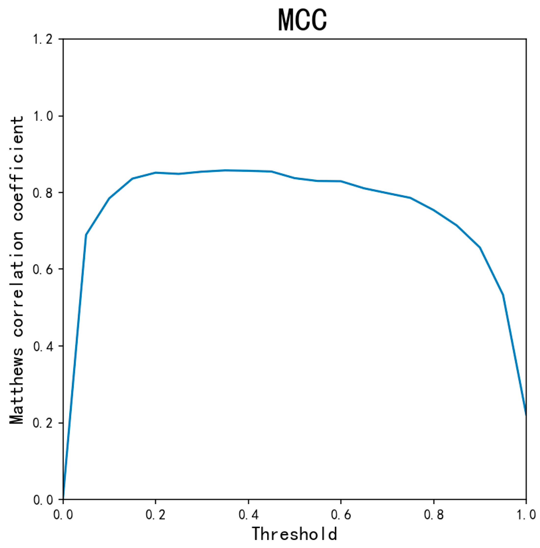
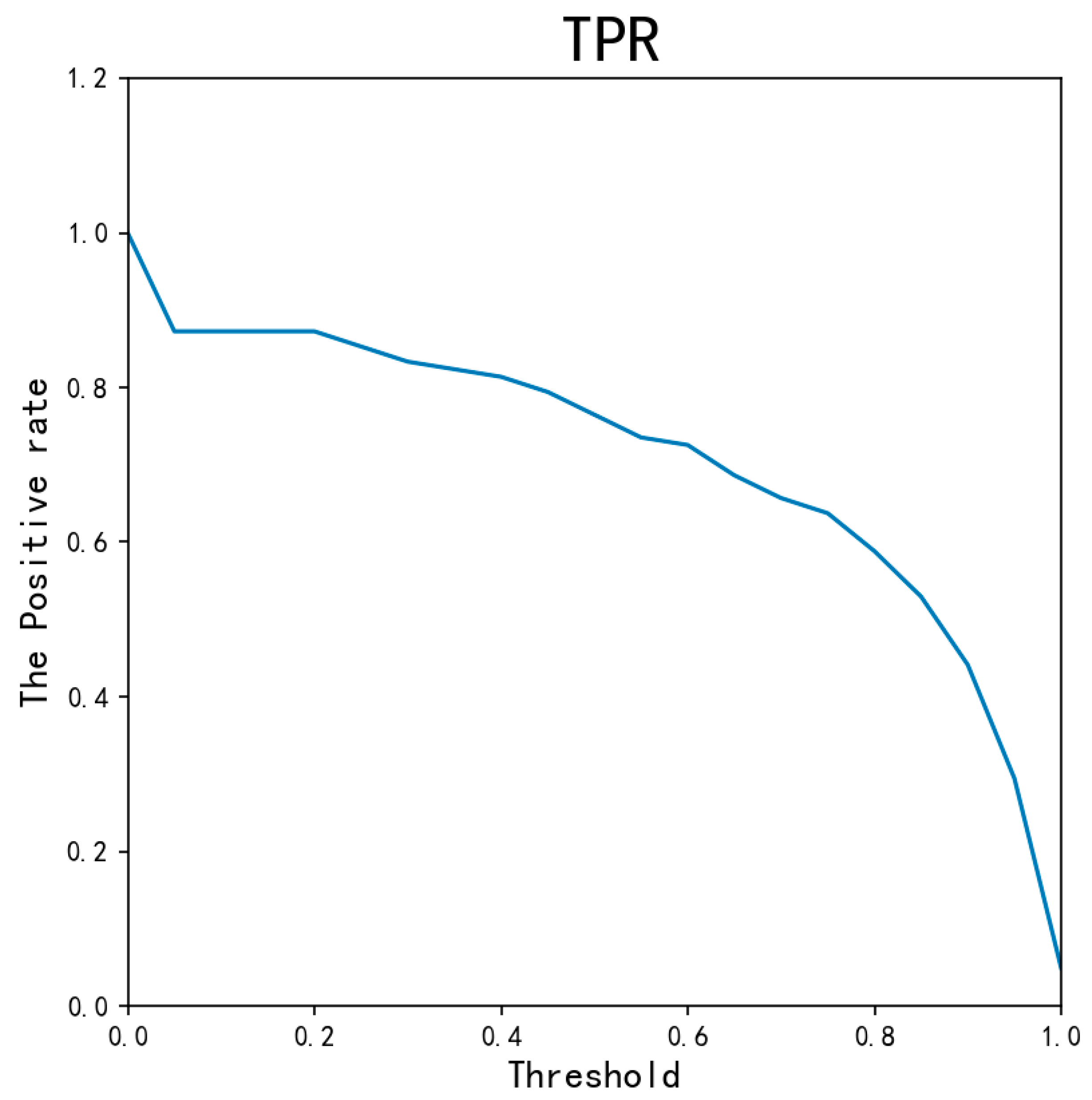
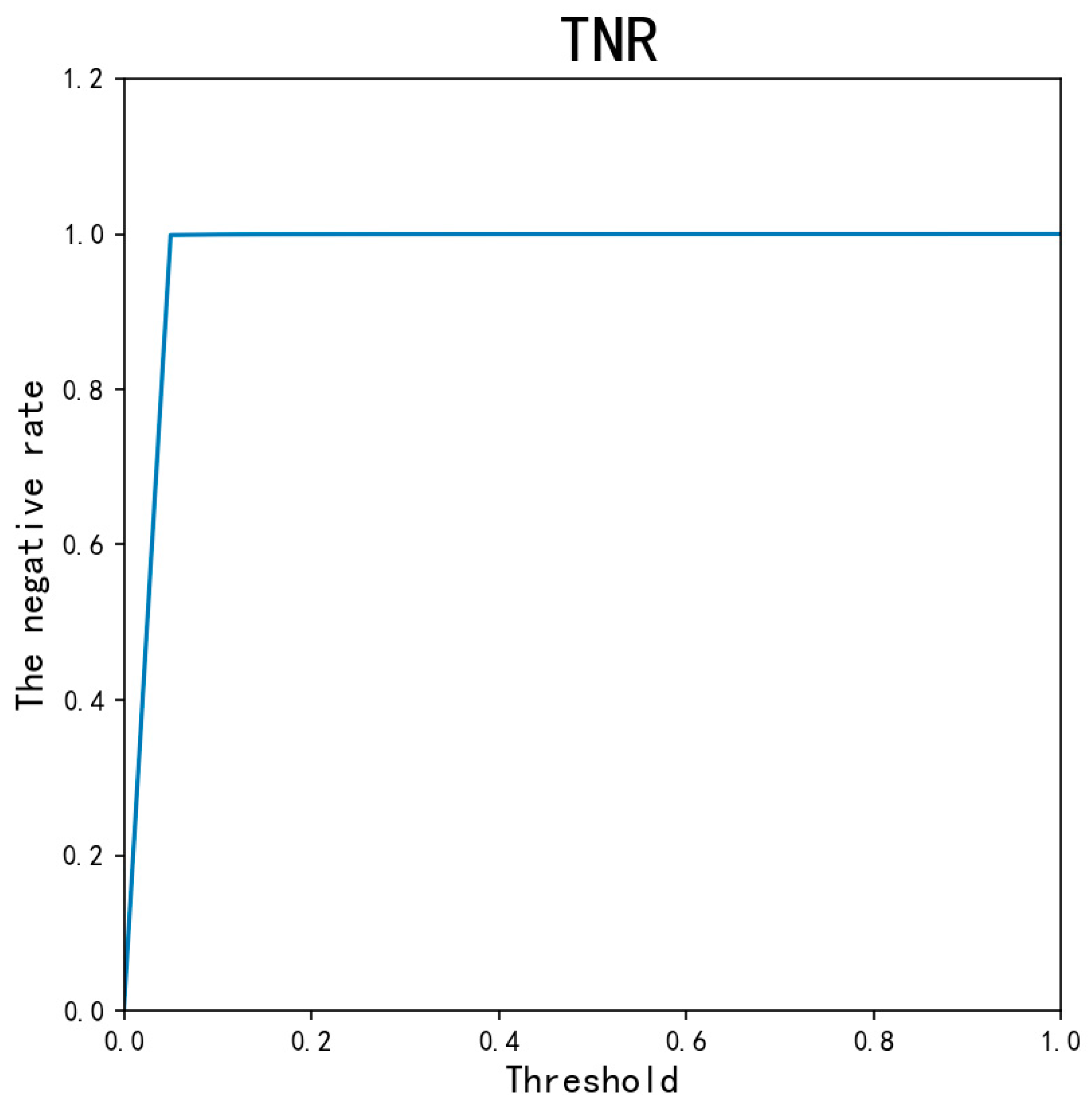
- The proposed model was evaluated using MCC, TPR, TNR, and ACC values. The experimental results indicate superior performance to that of existing models, such as KNN, LightGBM, and random forest.
2. Related Work
3. The Proposed Method
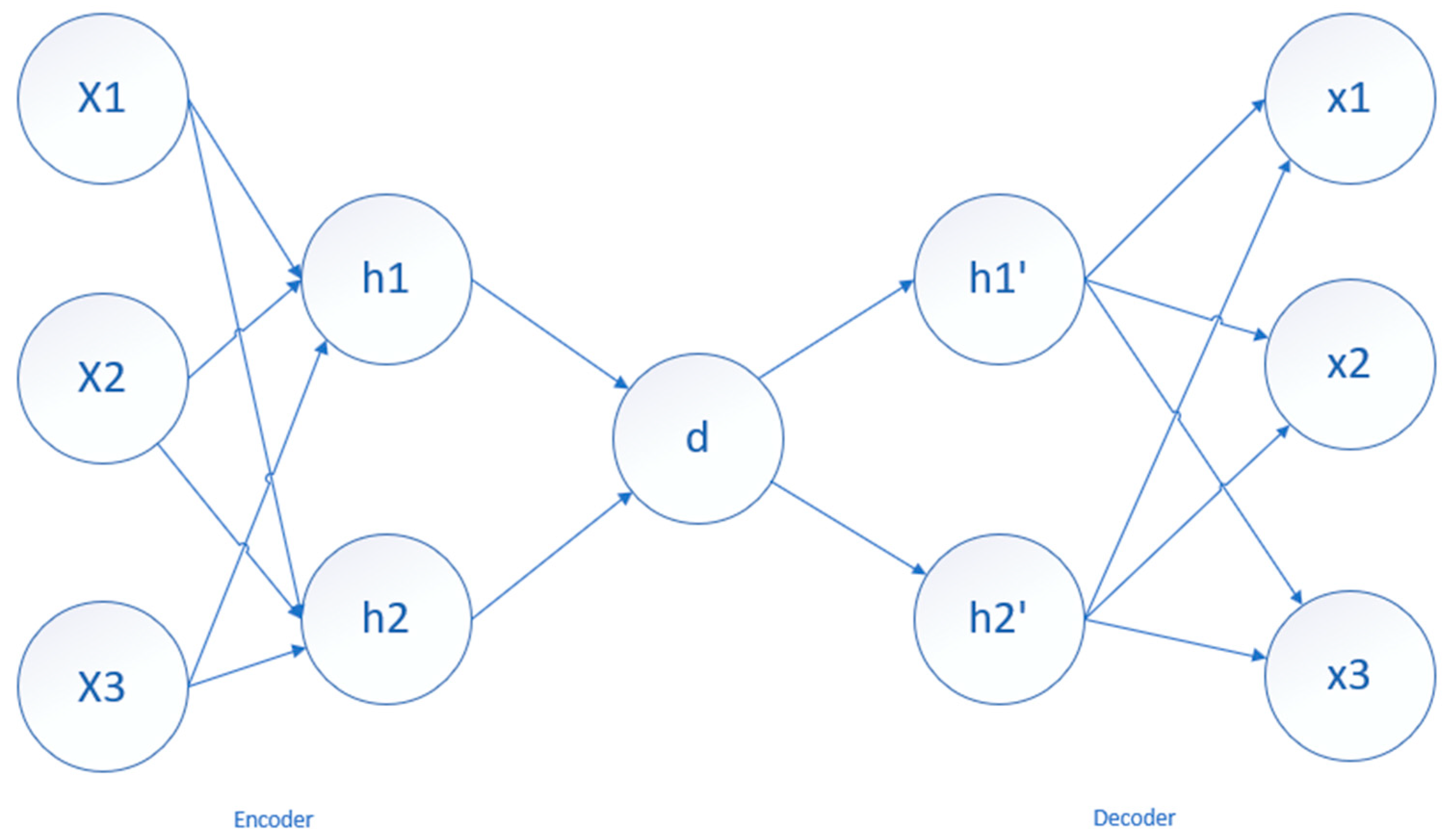
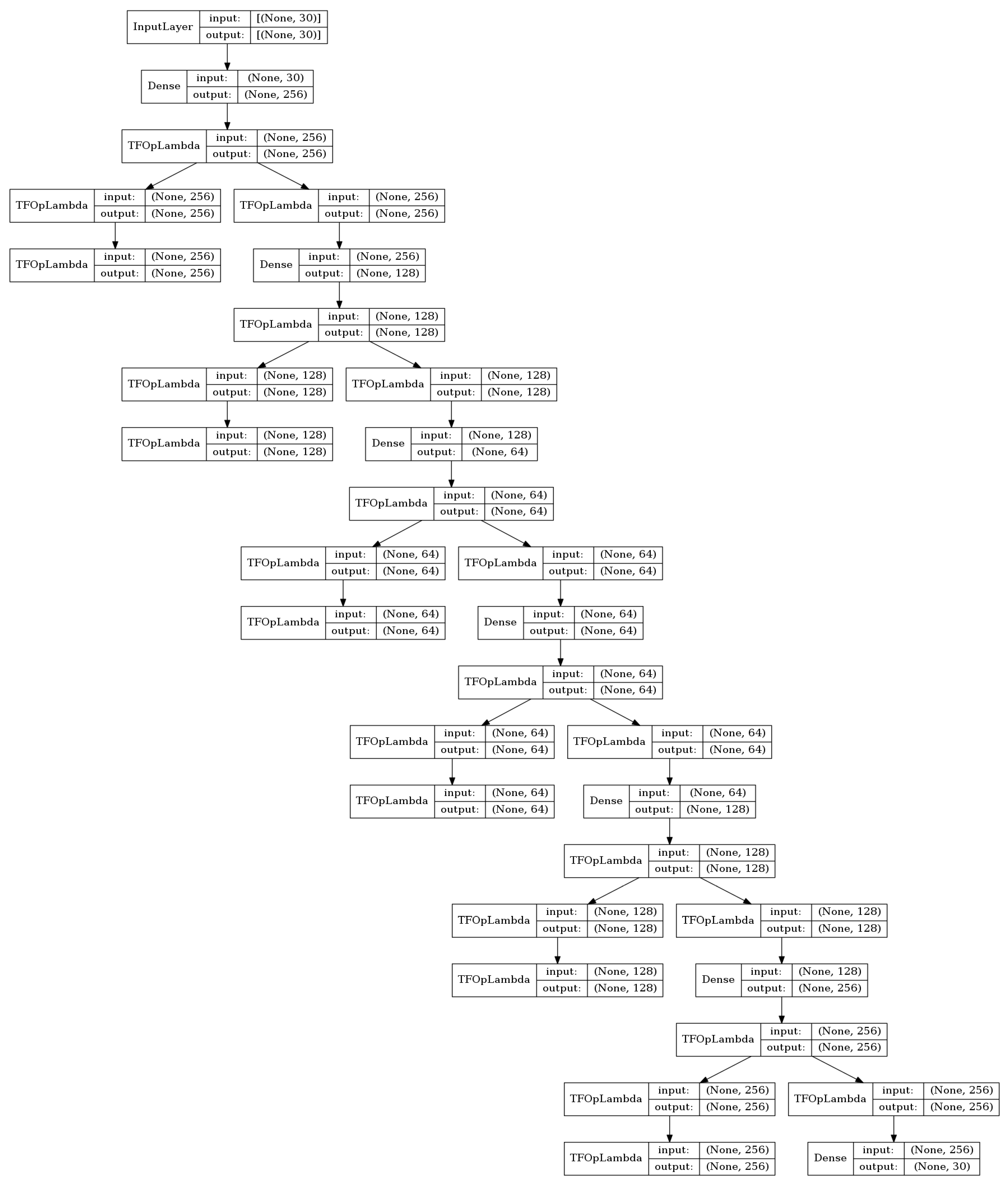
3.1. AutoEncoder
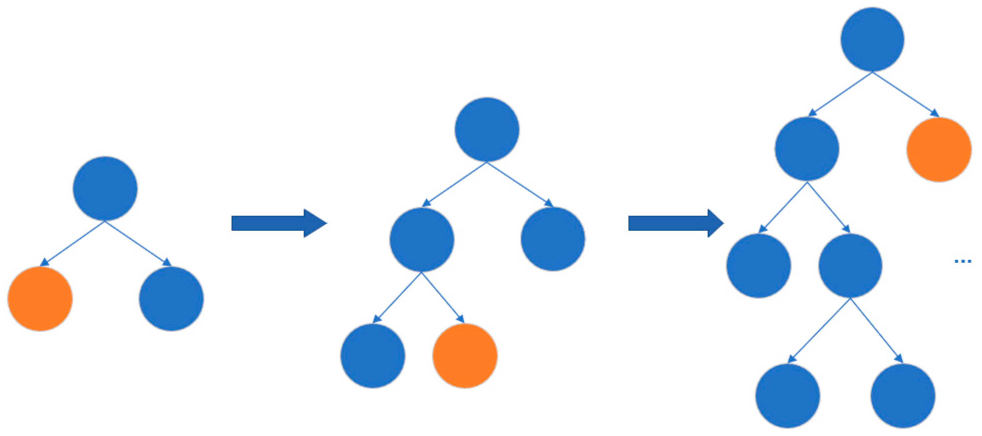
3.2. LightGBM
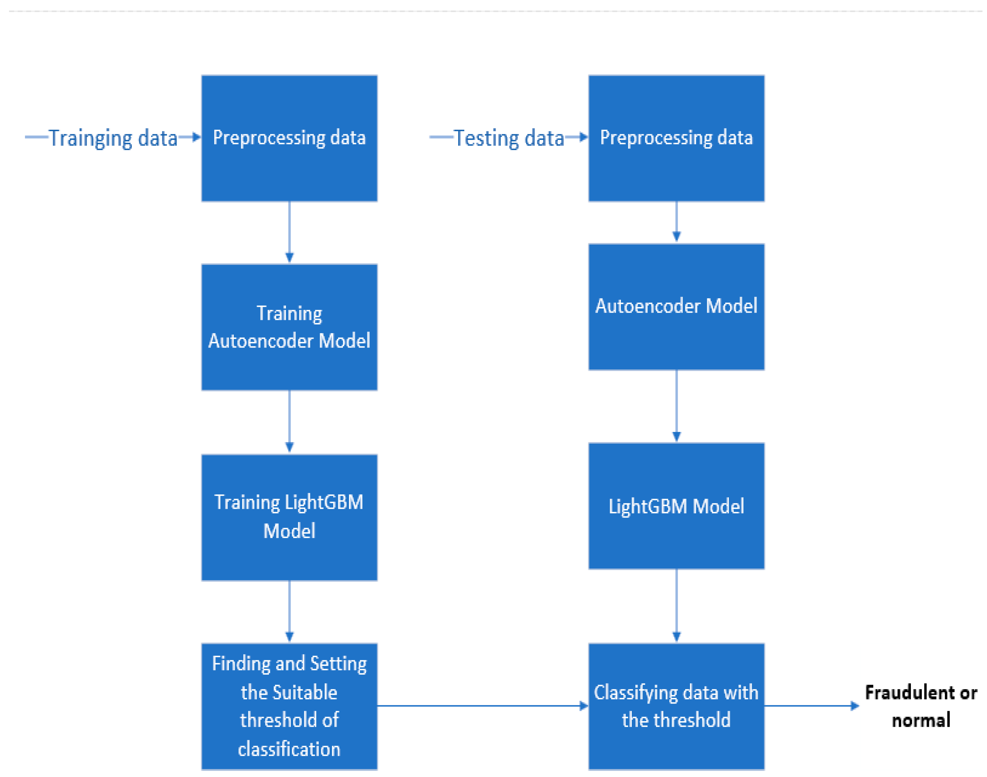
3.3. The AED-LGB Method
| Algorithm 1: AED-LGB Algorithm |
| Input: Xtrain: trainging data; Xvalidation: validation data; Xtest: test data; Output: the classification result for every test data, the result is 0 or 1, 0 represents normal and 1 represents fraudulent; |
|
4. Discussion and Experimental Results
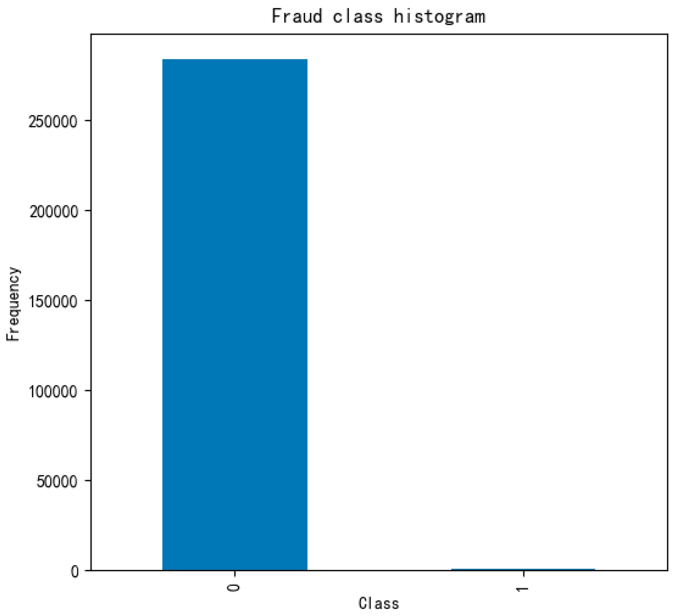
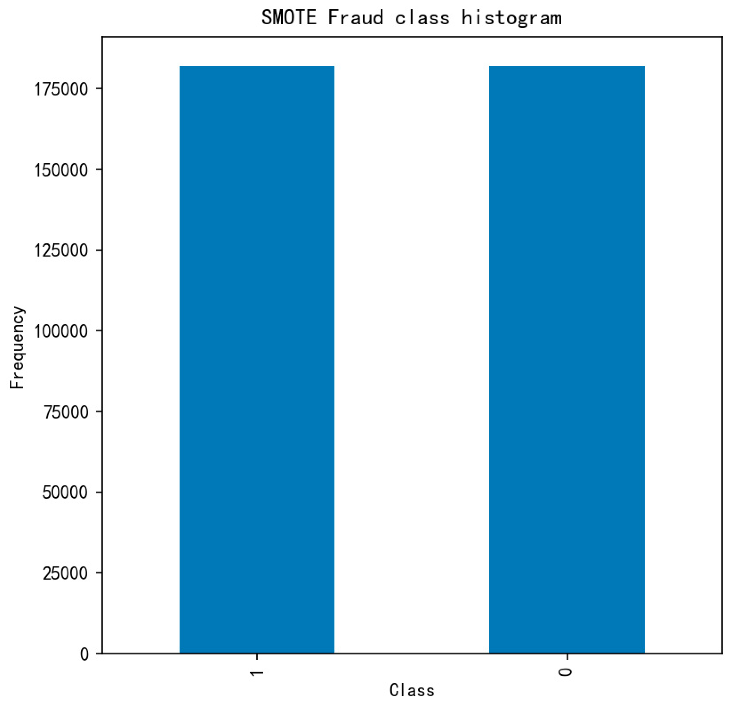
4.1. Data Pre-Processing
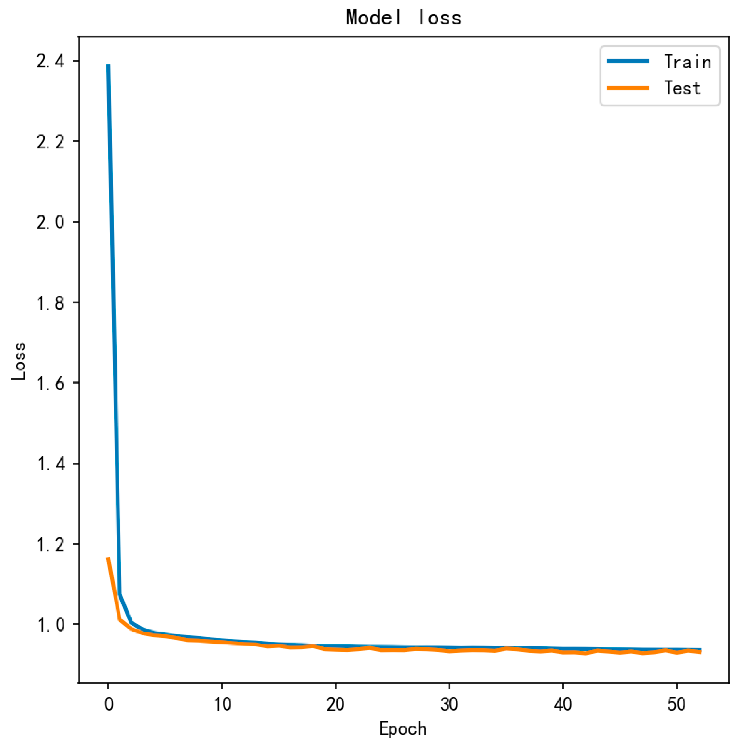
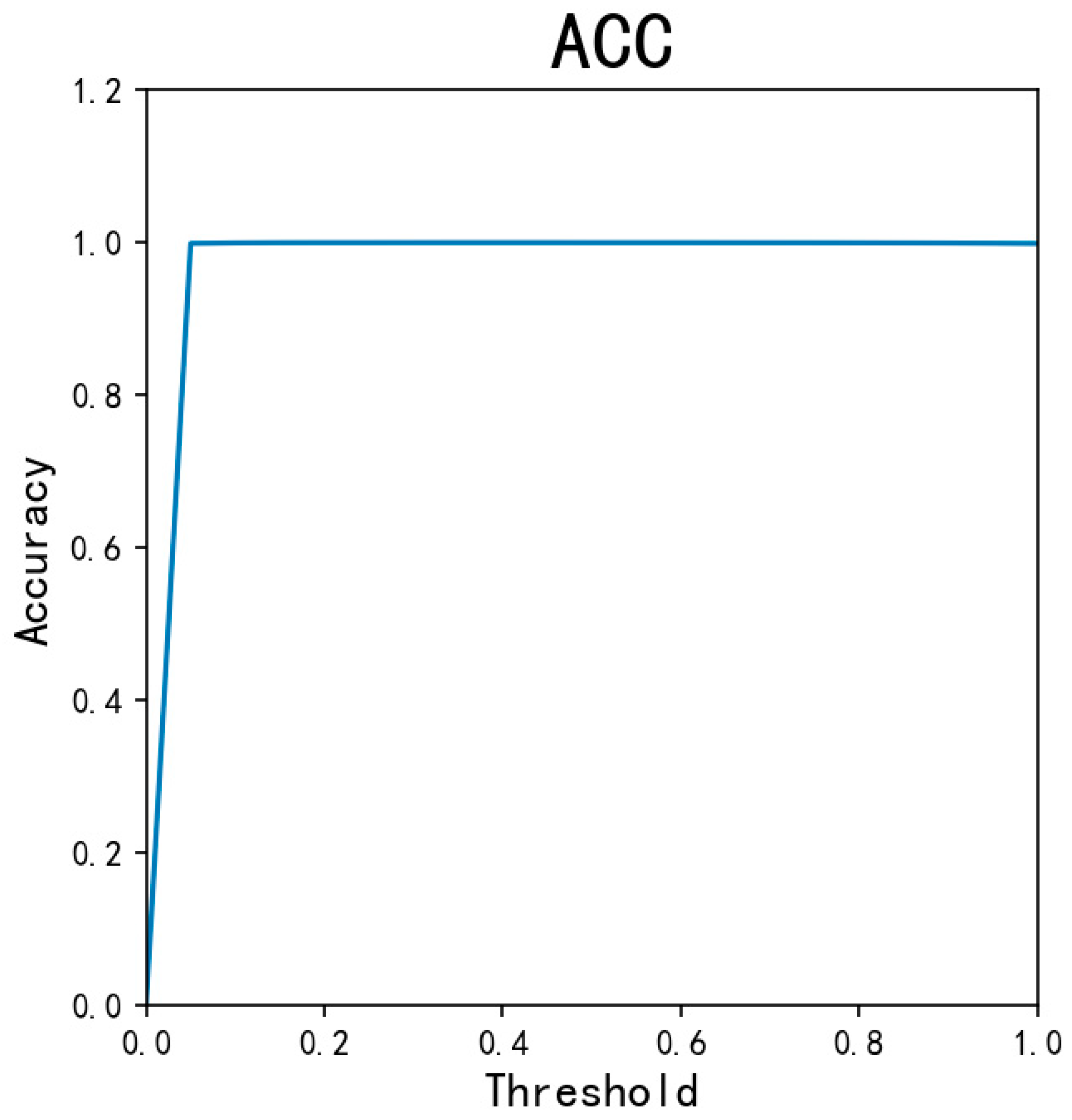
4.2. Experiment and Performance Evaluation of the AED-LGB Algorithm
4.3. Discussion and Application
5. Conclusions
Author Contributions
Funding
Data Availability Statement
Conflicts of Interest
References
- de Best, R. Credit Card and Debit Card Number in the U.S. 2012–2018. Statista. Available online: https://www.statista.com/statistics/245385/number-of-credit-cards-by-credit-card-type-in-the-united-states/#statisticContainer (accessed on 10 October 2021).
- Li, M.S.; Yang, D.; Qin, Y.H. Anti-Fraud White Paper of Digital Finance. Available online: https://www.arx.cfa/~/media/45620250D60C4DEFB081322259723D92.ashx (accessed on 31 May 2018).
- Gangopadhyay, S.; Zhai, A. CGBNet: A Deep Learning Framework for Compost Classification. IEEE Access 2022, 10, 90068–90078. [Google Scholar] [CrossRef]
- Wu, X.; Jiang, G.; Wang, X.; Xie, P.; Li, X. A Multi-Level-Denoising Autoencoder Approach for Wind Turbine Fault Detection. IEEE Access 2019, 8, 25579–25587. [Google Scholar] [CrossRef]
- Taha, A.A.; Malebary, S.J. An intelligent approach to credit card fraud detection using an optimized light gradient boosting machine. IEEE Access 2020, 8, 25579–25587. [Google Scholar] [CrossRef]
- Chen, Y.-R.; Leu, J.-S.; Huang, S.-A.; Wang, J.-T.; Takada, J.-I. Predicting default risk on peer-to-peer lending imbalanced datasets. IEEE Access 2021, 9, 73103–73109. [Google Scholar] [CrossRef]
- Dal Pozzolo, A. Adaptive Machine Learning for Credit Card Fraud Detection. Ph.D. Thesis, Université Libre de Bruxelles, Bruxelles, Belgium, 2015. [Google Scholar]
- Lucas, Y.; Portier, P.-E.; Laporte, L.; Calabretto, S.; Caelen, O.; He-Guelton, L.; Granitzer, M. Multiple perspectives HMM-based feature engineering for credit card fraud detection. In Proceedings of the 34th ACM/SIGAPP Symposium on Applied Computing, Limassol, Cyprus, 8–12 April 2019; pp. 1359–1361. [Google Scholar]
- Awoyemi, J.O.; Adetunmbi, A.O.; Oluwadare, S.A. Credit card fraud detection using machine learning techniques: A comparative analysis. In Proceedings of the 2017 International Conference on Computing Networking and Informatics (ICCNI), Lagos, Nigeria, 29–31 October 2017; pp. 1–9. [Google Scholar]
- Zhang, F.; Liu, G.; Li, Z.; Yan, C.; Jiang, C. GMM-based undersampling and its application for credit card fraud detection. In Proceedings of the 2019 International Joint Conference on Neural Networks (IJCNN), Budapest, Hungary, 14–19 July 2019; pp. 1–8. [Google Scholar]
- Ahammad, J.; Hossain, N.; Alam, M.S. Credit card fraud detection using data pre-processing on imbalanced data-Both oversampling and undersampling. In Proceedings of the International Conference on Computing Advancements, Dhaka, Bangladesh, 10–12 January 2020; pp. 1–4. [Google Scholar]
- Lee, Y.-J.; Yeh, Y.-R.; Wang, Y.-C.F. Anomaly detection via online oversampling principal component analysis. IEEE Trans. Knowl. Data Eng. 2012, 25, 1460–1470. [Google Scholar] [CrossRef]
- Wiese, B.; Omlin, C. Credit Card Transactions, Fraud Detection, and Machine Learning: Modelling Time with LSTM Recurrent Neural networks; Springer: Berlin/Heidelberg, Germany, 2009. [Google Scholar]
- Jurgovsky, J.; Granitzer, M.; Ziegler, K.; Calabretto, S.; Portier, P.-E.; He-Guelton, L.; Caelen, O. Sequence classification for credit-card fraud detection. Expert Syst. Appl. 2018, 100, 234–245. [Google Scholar] [CrossRef]
- Randhawa, K.; Loo, C.K.; Seera, M.; Lim, C.P.; Nandi, A.K. Credit card fraud detection using AdaBoost and majority voting. IEEE Access 2018, 6, 14277–14284. [Google Scholar] [CrossRef]
- Hsin, Y.-Y.; Dai, T.-S.; Ti, Y.-W.; Huang, M.-C.; Chiang, T.-H.; Liu, L.-C. Feature engineering and resampling strategies for fund transfer fraud with limited transaction data and a time-inhomogeneous modi operandi. IEEE Access 2022, 10, 86101–86116. [Google Scholar] [CrossRef]
- Naveen, P.; Diwan, B. Relative Analysis of ML Algorithm QDA, LR and SVM for Credit Card Fraud Detection Dataset. In Proceedings of the 2020 Fourth International Conference on I-SMAC (IoT in Social, Mobile, Analytics and Cloud) (I-SMAC), Palladam, India, 7–9 October 2020; pp. 976–981. [Google Scholar]
- Shirodkar, N.; Mandrekar, P.; Mandrekar, R.S.; Sakhalkar, R.; Kumar, K.C.; Aswale, S. Credit card fraud detection techniques–A survey. In Proceedings of the 2020 International Conference on Emerging Trends in Information Technology and Engineering (ic-ETITE), Vellore, India, 24–25 February 2020; pp. 1–7. [Google Scholar]
- Malini, N.; Pushpa, M. Analysis on credit card fraud identification techniques based on KNN and outlier detection. In Proceedings of the 2017 Third International Conference on Advances in Electrical, Electronics, Information, Communication and bio-Informatics (AEEICB), Chennai, India, 27–28 February 2017; pp. 255–258. [Google Scholar]
- Pumsirirat, A.; Liu, Y. Credit card fraud detection using deep learning based on auto-encoder and restricted boltzmann machine. Int. J. Adv. Comput. Sci. Appl. 2018, 9, 18–25. [Google Scholar] [CrossRef]
- Zamini, M.; Montazer, G. Credit card fraud detection using autoencoder based clustering. In Proceedings of the 2018 9th International Symposium on Telecommunications (IST), Tehran, Iran, 17–19 December 2018; pp. 486–491. [Google Scholar]
- Krishna, M.V.; Praveenchandar, J. Comparative Analysis of Credit Card Fraud Detection using Logistic regression with Random Forest towards an Increase in Accuracy of Prediction. In Proceedings of the 2022 International Conference on Edge Computing and Applications (ICECAA), Tamilnadu, India, 13–15 October 2022; pp. 1097–1101. [Google Scholar]
- Wulsin, D.; Blanco, J.; Mani, R.; Litt, B. Semi-supervised anomaly detection for EEG waveforms using deep belief nets. In Proceedings of the 2010 Ninth International Conference on Machine Learning and Applications, Washington, DC, USA, 12–14 December 2010; pp. 436–441. [Google Scholar]
- Zhou, C.; Paffenroth, R.C. Anomaly detection with robust deep autoencoders. In Proceedings of the 23rd ACM SIGKDD International Conference on Knowledge Discovery and Data Mining, Halifax, NS, Canada, 13–17 August 2017; pp. 665–674. [Google Scholar]
- Chalapathy, R.; Menon, A.K.; Chawla, S. Anomaly detection using one-class neural networks. arXiv 2018, arXiv:1802.06360. [Google Scholar]
- Wasikowski, M.; Chen, X.-w. Combating the small sample class imbalance problem using feature selection. IEEE Trans. Knowl. Data Eng. 2009, 22, 1388–1400. [Google Scholar] [CrossRef]
- Wang, M.; Zhao, M.; Chen, J.; Rahardja, S. Nonlinear unmixing of hyperspectral data via deep autoencoder networks. IEEE Geosci. Remote Sens. Lett. 2019, 16, 1467–1471. [Google Scholar] [CrossRef]
- Liang, W.; Luo, S.; Zhao, G.; Wu, H. Predicting hard rock pillar stability using GBDT, XGBoost, and LightGBM algorithms. Mathematics 2020, 8, 765. [Google Scholar] [CrossRef]
- Hashemi, S.K.; Mirtaheri, S.L.; Greco, S. Fraud Detection in Banking Data by Machine Learning Techniques. IEEE Access 2022, 11, 3034. [Google Scholar] [CrossRef]
- Camacho, L.; Douzas, G.; Bacao, F. Geometric SMOTE for regression. Expert Syst. Appl. 2022, 2022, 116387. [Google Scholar] [CrossRef]
- Misra, D. Mish: A self regularized non-monotonic activation function. arXiv 2019, arXiv:1908.08681. [Google Scholar]
- Zhu, Q. On the performance of Matthews correlation coefficient (MCC) for imbalanced dataset. Pattern Recognit. Lett. 2020, 136, 71–80. [Google Scholar] [CrossRef]


| Time | V1 | V2 | V3 | V4 | V5 | V28 | Amount | Class |
|---|---|---|---|---|---|---|---|---|
| 0 | −1.359807134 | −0.072781173 | 2.536346738 | 1.378155224 | −0.33832077 | −0.021053053 | 149.62 | 0 |
| 406 | −2.312226542 | 1.951992011 | −1.609850732 | 3.997905588 | −0.522187865 | −0.143275875 | 0 | 1 |
| 472 | −3.043540624 | −3.157307121 | 1.08846278 | 2.288643618 | 1.35980513 | 0.035764225 | 529 | 1 |
| Models | ACC | TPR | TNR | MCC |
|---|---|---|---|---|
| AED-LGB (threshold = 0.2) | 0.9993 | 0.8039 | 0.9997 | 0.8506 |
| AED-LGB (threshold = 0.05) | 0.9987 | 0.8929 | 0.993 | 0.773 |
| AED-LGB-SMOTE (threshold = 0.70) | 0.9970 | 0.8275 | 0.9973 | 0.5574 |
| Models | ACC | TPR | TNR | MCC |
|---|---|---|---|---|
| AED-LGB (threshold = 0.2) | 0.9993 | 0.8039 | 0.9997 | 0.8506 |
| AED-LGB (threshold = 0.05) | 0.9987 | 0.8929 | 0.9932 | 0.773 |
| KNN | 0.9691 | 0.8835 | 0.9711 | 0.5903 |
| LightGBM | 0.9696 | 0.8529 | 0.9995 | 0.8100 |
| Random Forest | 0.9583 | 0.8025 | 0.9989 | 0.6902 |
Disclaimer/Publisher’s Note: The statements, opinions and data contained in all publications are solely those of the individual author(s) and contributor(s) and not of MDPI and/or the editor(s). MDPI and/or the editor(s) disclaim responsibility for any injury to people or property resulting from any ideas, methods, instructions or products referred to in the content. |
© 2023 by the authors. Licensee MDPI, Basel, Switzerland. This article is an open access article distributed under the terms and conditions of the Creative Commons Attribution (CC BY) license (https://creativecommons.org/licenses/by/4.0/).
Share and Cite
Du, H.; Lv, L.; Guo, A.; Wang, H. AutoEncoder and LightGBM for Credit Card Fraud Detection Problems. Symmetry 2023, 15, 870. https://doi.org/10.3390/sym15040870
Du H, Lv L, Guo A, Wang H. AutoEncoder and LightGBM for Credit Card Fraud Detection Problems. Symmetry. 2023; 15(4):870. https://doi.org/10.3390/sym15040870
Chicago/Turabian StyleDu, Haichao, Li Lv, An Guo, and Hongliang Wang. 2023. "AutoEncoder and LightGBM for Credit Card Fraud Detection Problems" Symmetry 15, no. 4: 870. https://doi.org/10.3390/sym15040870
APA StyleDu, H., Lv, L., Guo, A., & Wang, H. (2023). AutoEncoder and LightGBM for Credit Card Fraud Detection Problems. Symmetry, 15(4), 870. https://doi.org/10.3390/sym15040870