Article

Towards a Dynamic Compartmental Model of a Lamellar Settler

Faculty of Water Science, University of Public Service, 6500 Baja, Hungary
Symmetry 2023, 15(4), 864; https://doi.org/10.3390/sym15040864
Submission received: 11 March 2023 / Revised: 1 April 2023 / Accepted: 4 April 2023 / Published: 5 April 2023

Abstract

:
Lamellar settlers are widely used in solid separation due to their relative high surface area paired with a small tank volume. Settlers exposed to high load variations may change their settling properties based on the variation of the flow pattern. Applying the critical point theory and coherent structure concept, a flow topology analysis was performed with the help of computational fluid dynamic simulations. The compartments were determined by the fluid flow, and the dynamic behavior of the compartments was taken into account. Under normal diurnal load variation, the architecture of the compartments did not change, in contrast to the mass transport between the zones, whereas the sludge removal process made significant changes in the architecture. The results showed two main flow zones with significant internal recirculation in the first zone. The hydraulic surface loading was examined in each zone, and the study revealed that the actual hydraulic load could be from 1.5 to 4.5 times much higher than that in individual zones due to recirculation eddies in the reactor tanks. The design hydraulic loading rate did not consider the local flow pattern. The discrete phase model approximation provided acceptable results, and the extent of the recirculation zone changed stepwise with different loads.

1. Introduction

The removal of solid matter, including both organic and inorganic components, is a crucial aspect of water and wastewater treatment processes. This solid separation step is responsible for reducing the pollutant load of downstream equipment by removing a significant portion of the contaminants present in raw wastewater [1]. The efficiency of this separation process is dependent on various factors, including the characteristics of the raw water, such as the solid content and particle size distribution, as well as the hydrodynamic conditions and environmental factors present [2].
From a hydrodynamic perspective, the overall efficiency of the separation process is influenced by several key factors, including the hydraulic load, the density difference between the solid and the liquid phases, and the viscosity of the liquid. Additionally, the gravitational acceleration is also an important factor to consider. At the local level, the presence of turbulence and shear forces could also play a role in the efficiency of the solid–liquid separation process [3]. The shear rate required for optimal separation can vary depending on the characteristics of the particles being separated. Flocculating particles, which tend to aggregate, require a lower shear rate to allow for particle aggregation and settling than non-flocculating particles, which do not aggregate as easily. Additionally, the desired shear rate can vary depending on the specific stage of the separation process: a low shear rate is desirable during the sedimentation stage to allow for the particles to settle out of the liquid. Undesirable shear can negatively impact the efficiency of the separation process by causing the formation of small flocs which are more difficult to settle, destabilizing emulsions and decreasing the efficiency of flocculating agents. Additionally, high shear rates can cause the particles to break apart, leading to a decrease in separation efficiency [4].
Local turbulence parameters such as turbulent viscosity and turbulent dissipation have also an effect on the phase separation efficiency. Turbulent viscosity originates from the rate of strain in the flow; with a high virtual viscosity, the flow resistance to the settling motion increases, and thus the separation efficiency decreases. In contrast, high turbulent dissipation refers to a high local mixing intensity and promotes flocculation and settling [5].
Furthermore, the flow field topology within a process unit could provide information on the hydrodynamic behavior. A topology that promotes the formation of eddies and vortices could increase the particle collision and, thus, the flocculation, which may lead to higher settling rates [6]. An opposite effect could be observed if the flow is highly turbulent, or shear layers are developed [7]. The flow topology can change over time as the flow evolves and the conditions in the liquid change [8]. The fluid structure within a sedimentation process can be affected by variations in the load conditions, such as changes in the flow rate, particle size, and concentration, and properties of the liquid. The optimal design of the sedimentation process should take into account these potential variations and adjust accordingly. Such adjustments may include the geometry of the tank, with a focus on the radial flow, the positioning of inlets and outlets, the implementation of baffles, and the incorporation of inclined plates.
The use of inclined plates increases the total surface area available for solid–liquid separation, thus reducing the required size of the process unit while maintaining efficiency [9]. The removal of settled sludge can be performed in a continuous or in a batch manner. The discharge flow from the sludge removal process may also have an impact on the flow pattern through backpropagation [10].
Computational fluid dynamics (CFD) could be a helpful tool to reveal the possible small-scale flow phenomena within the process unit and optimize the hydrodynamic conditions with variable loads. Many efforts have been made in the numerical modelling of the fluid flow in lamella settlers [11]. Earlier studies widely used single-phase flow models because they were computationally efficient and produced accurate results [12]. With recent advancements in computing power, researchers have shifted to using multiphase models to more accurately model sedimentation [13]. The Euler–Euler or Euler–Lagrange method can be used to simulate the multiphase flow observed in settling tanks. In the near future, a full-scale, realistic transient simulation of a settling tank that includes sub-models for factors such as flocculation, sludge rheology, and thermal conditions will be possible [14].
As for the transport processes, the approaches to describing reactors range from the simplest, treating the entire reactor as an ideal one, to the most detailed, using CFD with fine discretization. The intermediate approach considers the reactor as a combination of some ideal reactors, the so-called systemic approach or the compartmental method, where all compartments are assumed to be perfectly mixed. The compartments can be defined purely by geometry or by a certain flow characteristic [15].
Coherent structures in a flow are patterns that are distinguished from the surrounding turbulent or chaotic flow by their relative stability and regularity. These can be characterized by strong gradients in velocity and/or vorticity [16]. Coherent structures in a flow can exhibit both symmetry and asymmetry. It depends on the specific flow and the structures that are observed within it. Some coherent structures, such as vortices or jets, can be symmetric in shape or behavior, while others can be asymmetric. For example, a symmetric vortex will have a circular shape, and the fluid motion within the vortex will be rotationally symmetric about its central axis, while an asymmetric vortex will have an irregular shape, and the fluid motion within it will not be rotationally symmetric. It is also possible for a flow to have both symmetric and asymmetric coherent structures present at the same time [17]. The identification could apply the linear combination of the proper orthogonal decomposition (POD) modes of vorticity [18] or criterion-based assessments [19].
Based on the coherent structures detected in a flow field, zones with similarity could be delineated. There are several techniques to separate compartments. The most common is the visualization approach, where the streamlines delimit the regions, whereas a spectral analysis decomposes the flow into various frequency components and identifies the coherent structures that are associated with a certain frequency range [20]. While Lagrangian methods take into account particle tracking, the Eulerian approach applying a topological analysis originates from fixed-point theories [21]. Both are widely used in steady-state conditions, but the dynamic behavior of the delineated zones is rarely investigated. There are examples of Artificial Intelligence (AI)-based methods in vortex detection [22], especially originating from their image recognition capability, but the mechanistic models have an advantage in terms of robustness and transparency.
The objective of this study was to predict the hydrodynamic conditions of an inclined/lamellar settler utilizing compartmental modeling and to study the compartments’ configuration and inter-compartmental mass transfer at various hydraulic loads. Although CFD-based research is not novel in this field, the innovation of this study lies in the compartmentalization approach and the consideration of the compartments’ dynamics. The compartments were defined using critical point theory and dynamic behavior, and the evolution of the volume of the compartments based on the hydraulic load incoming to the settler was investigated, which to the authors’ knowledge, has not been investigated to date.

2. Materials and Methods

2.1. Flow Field Calculation

The governing equations of CFD simulations are usually based on the Navier–Stokes equations, which describe the motion and behavior of fluids. These equations can be expressed as a set of partial differential equations (PDEs) and can be solved using numerical methods. For 3D steady-state incompressible flows, applying Reynolds averaging and Einstein notation in Cartesian coordinates, the following form was used for continuity Equation (1) and the three components of the momentum equations (Equation (2)).
u ¯ i x i = 0
ρ u j ¯ u ¯ i x j = ρ f ¯ i + x j p ¯ δ i j + μ u ¯ i x j + u ¯ j x i ρ u i u j ¯
where i, j: x, y, z are the Cartesian coordinates, u is the velocity, ρ is the fluid density, f is the external force, g is the gravitational acceleration, p is the pressure, δ is the Kronecker delta, µ is the dynamic viscosity.
The left-hand side of Equation (2) contains the convective term, while the right-hand side contains the external force, pressure gradient, diffusion term, and virtual stress from the Reynolds averaging. For turbulence closure, the k-ω model was applied, which assumes isotropy and near-wall treatment and is well-suited for flows with strong pressure gradients, such as those found in boundary layers and separated flows [23]. As for the numerical approach, the discretization scheme followed the upwind scheme. Second-order Taylor-series expansion was applied in order to reduce the numerical diffusion [24]. The general SIMPLE scheme (Semi-Implicit Method for Pressure-Linked Equations) was solved for pressure–velocity coupling. Steady-state flow field separate simulations for various incoming flows were performed. The convergence criteria were to achieve that the residuals of the governing equations between two iterative steps were minimized.
Lagrangian particle tracking in the Eulerian flow field involved following the movement of particles in a fluid as they were carried along by the flow. This was carried out by tracking the position and velocity of each individual particle over time. There was only a one-way coupling between the solid particles and the fluid flow; the particles were assumed to be small enough that their motion could be approximated as being affected by the surrounding fluid, but not significantly altering the fluid’s flow. The random walk approach was used to capture the turbulent properties [25]. The mathematical formulation of Lagrangian particle tracking follows the force balance on the particle:
m p d u p d t = 1 2 ρ f C D u ¯ u p u ¯ u p A p + ρ p ρ f g V p
where mp is the particle mass, Vp is the particle volume, Ap is the particle surface perpendicular to the movement, up is the particle velocity, u is the flow velocity, ρp is the particle density, ρf is the fluid density, CD is the drag coefficient calculated as follows:
C D = 24 R e 1 + 0.15 R e 0.687 ,   R e < 1000 0.44 ,   R e > 1000
where Reynolds number (Re) can be determined as follows:
R e = ρ f d p u ¯ u p μ
where dp is the particle diameter.
To predict the dispersion due to turbulence, the Gaussian-distributed random velocity fluctuations were calculated as follows:
u i = ϑ u i 2 ¯
where ϑ is a normally distributed random number. The characteristic eddy lifetime (τe) was then calculated applying ω from the turbulence model, as follows [25]:
τ e = 0.3 ω
The methodology of the residence time distribution (RTD) analysis was based on the author’s previous work [26], in which a two-phase flow was assumed, where both phases of the fluid had the same material properties, and the only difference between the phases was their spatial and temporal distribution. As an initial condition, the entire domain was full with phase 1 using an a priori steady-state flow simulation. At a given time (t = 0 s), the simulation was set to transient, and the input boundary condition was changed so that only phase 2 was discharged at the same rate as phase 1. As time progressed, phase 1 was displaced because there was no refill through the input boundary condition, and the rate of this process could be tracked by the volume fraction (α) scalar variable:
V q = α q d V
q = 1 n α q = 1
where α is the volume fraction of the q-th phase.
The volume fraction as a function of time could be depicted at the outlet boundary, which represents the so-called F-curve in RTD analysis [27]. The cumulative function of the volume fraction applied the normalized time as follows [28]:
θ = t t ¯
where θ is the normalized time, and t ¯ is the average time.

2.2. Coherent Structure Detection and Compartmentalization

The critical point theory provides a useful framework for understanding the complex behavior of fluid flows with coherent structures. The critical point is a point where the gradient of the velocity field is zero. The velocity field changes from a region of acceleration to a region of deceleration, leading to the formation of vortices and other coherent structures in the flow. By the help of the local velocity gradient tensor, the behavior of the fluid in the near zone of critical points could be outlined by applying the eigenvalues and eigenvectors of the matrix. The Jacobian matrix for a two-dimensional vector (u, v) is
A = u i x i x i , 0 = u x u y v x v y x 0 , y 0
The eigenvalues of the A matrix can be calculated using the following equation:
d e t   A λ I = 0
where λ is the eigenvalue, and I is the unity matrix.
If the real part of the eigenvalue is negative (Re < 0), it creates an attractive force, whereas if it is positive, it causes a repulsive force (Re > 0). On the other hand, the imaginary part (Im) of the eigenvalue results in a rotation of the vector field around the critical point. If there is an imaginary eigenvalue, the vector field around the critical point will be entirely rotational. This categorization is based on the existence of the imaginary part and the sign of the real part of the complex eigenvalue based on Table 1 [29].
By examining a steady-state flow field, streamlines were used to identify critical points on visual and intuitive construct compartments. The separatrices served as boundaries for each compartment, and in turbulent flows, mass exchange occurred between zones. The fluxes through the compartments were calculated to establish the architecture of the compartment model, based on a one-phase steady-state flow.

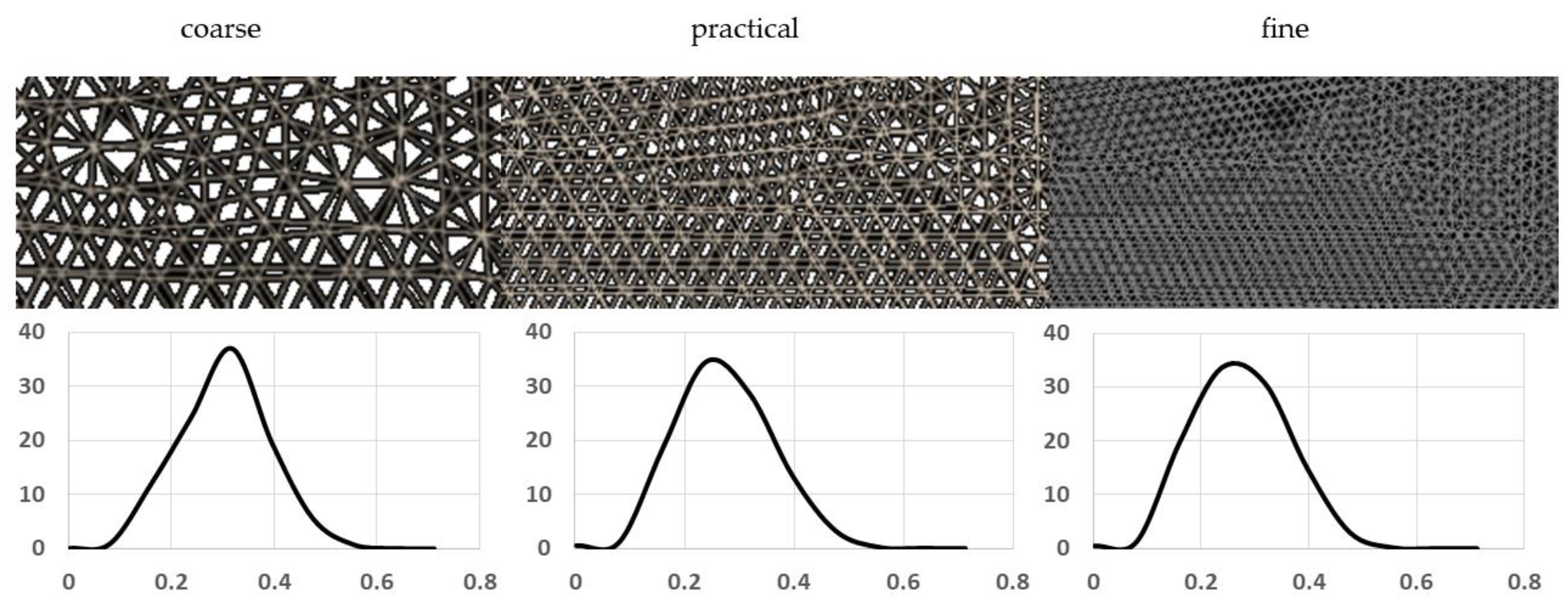
2.3. Mesh Independence Test and Validity of the Model
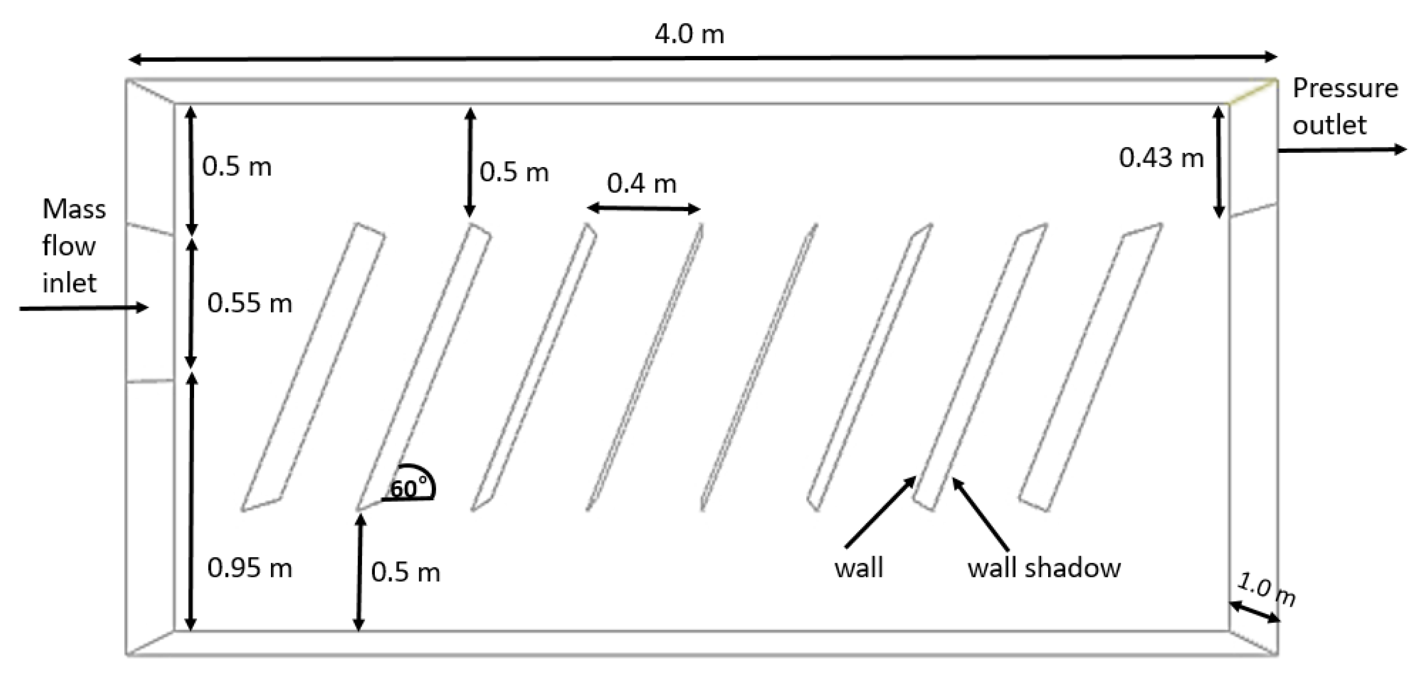
The goal of the mesh independence analysis was to investigate whether the further refinement of the grid size could significantly improve the accuracy of the results. The test started with a coarse grid and proceeded with a gradual increase of the number of cells or elements in the mesh. As a result, coarse, practical, and fine meshes were created with cell numbers of 87,126, 348,523, 1,349,220, respectively (see details in Figure 1).
The error (ε) could be estimated as follows:
ε = φ f i n e φ p r a c t i c a l r p 1
where φ is the characteristic variable for the flow, r refers to the aspect ratio of the mesh element size, and p is the order of the convergence calculated as follows:
p = log r φ p r a c t i c a l φ c o a r s e φ f i n e φ p r a c t i c a l

2.4. Model Setup

Inclined plates were placed in a rectangular channel in order to increase the settling area. The basis of the geometry and the arrangement was published in Dao et al. (2019) [30], taking into consideration the erratum by the authors published in 2020 [30]. The simulation domain had a length of 4.0 m, a height of 2.0 m, and a width of 1.0 m. Eight lamellae were placed in the simulation domain as Figure 2 shows. As for the boundary conditions, mass flow at the inlet and atmospheric pressure at the outlet were set. The inclined plates were walls, the sides of the channel had symmetry boundaries, and besides the free surface, the rest bordering surfaces were no-slip walls.
The hydraulic surface loading rate (HLR) can be calculated by dividing the flow discharge by the total surface area of the settling tank surface and the horizontal projection area of the lamellae as follows:
H L R = Q A 0 + n A L
where Q is the flow discharge, A0 is the settling tank surface area, n is the number of the lamellae, AL is the surface area of one lamella. Steady-state runs were calculated for various scenarios based on the hydraulic surface loading rate (see Table 2), taking into account the actual operational conditions of a lamellar settler.
Once the Eulerian flow fields had been calculated for each scenario, particles were introduced into the flow, and their movement was monitored. The settling velocity of the particles ranged from 0.24 to 0.80 mm/s, with an even distribution as described in reference [30]. At the boundaries, the particles either escaped through the outlet, which was reflected in the wall shadow zone, or became trapped in the wall zone of the lamellae or at the bottom [31]. The efficiency of particle separation was determined using the following formula:
η = N i n j e c t N u n f i n i s h e d N e s c a p e N i n j e c t N u n f i n i s h e d
where η is the particle separation efficiency, and N is the number of particles. The number of unfinished particles refers to those particles whose fate could not be determined within the designated timeframe. Literature data were used to verify the flow model and compare the efficiency of particle transport and sedimentation.

3. Results and Discussion

3.1. Flow Field and Mass Transport Calculation and Validation

A grid independence analysis was conducted using the average flow during dry weather condition. The integral-averaged velocity magnitudes were determined to be 2.92 × 10⁻⁴, 2.85 × 10⁻⁴, and 2.83 × 10⁻⁴ for the coarse, practical, and fine meshes, respectively. As a result, the error was around 10−8, which could be considered negligible and is likely attributable to rounding.
For each of the four loading scenarios, an analysis of the residence time was conducted, and the surface average volume fraction at the outlet was measured. As time progressed, an increasing amount of fluid from phase 2 reached the outlet. Figure 3 shows the cumulative function (F-curve) for each scenario. The x-axis displays the normalized time.
Starting from time zero, a tracer introduced into the system appeared at different times at the outlet section depending on the hydraulic surface load. For a hydraulic loading rate (HLR) of 1 m/h or greater, it represented 0.36–0.4 of the average residence time, while at low flow rates, it reached a value of approximately 0.54. This was due to slower water movement, lower turbulence, and more dominant plug flow. At the outlet section, the original fluid and tracer could be measured in roughly equal proportions after about 50% of the average residence time had elapsed (HLR = 2 m/h) and in 65% of the other loading scenarios. After the average residence time had passed, the detectable tracer phase ratio varied widely, ranging from 0.68 to 0.83, indicating that the flow pattern varied depending on the HLR. At twice the average residence time, the tracer ratio was between 0.88 and 0.92, while at relative residence times greater than 2.5, the detectability of phase 2 was similar regardless of the HLR. The formation of stable dead zones might account for this, which could not be eliminated even with higher water flow rates. Mass and energy transport between the dead zones and the main flow were solely due to turbulent diffusivity. The study conducted by Dao et al. [30] found that the tracer reached the outlet at θ = 0.35, while the value at θ = 0.53 was associated with alpha = 0.1, indicating good consistency between the present study and the reference cited.
Lagrangian particle tracking was applied to the a priori calculated Eulerian flow field to estimate the separation efficiency. In other words, discrete phase modelling was applied as detailed in the Materials and Methods section. The separation efficiency was compared with the work of Dao et al. [30], who had used the algebraic slip multiphase model and treated the solid phase as a continuum. As shown in Table 3, where the comparison was available, the two different approaches were in reasonable agreement. The deviation was calculated from the difference between the literature data and the actual simulation results, normalized by the actual simulation.
Lagrangian particle tracking underestimated the separation efficiency, which might be due to the boundary condition set at the lamellar zone, since the shadow zones could reflect the total particle mass back to the fluid flow.

3.2. Coherent Structure Detection

To detect the coherent structure, the first step was to reduce the dimensionality of the flow. This involved comparing the volume-averaged velocity magnitudes and the velocity component perpendicular to the main stream in each scenario, as shown in Table 4.
As shown in Table 4, the velocity magnitude was nearly four orders of magnitude higher than the velocity component perpendicular to the flow direction. Cross-stream dispersion was negligible and did not increase linearly with the increasing load. This implies that, for creating compartment models, it was sufficient to project the streamlines onto a two-dimensional plane and determine the critical points based on that. The turbulent kinetic energy and the dissipation rate increased with the hydraulic loading rate, together with the higher turbulent viscosity, leading to a higher dispersion of the particles.
The goal was not to map out all critical points available, but to locate the locations that were significant for settling and material flows. Therefore, the steady-state flow pattern was examined with the fluid entering the domain. Critical points were identified based on the visualization of the streamlines. A critical point occurred directly at the inflow, indicating a small vortex zone, and there were stagnation points before and after the lamellae. In addition, a critical point was detected at the boundary. The location varied in different scenarios, separating two main flow zones: the critical point located at the boundary and the separation line connecting one of the lamella’s stagnation points. In the zone near the entrance, the flow reversed, and most of it returned to the inlet zone, creating a recirculation flow and increasing the average residence time. When entering the zone near the exit section, water particles could leave in a shorter time (see Figure 4).
Based on the data, two phenomena could be observed. One was the change in the location of the separation line between the two main zones, which varied with the load. The other was the presence of a swirling zone that occurred in the initial stage.
Knowing the flow pattern, the velocity derivatives were calculated in the simulation cell near the critical point, and then these were categorized based on the eigenvalues of the velocity derivative tensor for each scenario. The results are summarized in Table 5.
At the bottom part of the lamellae, the stagnation points were attachment points (attracting nodes), and the top part detachment points (repelling nodes) were situated in all cases. Near the inlet (points 1 and 2), there were foci, with a swirling flow. Nr. 19 was a saddle point, which formed a separation line with different attachment points depending on the hydraulic load. Under the DWDL condition, a separation line developed between points 5 and 19, whereas under DWDA, it appeared between points 7 and 19. Similarly, under DWDP and WW, the separation line developed between points 9 and 19.

3.3. Compartmental Model and Its Application

Based on the coherent zones, the critical points delineated the compartment architecture, which was created based on the load of DWDL; the other scenarios are also marked with dotted lines in Figure 5. Nevertheless, since the flow pattern had two main compartments, this architecture could be simplified by introducing a recirculation stream (r). In different scenarios, the simplified architecture remained the same, only the material flows and the zone volumes were subject to change. The larger the extent of the first compartment and the recirculation ratio, the higher the settling surface area; the hydraulic load projected onto the entire space also varied between the two zones. Due to the longer residence time, the HLR decreased, and accordingly, a better removal efficiency could be expected.
Zone 1 could be delineated where a portion of the mass flew back, and the degree of this phenomenon is shown by the recirculation rate marked with ‘r’. The recirculation rate indicates the percentage of the liquid that remained in the swirling zone after entry. It is possible that a portion of the fluid flow still turned back after a recirculation loop. The term ‘n’ denotes the average number of turns made in the recirculation flow. The values of ‘r’ and ‘m’ were obtained from CFD simulations; for example, in the DWDL scenario, ‘r’ = 0.29 means that 29% of the incoming flow recirculated and made at least one loop; ‘m’ = 1.52 means that the particles in the fluid flow made an average of 1.45 loops. This value came from the fact that the particle made at least 1 turn for 29% of the times, at least 2 turns for 9% of the times, and at least 3 turns for 4% of the times. In other words, precisely 20 particles made 1 turn, 5 made 2 turns, and 4 made 3 turns; therefore, the average turn was their weighted average, which was 1.45. The AI/A ratio showed how much settling surface was present in Zone 1 compared to the entire basin. Similarly, the values of ‘r’, ‘m’, and AI/A could be determined for other hydraulic loads. Based on this, the HLR value in Zone 1 could be calculated as follows:
H L R Z o n e   1 = 1 + r Q m A I = 1 + r m A I A · Q A
where Q/A is the design HLR.
Similarly, the HLR of for Zone 2 could be calculated:
H L R Z o n e   2 = 1 1 A I A · Q A
The results are summarized in Table 6.
As Table 6 shows, both Zone 1 and Zone 2 received hydraulic surface loads higher than the design HLR, meaning that a higher flow rate per unit settling surface was received due to internal recirculation. In Zone 1, the largest deviation from the design value occurred at low flow rates, while in Zone 2, it occurred under the largest load. The reason for this could be that in the latter case, almost the entire incoming Q flow rate exited in the zone above and below the last lamella.

3.4. Dynamic Behavior of the Compartments

The previous results assumed steady-state conditions for the selected hydraulic loads. In order to examine the growth of the recirculation zone with increasing flow rates, dynamic simulations were required. Starting from the DWDL state, the flow rate was gradually increased in increments of 0.05 m/h from the design HLR. When convergence was reached, the proportion of the total tank volume occupied by Zone 1 was analyzed. The calculation was continued until the WW state was reached. The results are shown in Figure 6. The results indicated that the proportion of the recirculation zone gradually increased in the range from 0.5 to 1.85 times with respect to the design HLR, depending on how many lamellae were in the given zone. This might be explained by the Coanda effect, which means that the flow followed the surface of the lamellae. Above the value of 1.85 times the design HLR, the stepwise increase ceased, as the recirculation zone already occupied more than 70% of the volume.

4. Discussion

Generally, compartments are constructed based on homogeneous velocity zones, and the primary criterion for identifying the boundary between compartments is an abrupt change in the gradient of the velocity field. Nonetheless, in many cases, the definition of compartments involves the study of the velocity field in conjunction with another parameter [32]. In this study, stagnation point and coherent flow structure detection were analyzed with the critical point theory, but other techniques could be used, as reported in Alvarado et al.’s [33] study, where the zone determination was based on visual inspection, and the compartments were separated applying RTD analyses.
According to the results, the HLR design did not take into account the hydraulic phenomena within the tank, particularly the topological characteristics of fluid flow, the separation, and recirculation zones. Recirculation inside the basin could greatly influence the surface and volumetric loads, as well as the residence time. Furthermore, the appearance of recirculation could also lead to a reduction in the dead zones [34]. Recirculation is particularly useful in biological systems to maintain biomass within a system. Examples of this can be found in aquaculture [35] as well as in the field of wastewater treatment [36].
In the past, changes in flow topology were observed based on the velocity field and the related Reynolds number [37]. However, the engineering practice often works with idealized and steady-state conditions, disregarding these changes [38]. In this study, the authors aimed to draw attention to the consideration of these effects, but it was not the scope of this study to link the actual HLR to solid separation efficiency. The model did not account for the density currents that may occur due to temperature differences between the incoming flow and the temperature inside the basin [14]. Furthermore, the model considered only the settling process with discrete particles and did not include the possible flocculation. Additionally, the thickening process was also not accounted for in the model [39].
In terms of their practicality, the effectiveness of biokinetic simulation tools for water and wastewater treatment could be enhanced by integrating hydraulic phenomena, particularly in systems that contain substantial recirculation loops.

5. Conclusions

A numerical flow simulation of a lamella settler based on the finite volume method was conducted, and a topological analysis of the resulting flow pattern was performed. Compartmentalization was carried out based on the structure of the flow pattern, and hydraulic surface loading was examined in each zone. The novel technique of compartmentalization was derived from the topology of the local flow pattern. By varying the properties of the points defining the topology as a function of the hydraulic load, the extent of the compartments and the flow between them adaptively changed. The results of the study can be summarized as follows:
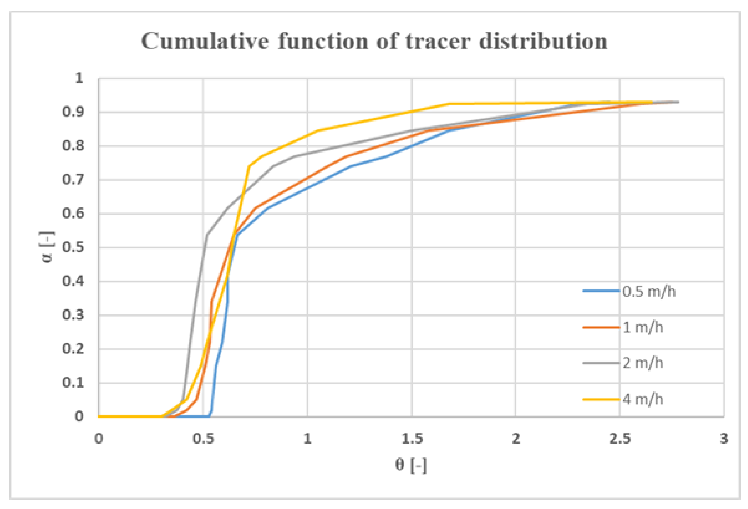
  • Based on a numerical tracer experiment, the tracer was already detectable at around 40% of the average residence time at the outlet, while more than 2.5 times the average residence time was required for 10% of the tracer to exit. The latter may indicate the presence of dead zones, while the former may indicate hydraulic short circuits.
  • The discrete phase model approximation provided acceptable results compared to the Eulerian multiphase model and the measurement results.
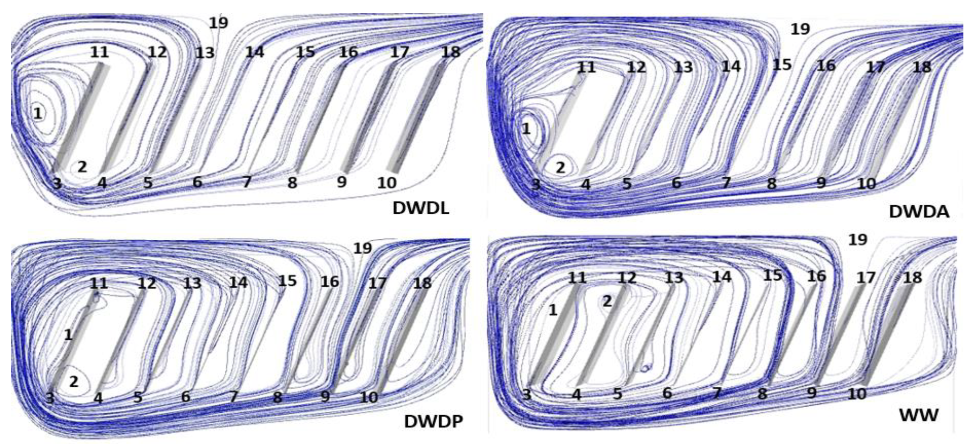
  • The consequence of the topological analysis was that two main flow zones formed in the lamella settler, with significant internal recirculation in the first zone. The boundary between the two zones varied with different loads, and the recirculation zone became more extensive with increasing loads.
  • Due to the recirculation eddies that formed in the reactor tanks, the actual hydraulic load could be much higher (from 1.5 to 4.5 times) than that in individual zones; therefore the design HLR, which referred to the entire tank, did not take into account the local flow pattern.
  • Depending on the load, the extent of the recirculation zone changed in a stepwise manner until the recirculation zone became so extensive that it included all the lamellae except the last one (from approximately 35 to 75% of the total volume).

Funding

This research received no external funding.

Institutional Review Board Statement

Not applicable.

Informed Consent Statement

Not applicable.

Data Availability Statement

The data are contained within the article.

Conflicts of Interest

The author declares no conflict of interest.

References

  1. Chai, L.; Li, Q.; Wang, Q.; Yan, X. Solid-liquid separation: An emerging issue in heavy metal wastewater treatment. Environ. Sci. Pollut. Res. 2018, 25, 17250–17267. [Google Scholar] [CrossRef]
  2. Mihopulos, J.; Hahn, H.H. Effectivity of Liquid-Solid Separation as a Function of Apparatus Characteristics and Wastewater Quality. In Chemical Water and Wastewater Treatment II; Klute, R., Hahn, H., Eds.; Springer: Berlin/Heidelberg, Germany, 1992. [Google Scholar] [CrossRef]
  3. Dufresne, M.; Vazquez, J.; Terfous, A.; Ghenaim, A.; Poulet, J.B. Experimental investigation and CFD modelling of flow, sedimentation, and solids separation in a combined sewer detention tank. Comput. Fluids 2009, 38, 1042–1049. [Google Scholar] [CrossRef]
  4. Spicer, P.T.; Pratsinis, S.E. Shear-induced flocculation: The evolution of floc structure and the shape of the size distribution at steady state. Water Res. 1996, 30, 1049–1056. [Google Scholar] [CrossRef]
  5. Chouippe, A.; Uhlmann, M. On the influence of forced homogeneous-isotropic turbulence on the settling and clustering of finite-size particles. Acta Mech. 2019, 230, 387–412. [Google Scholar] [CrossRef] [Green Version]
  6. Raeesh, M.; Devi, T.T.; Hirom, K. Recent Developments on Application of Different Turbulence and Multiphase Models in Sedimentation Tank Modeling—A Review. Water Air Soil Pollut. 2023, 234, 5. [Google Scholar] [CrossRef]
  7. Voermans, J.J.; Ghisalberti, M.; Ivey, G.N. The variation of flow and turbulence across the sediment–water interface. J. Fluid Mech. 2017, 824, 413–437. [Google Scholar] [CrossRef] [Green Version]
  8. Kreissl, S.; Pingen, G.; Maute, K. Topology optimization for unsteady flow. Int. J. Numer. Methods Eng. 2011, 87, 1229–1253. [Google Scholar] [CrossRef]
  9. Smith, B.T.; Halperin, J.; Darzins, A.; Davis, R.H. Enhanced sediment flow in inclined settlers via surface modification or applied vibration for harvesting microalgae. Algal Res. 2013, 2, 369–377. [Google Scholar] [CrossRef]
  10. Hurst, M.; Weber-Shirk, M.; Lion, L.W. Parameters affecting steady-state floc blanket performance. J. Water Supply: Res. Technol.—AQUA 2010, 59, 312–323. [Google Scholar] [CrossRef]
  11. Robescu, D.; Mandiş, C.; Robescu, D. Design lamellar secondary settling tank using numerical modeling. UPB Sci. Bull. Ser. D 2010, 72, 211–216. [Google Scholar]
  12. Vitasovic, Z.C.; Zhou, S.; McCorquodale, J.A.; Lingren, K. Secondary clarifier analysis using data from the Clarifier Research Technical Committee protocol. Water Environ. Res. 1997, 69, 999–1007. [Google Scholar] [CrossRef]
  13. Tarpagkou, R.; Pantokratoras, A. The influence of lamellar settler in sedimentation tanks for potable water treatment—A computational fluid dynamic study. Powder Technol. 2014, 268, 139–149. [Google Scholar] [CrossRef]
  14. Hirom, K.; Devi, T.T. Application of computational fluid dynamics in sedimentation tank design and its recent developments: A review. Water Air Soil. Pollut. 2022, 233, 22. [Google Scholar] [CrossRef]
  15. Haag, J.; Gentric, C.; Lemaitre, C.; Leclerc, J.P. Modelling of chemical reactors: From systemic approach to compartmental modelling. Int. J. Chem. React. Eng. 2018, 16, 1–22. [Google Scholar] [CrossRef]
  16. Fiedler, H.E. Coherent structures in turbulent flows. Prog. Aerosp. Sci. 1988, 25, 231–269. [Google Scholar] [CrossRef]
  17. Balachandar, S. Turbulence, coherent structures, dynamical systems and symmetry. AIAA J. 1998, 36, 496. [Google Scholar] [CrossRef]
  18. Gurka, R.; Liberzon, A.; Hetsroni, G. POD of vorticity fields: A method for spatial characterization of coherent structures. Int. J. Heat Fluid Flow 2006, 27, 416–423. [Google Scholar] [CrossRef]
  19. Epps, B. Review of vortex identification methods. In Proceedings of the 55th AIAA Aerospace Sciences Meeting, Grapevine, TX, USA, 9–13 January 2017. AIAA 2017-0989. [Google Scholar] [CrossRef]
  20. Calaf, M.; Hultmark, M.; Oldroyd, H.J.; Simeonov, V.; Parlange, M.B. Coherent structures and the k−1 spectral behaviour. Phys. Fluids 2013, 25, 125107. [Google Scholar] [CrossRef] [Green Version]
  21. Jiang, M.; Machiraju, R.; Thompson, D. Detection and visualization of vortices. In The Visualization Handbook; Elsevier: Amsterdam, The Netherlands, 2005; pp. 295–309. [Google Scholar]
  22. Deng, L.; Wang, Y.; Liu, Y.; Wang, F.; Li, S.; Liu, J. A CNN-based vortex identification method. J. Vis. 2019, 22, 65–78. [Google Scholar] [CrossRef]
  23. Hellsten, A. Some improvements in Menter’s k-omega SST turbulence model. In Proceedings of the 29th AIAA, Fluid Dynamics Conference, Albuquerque, NM, USA, 15–18 June 1998; p. 2554. [Google Scholar]
  24. Ferziger, J.H.; Peric, M. Computational Methods for Fluid Dynamics; Springer: Berlin/Heidelberg, Germany, 2001; ISBN 978-3-540-42074-3. [Google Scholar]
  25. Salamon, P.; Fernàndez-Garcia, D.; Gómez-Hernández, J.J. A review and numerical assessment of the random walk particle tracking method. J. Contam. Hydrol. 2006, 87, 277–305. [Google Scholar] [CrossRef]
  26. Karches, T.; Buzás, K. Investigation of residence time distribution and local mean age of fluid to determine dead-zones in Flow Field. Int. J. Comput. Methods Exp. Meas. 2013, 1, 132–141. [Google Scholar] [CrossRef]
  27. Rodrigues, A.E. Residence time distribution (RTD) revisited. Chem. Eng. Sci. 2021, 230, 116188. [Google Scholar] [CrossRef]
  28. Wang, Z.; Yang, Z.; Wang, X.; Yue, Q.; Xia, Z.; Xiao, H. Residence Time Distribution (RTD) Applications in Continuous Casting Tundish: A Review and New Perspectives. Metals 2022, 12, 1366. [Google Scholar] [CrossRef]
  29. Laramee, R.S.; Hauser, H.; Zhao, L.; Post, F.H. Topology-Based Flow Visualization, The State of the Art. In Topology-Based Methods in Visualization. Mathematics and Visualization; Hauser, H., Hagen, H., Theisel, H., Eds.; Springer: Berlin/Heidelberg, Germany, 2007. [Google Scholar] [CrossRef] [Green Version]
  30. Dao, N.T.M.; Liu, B.; Terashima, M.; Yasui, H. Computational fluid dynamics study on attainable flow rate in a lamella settler by increasing inclined plates. J. Water Environ. Technol. 2019, 17, 76–88. [Google Scholar] [CrossRef] [Green Version]
  31. Hirom, K.; Devi, T.T. Determining the Optimum Position and Size of Lamella Packet in an Industrial Wastewater Sedimentation Tank: A Computational Fluid Dynamics Study. Water Air Soil Pollut. 2022, 233, 261. [Google Scholar] [CrossRef]
  32. Jourdan, N.; Neveux, T.; Potier, O.; Kanniche, M.; Wicks, J.; Nopens, I.; Rehman, U.; Le Moullec, Y. Compartmental Modelling in chemical engineering: A critical review. Chem. Eng. Sci. 2019, 210, 115196. [Google Scholar] [CrossRef]
  33. Alvarado, A.; Vedantam, S.; Goethals, P.; Nopens, I. A compartmental model to describe hydraulics in a full-scale waste stabilization pond. Water Res. 2012, 46, 521–530. [Google Scholar] [CrossRef]
  34. Datta, A.; Bhunia, H.; Gupta, R. Residence time distribution studies on recycle reactor with recirculation. Int. J. Chem. React. Eng. 2021, 19, 1075–1088. [Google Scholar] [CrossRef]
  35. Pedersen, P.B.; von Ahnen, M.; Fernandes, P.; Naas, C.; Pedersen, L.F.; Dalsgaard, J. Particle surface area and bacterial activity in recirculating aquaculture systems. Aquac. Eng. 2017, 78, 18–23. [Google Scholar] [CrossRef]
  36. Aslam, A.; Khan, S.J.; Shahzad, H.M.A. Impact of sludge recirculation ratios on the performance of anaerobic membrane bioreactor for wastewater treatment. Bioresour. Technol. 2019, 288, 121473. [Google Scholar] [CrossRef]
  37. Schewe, G. Reynolds-number effects in flow around more-or-less bluff bodies. J. Wind. Eng. Ind. Aerodyn. 2001, 89, 1267–1289. [Google Scholar] [CrossRef]
  38. Wilson, T.E. Introduction and overview Water Environment Federation Clarifier Design, Manual of Practice No. FD-8. In WEFTEC; Water Environment Federation: Alexandria, VA, USA, 2005; pp. 4412–4416. [Google Scholar] [CrossRef]
  39. Luna, F.D.T.; Silva, A.G.; Fukumasu, N.K.; Bazan, O.; Gouveia, J.H.A.; Moraes, D., Jr.; Yanagihara, J.; Vianna, A.S., Jr. Fluid dynamics in continuous settler. Chem. Eng. J. 2019, 362, 712–720. [Google Scholar] [CrossRef]
Figure 1. Mesh and cell equiangle skewness distribution.
Symmetry 15 00864 g001
Figure 2. Model domain of the inclined plates.
Symmetry 15 00864 g002
Figure 3. Cumulative function of the tracer distribution at different hydraulic surface loads.
Symmetry 15 00864 g003
Figure 4. Streamlines and the most relevant critical points at various hydraulic loads (DWDL: dry weather diurnal hourly low, DWDA: dry weather diurnal average, DWDP: dry weather diurnal hourly peak, WW: wet weather instantaneous; the numbers refer to critical points).
Symmetry 15 00864 g004
Figure 5. Detailed and simplified compartmental model of the inclined settler at various loads (Q: incoming flow, r: recirculation rate, AI: first compartment settling area, n: number of recirculation cycles).
Symmetry 15 00864 g005
Figure 6. Zone 1 volume ratio in relation to the design HLR.
Symmetry 15 00864 g006
Table 1. Classification of critical points based on the eigenvalue of the velocity gradient tensor.
Name of the Critical PointReal and Imaginary Part of the Eigenvalue
Saddle point (S)Re1 < 0, Re2 > 0, Im = 0
Attracting node (AN)Re1 < 0, Re2 < 0, Im = 0
Repelling node (RN)Re1 > 0, Re2 > 0, Im = 0
Attracting focus (AF)Re1 < 0, Re2 < 0, Im < >0
Repelling focus (RF)Re1 > 0, Re2 > 0, Im < >0
Center (C)Re1 = 0, Re2 = 0, Im < >0
Table 2. Steady-state scenarios.
Scenario NameHydraulic Loading Rate [m/h]
Dry weather diurnal average (DWDA)1
Dry weather diurnal hourly peak (DWDP)2
Dry weather diurnal hourly low (DWDL)0.5
Wet weather instantaneous (WW4
Table 3. Particle separation efficiency.
Actual SimulationLiterature Data [30]Deviation
DWDL0.94no data
DWDA0.840.885%
DWDP0.60.658%
WW0.56no data
Table 4. Average velocities and turbulence-related parameters at the simulation domain at various hydraulic loads.
DWDLDWDADWDPWW
velocity magnitude (m/s)1.16 × 10−42.85 × 10−46.9 × 10−41.21 × 10−3
perpendicular velocity (m/s)6.52 × 10−89.47 × 10−81.38 × 10−71.88 × 10−7
turbulent kinetic energy (m2/s2)3.33 × 10−108.7 × 10−105.58 × 10−97.46 × 10−8
turbulent dissipation rate (m2/s3) 9.43 × 10−131.52 × 10−127.5 × 10−121.53 × 10⁻¹¹
turbulent viscosity (kg/ms)3.86 × 10−61.18 × 10−57.03 × 10−56.4 × 10−4
Table 5. Signs of the eigenvalues of the velocity gradient (Jacobian) matrix near the critical points.
12345678910111213141516171819
Re1----------+++++++++
Re2----------++++++++-
Im<>0<>000000000000000000
ClassAFAFANANANANANANANANRNRNRNRNRNRNRNRNS
Table 6. Hydraulic loading rates and their parameters in the different scenarios.
Design HLR
[m/h]
HLRZone 1
[m/h]
HLRZone 2
[m/h]
r
[-]
m
[-]
AI/A
[-]
DWDL0.51.330.750.291.450.33
DWDA11.662.250.381.50.56
DWDP22.707.140.431.470.72
WW45.1818.000.451.440.78
Disclaimer/Publisher’s Note: The statements, opinions and data contained in all publications are solely those of the individual author(s) and contributor(s) and not of MDPI and/or the editor(s). MDPI and/or the editor(s) disclaim responsibility for any injury to people or property resulting from any ideas, methods, instructions or products referred to in the content.

