Fathoming the Mandela Effect: Deploying Reinforcement Learning to Untangle the Multiverse

Abstract

Multiverse is a hypothetical idea that other universes can exist beyond our own. Various scientific theories have suggested scenarios such as the existence of bubble universes that constantly expand or string theory that attempts to merge gravity with other forces. Thus, a multiverse is a complex theoretical phenomenon that can best be conceived through computer simulation. Albeit within the multiverse, the causality of the Mandela effect is entirely possible. To examine the behavior of the multiverse as a representative ensemble, each universe as a specific ensemble element needs to be generated. Our universe generation is based on unique universes for two binary attributes of a population of $n=303$. The maximum possible universes this could produce within the multiverse is in the exponent of 182. To computationally confine the simulation to the scope of this study, the sample count of the multiverse is $n_{multiverse}=606$. Parameters representing the existence of each multiverse are implemented through the $\mu$ and $\sigma$ values of each universe’s attributes. By using a developed reinforcement learning algorithm, we generate a multiverse yielding various universes. The computer gains consciousness of the parameters that can represent the expanse of possibility to exist for multiple universes. Furthermore, for each universe, a heart attack prediction model is performed to understand the universe’s environment and behavior. We test the Mandela effect or déjà vu of each universe by comparing error test losses with the training size of order M. Our model can measure the behavior of environments in different regions referred to as specific ensemble elements. By explicitly exploiting the attributes of each universe, we can get a better idea of the possible outcomes for the creation of other specific ensemble elements, as seen in the multiverse space planes.

1. Introduction

Computer simulations offer the opportunity to model environments, their variables, and actors that exist in the occurring time plane. Each change in the parameters of the simulation model creates a unique simulated universe relying on an established classically computing concept. The implication that each of those simulated universes can occur simultaneously yields the idea of multiple parallel universes, a multiverse, or more accurately, a representative ensemble [1].

Most scientists believe that the multiverse is practically impossible to test because it is assumed that independent universes cannot interact. This also implies that the laws of nature in each of these universes must be different for them to be considered the same. To align our work with the standard statistical view on such problems, on some occasions, the term a specific ensemble element means universe, whereas a representative ensemble refers to a multiverse.

The multiverse has been flirted with as an idea in popular entertainment. From a computational standpoint, we can simulate the occurrence of a cascading, stacked, or nested multiverse by independently simulating the model of each specific ensemble element. Advances in parallel and distributed computing have allowed the aliasing of a representative ensemble during simulation runs, and recent advances in quantum computing have led to the development of methods to compute the representative ensemble by leveraging the mechanism of the specific ensemble element itself [2,3]. The aim of this research is to prove the implied representative ensemble using well-established theories that govern classical computing. Computing simulations created through parallel computing allow for the environment variables of each specific ensemble element to exist independently from other coexisting simulated universes. However, the simulation engine itself is unaware of the existence of each computed specific ensemble element as a parallel reality to another computer-specific ensemble element, treating each specific ensemble element as an independent element [4]. The concept of the multiverse and parallel reality can then explain the phenomenon known as the Mandela effect. The déjà vu or Mandela effect occurs when a large portion of the population mistakenly thinks that a certain event or memory happened. As a paranormal researcher, Broome [5] coined the term “collective false memory” after she learned that a large number of people at a gathering in 2010 shared an inaccurate memory of Mandela’s death in prison during the 1980s. Mandela was alive when the gathering occurred; he passed away in 2013.

A digital simulation of a representative ensemble allows scientists to create a complex theoretical framework that can be used to study the behavior of different specific ensemble elements. One of the most important factors to be considered when developing a multiverse is the creation of a specific ensemble element. For this purpose, we used a set of unique specific ensemble elements composed of two binary attributes. We assumed that the maximum number of specific ensemble elements that could be produced within the representative ensemble using the given set of parameters was 182. To ensure that the simulation was only focused on the scope of the study, the sample count for the representative ensemble was set at 606. The parameters used to represent the specific ensemble elements’ attributes were implemented using the $mu$ and $sigma$ values. The creation of multiple specific ensemble elements using the reinforcement learning (RL) algorithm allowed the computer to gain a deeper understanding of the possibilities of the existence of different specific ensemble elements. The concept of RL is becoming increasingly important in the development of artificial intelligence (AI) and the training of models that are based on machine learning (ML). We also performed a heart attack prediction model as a test of the déjà vu on each specific ensemble element. It took into account the training size of the order parameter and the error test losses.

In summary, this work makes the following contributions:

• Parallel Computing Simulation. We prove the existence of a representative ensemble using well-established theories of classical computing. Through parallel computing, the environment variables of different specific ensemble elements can exist independently of each other.
• AI/ML Algorithm Development. Through the use of RL, the computer simulation can create multiple specific ensemble elements with different dimensions. We developed an algorithm where an agent was trained to perform a specific task in an unfamiliar environment. The environment’s conditions and the rewards available for completing the task influenced the agent’s behavior. The training losses were computed by taking into account the predicted value of the false assumptions in the population’s specific ensemble element.
• Theory Testing. To test the Mandela effect, we generated a prediction model for a heart attack. According to the multiple universes theory, patients in each specific ensemble element will have a false memory of experiencing a heart attack. The effect will be magnified in a representative ensemble where people will believe that those who suffered a heart attack may not have experienced the same heart attack in the other specific ensemble elements.

To this end, this manuscript is structured as follows: Section 2 covers the literature review, including previous related work and background about the multiverse and the Mandela effect. Section 3 explains how we deploy the reinforcement learning algorithm to design the representative ensemble, what are data model parameters, and an overview of different types of RL algorithms. Next, Section 4 presents the simulation results that involve seed generation, heart attack prediction model, and fathoming the Mandela effect based on our model. In Section 5, we discuss our finding and give recommendations for future work. Finally, we reflect on our research and offer conclusions in Section 6.

2. Literature Review

The past few years have seen the emergence of physics-inspired computing, which has gained popularity and made advancements in various fields. However, there are many problems that remain unsolved. Some of these include the classification methodology, the gap between practice and theory, the selection of an appropriate algorithm, and parameter tuning. In this section, we dive into some previous research and basic fundamentals. Bostrom’s [1] foundational work on the simulation hypothesis implies the possibility of substrate independence, that is, consciousness being as capable as the computational power simulating it. Virk [6] uses the many worlds interpretation (MWI) concept through the lens of the developmental stages of simulated consciousness, which start at base reality and can progress through ten stages toward the simulation point of the simulation hypothesis constructed by a probabilistic determination that gets fractionally close to 100%.

In addition to the complexity involved in the simulation point progress, running simulations as stacked or nested, each complete with multiple universe constituent environments and variables, draws in huge computing power. This conforms to the parametric limitation described by Bostrom’s simulation hypothesis [1]. Limitations in computational power limit the levels at which a simulation can be run, possibly requiring termination of the simulation altogether should the nested simulations volumetrically expand beyond the computational power itself. This can limit the convergence of a multiverse [7].

Among the four types of multiverses Greene [8] theorizes, this study is focused on type 3—inflationary bubbles with fine-tuning, in alignment with the classical-computing domain. This specificity allows the measurement of multiple timelines to analyze simulated specific ensemble elements. Minkowski’s space-time diagram [9] laid the basis for measuring Einsteinian particle motion (variables in our construction) in space (universe). Successive advances in ways to measure the universe relative to the multiverse, such as the block universe snapshot and the delayed-choice experiment, have been built on the foundation of the space-time diagram.

The ongoing popularity of the multiverse has aroused great interest in theorizing and measuring parallel universes. The elemental concept of the multiverse that realities can be versatile, implying the possibility of multiple or parallel realities, can be traced back to Einstein’s theory of relativity [10]. The 1905 relativity theory paved the way for the general acceptance of symmetry as a valid theoretical basis. The existence of unnaturalness in different arenas, such as nuclear physics, cosmogenetics, and electroweak symmetry, indicates the possibility of a multiverse. The multiverse model can be described in a maximally symmetrical manner if the baryon asymmetry and zero vacuum energy are not encountered [11].

In addition to the infinity convergence [12], Bhattacharjee [13] notes bread-slice time and block theory, temporal monodromy, temporal exponentiality, and Mandela effect as additional ways to conceptualize the multiverse. Deutsch [14] calls the multiverse virtual reality, tracing its origins to the diagonal argument. Computational limits to simulating a multiverse have been overcome through the compilation of theories described by CantGoTu environments. At the sub-element level of such an environment of the multiverse, Turing positions the requirement of a universal computer that can calculate, simulate, and render multiple environments using computational logic [14].

In addition to considering the mathematical modeling and measurement of a multiverse, it is important to consider the various types of multiverses various researchers have categorically defined [3,15]. Tegmark [16] describes multiverses based on four types, progressing from Level 1 (an extension of our universe) to Level 4 (ultimate ensemble). Greene [8], in addition to his theorization of four types of multiverses, describes nine categorical types of multiverses: quilted, inflationary, brane, cyclic, landscape, quantum, holographic, simulated, and ultimate. Additional multiverse-type definitions have been described using twin-world models and cyclic theories.

The pursuit of modeling a multiverse offers researchers and data scientists the advantage of analyzing data that may have a variety of possibilities that are conceptually difficult to imagine but logically possible. Thus, simulating a multiverse provides optionality to the decision-making process in data influenced by the Mandela effect. However, as a natural constraint, the analysis of the multiverse only interacts with the analytical decision-making, data acquisition, and data cleaning processes. To resolve this limitation, Rijnhart et al. [17] propose the use of real data sets of varying environments of interest, each consisting of its own data acquisition method. Bell et al. [18] present a multiverse modeling and analysis technique with a Gaussian process surrogate for a type 4—higher dimension—multiverse and apply a Bayesian experimental design. Their model focuses on efficiency in the exploration of multiverses using ML. Wessel et al. [19] replicate memory suppression of the Mandela effect on real data sets by performing a multiverse analysis. Their simulation features a task developed as think/no-think (TNT), which compares binary levels of dissociative individual performance. By creating a parallel universe for their data analysis process, the researchers successfully tested the suppression effect on individual memory inhibition, thus proving the reduction of the Mandela effect of false shared memories in a large number of people.

2.1. Multiverse

The multiverse encourages the idea of altering retrocausality [20], dubbed by physicists as states of the past, present, and future. This is the materialistic model of the multiverse. However, measuring the representative ensemble through a delayed-choice experiment invalidates this model based on Wheeler’s theory of observation being the proof of a phenomenon. Wheeler’s theory also sheds light on Schrodinger’s cat (the disappearance of multiple realities upon observation). Therefore, the spatialization of time as multiple parallel retrocausalities can be more reasonably measured through the block universe snapshot, which is consistent with classical mechanics, as argued by Deutsch [14], and further supported by Virk [6].

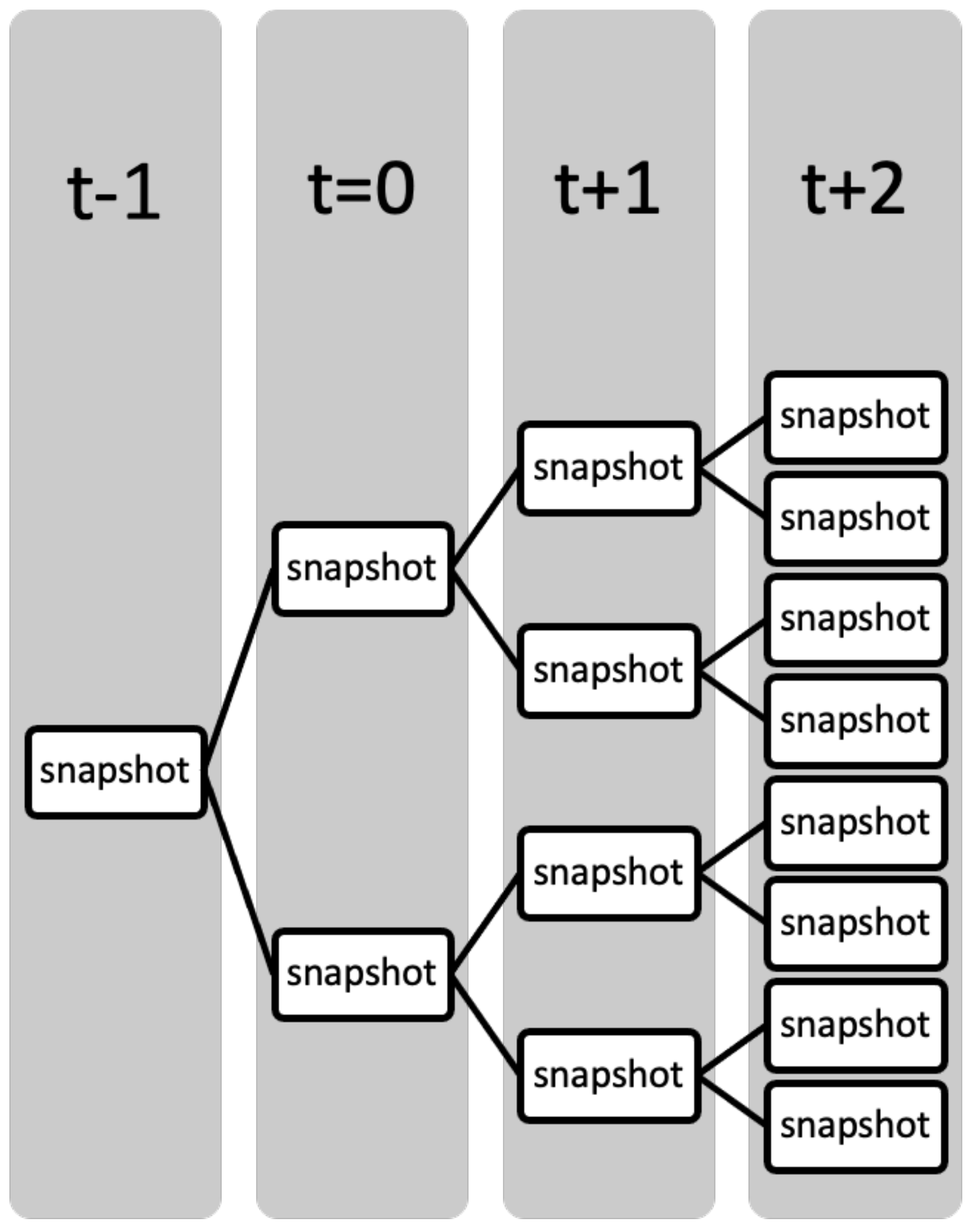
Based on block universe’s time spatialization, simulated universes can be saved in different states of time $\left(t\right)$ that store the environments, variables, and behaviors of each universe (Figure 1). Each state of t is a snapshot of the universe that can be traversed through the range $(-inf<t<inf)$ stored by the simulation or that can be limited by computational power. Although the example in the figure provides a minuscule snapshot to describe the idea, a multiverse requires that each causation of time has multiple snapshots of each independent universe, as Deutsch [14] indicates.

Super-snapshots are another way to describe a multitude of snapshots, where multiple versions of each snapshot universe exist in a given space. This parallelization is important for researchers to possess multiple reasonable options for any decision to be taken regarding any data. Analyzing this parallelization of super-snapshots allows for a representative ensemble analysis. As described earlier, a multiverse can be distinguished by its various types. A classic multiverse analysis is conducted by analyzing each snapshot in the super-snapshot multiverse to measure the simulation outcomes, ultimately affecting the decision [21].

Furthermore, the concept of the quantum landscape multiverse refers to the universe’s evolution from a wavefunction before inflation to a modern classical universe. It involves the entanglement of various branches of the wavefunction, which is a second source of correction for the universe’s gravitational potential. Rubio et al. [22] discuss the possible consequences of a multiverse theory based on the Majorana and Dirac quantized universe. Their approach unifies dark energy and gravity because Lagrangian’s equations of motion [23] are related to a relativistic particle [24].

2.2. Mandela Effect

In 2009, Fiona Broome created a website to share her thoughts on the Mandela effect. During a conference, she discussed the death of Nelson Mandela, who was the former president of South Africa. Mandela did not die in prison during the 1980s; he passed away in 2013. As she started talking to other people about her experiences, she realized that there were people like her. Some of them recalled seeing news coverage of Mandela’s death and a speech by his widow [5].

The Mandela effect, or déjà vu, is a phenomenon involving consistent false memories that emerged with the growth of the internet. The increasingly popular hypothesis that our reality is a simulated augmentation suggests that the past, present, and future exist simultaneously in parallel universes. The reason for a serious investigation of such a possibility stems from perceptions of observed reality shared by millions of people who may be geographically far apart [25].

Although the Mandela effect and the déjà vu phenomenon are similar, they have slightly different definitions. The former involves several individuals, while the latter involves only one person. According to Dr. Khoury, déj vu is caused by a miscommunication between the parts of the brain that play a role in remembering and familiarity, which result in false memory, but the Mandela effect is more challenging to explain because it involves more people.

Inhibition theory underlines the occurrence of replicated memory signatures that provide novel cues to the existence of a multiverse. The web of connectivity constructs a consciousness existing in the dimensionality of time, allowing the past, present, and future to be changed and creating a parallel universe [26].

Simulating reality as multiple augmented replications stretch the possibilities of classical physics. Although quantum physics is being explored as a domain, studies suggest that it is not outside the realm of possibility for classical physics to observe the inhibition of memories in parallel environments. The perception of the spatial transformation of space-time may be outside the realm of human psychological imagination. However, the capable limits of computational power have demonstrated that simulations can yield multiple copies of data based on the logical confines of an environment’s possible implications [27].

In addition to calculating the various levels of simulated specific ensemble elements, achieving consistency of each simulation to maintain efficient computation for the entire span of retrocausality is vital to the sustainability of the Mandela effect and, thus, by extension, the multiverse [28]. Computational or commutable lag or delays in the simulation reduce the flow of environmental states between time, creating gaps in the data of the space-time diagram based on the simulation hypothesis.

3. Reinforcement Learning Deployment

3.1. Designing the Multiverse

The question of what a good model should be for the universe is dependent on not only the properties we want to model but also the theoretical framework we have chosen. For instance, if we want to describe the specific ensemble element using a massive wave function, it might be natural to do so by developing it in real time. At the same time, if we want to model the universe using general relativity, it might be possible to create a more natural model by combining the distribution of mass-energy with a pseudo-Riemannian manifold [29].

Proposals have been made to design the multiverse through consciousness based on tje well-established theories of Deutsch, Greene, and Virk [6,8,14]. By using real-world data to train the RL algorithm, simulations can be created in parallel through the statistical probability of data sets capable of characterizing various states for a variety of universes.

The representative ensemble design proposed in this study was based on type 3—inflationary bubbles [30] with fine-tuning. In this type of multiverse, multiple universes are created from a single point of origin that seeds amplified fluctuations of possibilities into each universe. The environment generated in each universe has a probabilistic determinant [31] shaping its configuration to modify variable values that create distinct copies identified by a unique seed label.

In RL, an agent can interact with its environment for a (discrete) time step before it is reset and repeated in subsequent episodes. The goal of the exercise is to maximize the agent’s performance. Thus, each seed is populated with its own environment, variables, and behavior. Seed generation is performed using Monte Carlo simulation for random number generation of each of the parametric variables defined in the point of origin [32]. To define the Monte Carlo design for each specific ensemble element, there needs to be a time axis for the spatial domain parameters of the environment. The time axis is considered an integral of function space:

$$Int={\int }_a^{b}f\left(x\right)dx$$

(1)

In the space domain, X is assumed to be a uniformly distributed random variable of closed interval $[a,b]$. Based on these variables, Monte Carlo will generate an estimate of the expected seed value based on n samples as follows:

$$See{d}_n=\frac{1}{n}\sum _i^{n}f\left(X_i\right)$$

(2)

where the expected value of the uniformly distributed random variable X in the closed interval of the integral is formulated as follows:

$$Int=(b-a)E\left[f\right(X\left)\right]$$

(3)

Based on (2) and (3), the equation for the approximate value of the integral in (1) becomes:

$$I_n=(b-a)\frac{1}{n}\sum _i^{n}f\left(X_i\right)$$

(4)

Another type of computation that is commonly used in the design of a representative ensemble is the time average. These are the average values that are taken for the various realizations of the process. Whereas the ensemble averages are usually taken into account when making a realization of the stochastic process, a time averaging is taken for a specific realization. Although the space average and time average may seem to be different, if the transformations are invariant and ergodic, then the former is equal to the latter in almost all cases. As the number of samples $n\to \infty$ is increased closer to infinity, the sample average of the seed $See{d}_n$ will converge to $E\left[f\right(X\left)\right]$, producing (1).

The Monte Carlo process creates the likelihood of similarities among specific ensemble elements:

• Multiple specific ensemble elements have identical parameters;
• No two specific ensemble elements have identical parameters;
• Multiple specific ensemble elements have several identical parameters, but not all parameters are identical.

The estimation of uniformity is performed through a Gaussian normal distribution. The yielded data become Poisson data. Considering the central limit theorem in the Monte Carlo estimation of the expected value of samples as they reach closer to infinity, the yielded seed generation will abide by a normal distribution of samples as follows:

$$\sqrt{n}(See{d}_n-\mu )\to N(0,{\sigma }^2)$$

(5)

In this normal distribution $N(0,{\sigma }^2)$,

$$\begin{array}{c}\hfill \mu -E\left[f\right(X\left)\right]\\ \hfill {\sigma }^2-Var\left(X\right)\end{array}$$

(6)

The Poisson data can be manipulated to alter the parameters of each specific ensemble element, rejecting or modifying the parameters as they see fit. By altering the values of mean $\mu$ and the square of variance ${\sigma }^2$ through Monte Carlo, Laplace approximation, or Bayesian probability, we will receive a cumulative density function (CDF) that we can use to compare the sample density of each specific ensemble element seed in the representative ensemble:

$$CD{F}_{seed}=\frac{1}{2}\left[1+erf(\frac{(x-\mu )}{\left(\sigma \sqrt{2}\right)})\right]$$

(7)

The error estimation for the Monte Carlo estimation of the expected seed value can be calculated by subtracting the difference of the seed estimated value from the mean $err\to See{d}_n-\mu$. For a random variable Z, the error estimation can be rewritten as follows:

$$err\to \frac{1}{\sqrt{n}}Z$$

(8)

3.2. Data Model Parameters

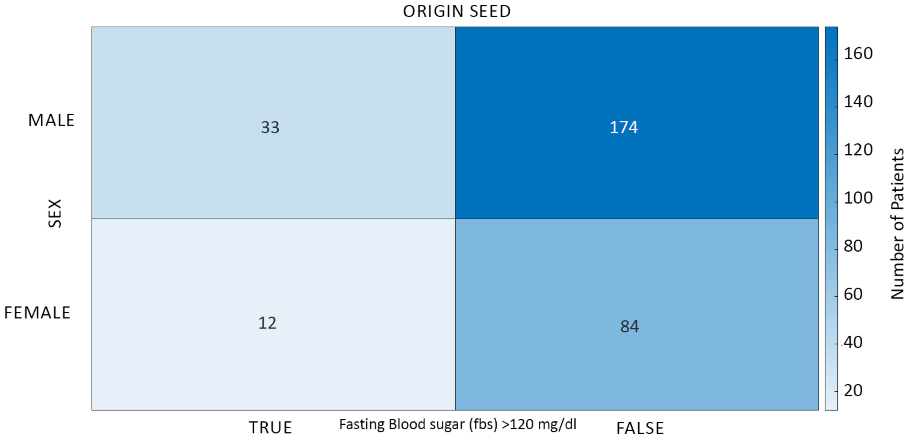
We used a real-life dataset of 303 randomly sampled patients measured by the health conditions of their heart as the point of origin for comparing all other generated specific ensemble element seeds. The parameters of the data model were extracted from a dataset containing a total of 13 measured attributes of each patient. Two data attributes were chosen to represent a model that predicted the likelihood of a heart attack in patients based on their health conditions: fasting blood sugar (fbs) and patient sex. These two attributes were chosen based on the closest medical correlation that leads to a heart attack. For our heart attack prediction model, a binary value represented each of the two attributes.

$$\begin{array}{c}\hfill fbs\left\{\begin{array}{cc}1;\hfill & >120\frac{\mathrm{mg}}{\mathrm{dl}}\hfill \\ 0;\hfill & <120\frac{\mathrm{mg}}{\mathrm{dl}}\hfill \end{array}\right.\\ \hfill sex\left\{\begin{array}{cc}1;\hfill & \mathrm{male}\hfill \\ 0;\hfill & \mathrm{female}\hfill \end{array}\right.\end{array}$$

(9)

These two attributes were stored in a data sheet labeled as X. Accompanying them were two attributes stored in another data sheet labeled as t, which contained true binary data of actual heart attacks each patient experienced in the data.

These data were considered the origin data that served as the fundamental parameters to create specific ensemble elements in the representative ensemble. Mapping of the data model as specific ensemble elements in the representative ensemble was based on the specific ensemble element parameters of fbs and sex. Each parameter was measured by its mean ($\mu$) and standard deviation ($\sigma$) and mapped on a 2D plane.

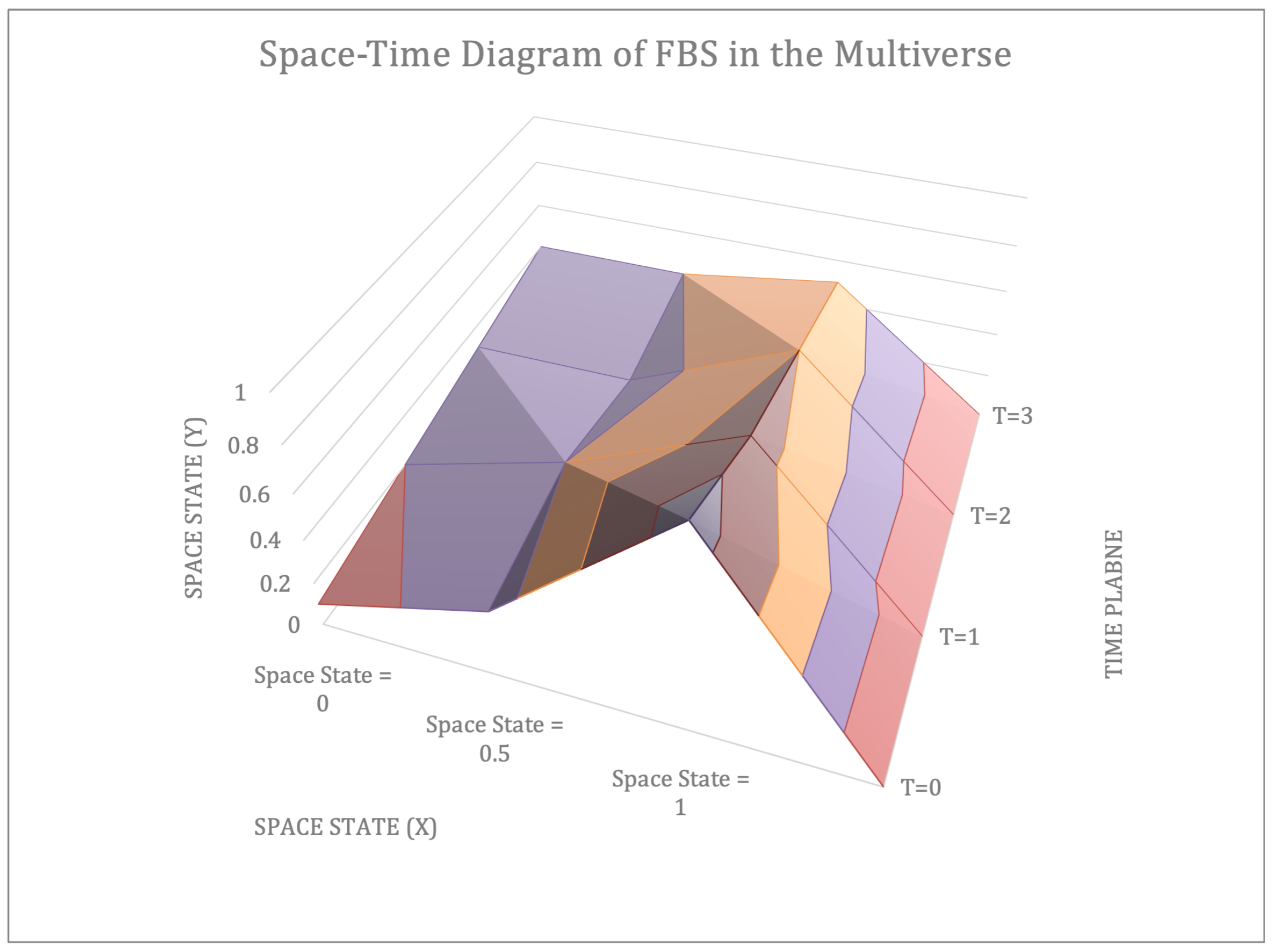
A space state is a representation of a system’s possible configurations. It can be used in the analysis of systems in the fields of game theory and artificial intelligence. For instance, a space state can be used for solving the shortest path problem known as Vacuum World. It can also be used for describing the valid state of the eight queens puzzle. The space state at the $t=0$ time state of the representative ensemble. The functioning representative ensemble has space states of each specific ensemble element that vary with time states. Therefore, the values of $\mu$ and $\sigma$ vary at each time state based on their environment, showing that the specific ensemble element is not flat. Figure 2 shows the space-time plane for measuring the data model in the representative ensemble. This figure is an illustrated example to help visualize the multiverse. The X-Y plane of the space state represents the standard deviation and mean with no specific data points. In the simulation, we used time plane T = 0 for illustrations.

3.3. Reinforcement Learning

Computers can be taught to learn in complex environments that are entirely new and dynamically changing. Such a learning methodology requires a direction specified by a goal or a reward. It influences the computer’s decision-making process for following the activity sequence that provides the most rewards without any external intervention or involvement of human intelligence. Thus, the computer performs a series of activities to train itself by evaluating the outcomes it is able to generate based on the reward. This learning process is described as RL.

In the meta of RL, an agent is defined as having the exclusive goal of being trained to perform and accomplish tasks in unfamiliar environments. Behavioral influence on the agent’s activities is managed by observation of the environment and the possible reward(s) for completing assigned tasks.

Further, an agent’s behavior fundamentally comprises two elements: a learning algorithm and policy. Both elements have an interdependent relationship. At the elemental level, it is the policy that specifies the actions an agent can or cannot undertake in a given environment. Policy is commonly established through observation, which can be altered to fit the environment the agent is operating in. As a result, the learning algorithm depends on a policy that is based on a relationship of mutual exchange—the variables of the policy are updated on the basis of activities and observations gathered by the agent. Ultimately, the learning algorithm must determine a pathway by formulating a policy that results in the maximum possible outcome or reward an agent can achieve in the environment through its actions.

Thus, as the name suggests, RL is a computational process where the computer (defined by one or more agents) interacts with the environment by iteratively improving its activity without any external human intervention. Driving the computational process is a workflow scheme. At the fundamental level, RL follows its underlying workflow (Figure 3), training agents to subscribe to behaviors.

RL eliminates the need for human involvement, allowing the computational technique’s implementation across a wide scope. RL’s primary uses consist of automated robots, vehicles, and characters in computer games as well as more recent consumer applications. RL can be used for activities as simple as parking a self-driving car or suggesting movies to a user based on their viewing habits. Critical to RL are the precursor data acquired through sensory instruments, data-capturing applications, or both. Agents alter their behavior based on repeated interactions with the environment and acquired data. Effective RL systems take into consideration environmental noises and other edge-case deviations, preventing any erratic action that may not match the ordinary purpose or goal the agent must act upon.

Another vital attribute of reliable RL systems and their agents is the minimization of the repetition required as a part of learning. This attribute is vital because although it can lead to agents learning, it has not attained the performance or the corresponding behavior for actions that yield established rewards. Therefore, the trial-and-error process incurs costs to the overall system. These costs can sometimes include things such as accidentally smashing a self-driving car into an unrecognized object (a pedestrian or an object that can damage or destroy the car itself). Many similar analogies exist in their respective domains.

The iterative nature of the learning process also involves memorizing decision states and policies so as to decide the future adoption of policies through comparison with past policies. Memorization and comparative decision-making systems increase the RL process’s reliability and efficiency. Such a feature is important because retraining agents must not be a costly process. Underlying parameters that require updates for agent(s) behavior are as follows: the environment’s dynamics, the configuration of the learning algorithm, the training settings, the evaluation of policy and reward value, the identification of the signals for reward, and the identification of the signals of observation as well as activities.

3.3.1. Types of Algorithms

Techniques to implement RL are characterized by its algorithms. The various algorithms that exist distinguish themselves based on their strategy for optimizing or maximizing one or more of the RL workflows. In the context of this study, these algorithms are described by their strategy, utility, and trade-offs. This allows for a comparative evaluation of the proposed algorithm that can help formulate the multiverse and Mandela effect. This study involves using MATLAB 2021 to estimate, model, design, and train RL agents for the representative ensemble.

Deep Q-Network (DQN). This RL algorithm has a value-based agent strategy. Agent(s) are trained at each time step to update the properties of the critic to estimate future rewards. DQN agents are trained with a specific behavior that conditions them to use a circular experience buffer to memorize prior experiences and perform an exploration of the environment. During environment exploration, agent(s) explore their action space using one of two methods. Either agent(s) choose an activity randomly, governed by a probabilistic nature, or agent(s) are driven by reward as defined by a value function. The choice of agent behavior occurs at each interval of control. A custom discrete environment is chosen for the DQN agent based on the binary value range interval of the data model parameters. Computations can be assigned to either the CPU or GPU at the time of configuring the environment [33]. The observation specifications take place in the time domain with dimension $\left[41\right]$, whereas the action specifications take place in the discrete domain with dimension $\left[11\right]$. The agent sampling time is set to 1, whereas the critic learning rate is set to $0.01$. Agent exploration during training is set to an initial epsilon of 1 for epsilon greedy exploration that decays at a rate of $0.005$ to an epsilon minimum of $0.01$ over 1000 steps. Agent training is limited to a maximum of 500 episodes and upon reaching the value of 500 average steps. The length of the maximum episode is set to 500, whereas the average window length is defined by the value 5.

Deep Deterministic Policy Gradient (DDPG). Agents of the DDPG algorithm focus their strategy on an optimal policy search targeting the maximum total long-term rewards that can be accumulated. At the time of training, the agents of this algorithm update the properties of the actor as well as the critic, in contrast to the DQN algorithm, which updates the properties of only the critic at each episodic learning. However, the agent’s behavior of memorizing prior experiences is similar to the agent’s behavior in the DQN. Another distinguishing feature of this algorithm is that it uses a stochastic noise model to interrupt the choice of action by the agent(s) for the defined policy. The DDPG algorithm retains several of the dimensional properties that configure agents of the DQN algorithm. These include the length of episodes, training steps, decay, dimensionality, and reward. The distinguishing features of the setup lie in the creation stages of the critic and actor, which involve defining the actions for the rewards based on observations [34].

Twin-Delayed Deep Deterministic Policy Gradient (TD3). This RL algorithm is another type of DDPG algorithm. Similar to DDPG, TD3 focuses on the exploration of the policy that provides the maximum long-term reward. TD3 distinguishes itself by reducing suboptimal policies chosen as a result of overestimating the value functions that DDPG agents perform. This algorithm improves upon that shortcoming by learning not one but two Q-value functions as well as by incorporating the minimum value function estimate at the time of updating its policies. As a result, agents of this algorithm are less frequently targeted compared to Q-functions. All other characteristics of the TD3 are fundamentally the same as those of DDPG. For this reason, the configuration of TD3 is similar to that of DDPG, with the only exception being the specification of the noise value of the target action that agents must perform to make actions less exploitable by policies [35].

Actor–Critic Method (A2C, A3C). As the name suggests, agents of the actor–critic method implement algorithms that are focused on the actor–critic strategy. This algorithm influences its agents in a discrete or continuous action space to directly optimize the policy for the actor followed by implementing a critic for reward estimation. This characteristic defines the goal that drives A2C or A3C agents. In contrast to previous algorithm strategies, the configuration of the A2C/A3C algorithm is set up such that agents of the actor–critic algorithm frequently interact with their environment, estimating the probability of the action that needs to be taken. This is followed by a probabilistic random selection of actions and then an update to the properties of the actor and critic [33].

Proximal Policy Optimization (PPO). In this algorithm, the strategy is to switch between two performance steps: (a) use the stochastic gradient descent to improve a segment of the objective function and (b) sample the data during interaction with the environment. This algorithm is a rather simpler version of the Trust Region Policy Optimization (TRPO) algorithm. Here, the segment, which is better defined as a clipped surrogate, limits the policy size changed at each step, improving the stability of the algorithm’s performance. The configuration of the PPO agents during training is similar in some ways to the A2C/A3C algorithm. Before updating the properties of the actor and critic, the agents frequently interact with the environment. There is also a random selection of actions in accordance with an estimated statistical probability in the action space [36].

Soft Actor–Critic (SAC). This is another algorithm that focuses on estimating and maximizing the long-term reward. The SAC also measures policy entropy, which refers to uncertainty in a policy. The greater the uncertainty, the higher the capability this algorithm has to explore the policy and environment. The result of this strategy is that SAC agents are able to achieve two objectives simultaneously: accumulate the maximum reward possible and balance the amount of exploration performed in the environment. Training of SAC agents involves a combination of features described in the DQN, DDPG, and actor–critic algorithms. Where the properties of actors and critics are routinely updated at the time of learning, prior values are memorized, and agents randomly choose actions based on a probabilistic model. The only distinguishing features here are that an entropy weight is updated as a part of the update routine. This is important for the algorithm because the measured entropy balances the reward and policy [37].

Q-Learning. This is one of the more commonly used and simpler algorithms in the RL space. Agents of the Q-Learning algorithm focus their strategy on the value of future rewards. Critics are trained to estimate returns from their observations of the environment and then choose actions that lead to the greatest returns. Much like the DQN agents described earlier, Q-learning agents explore their action space by implementing an epsilon-greedy exploration strategy. The choice of action is probabilistic and driven by the estimation of future rewards [38].

State-Action-Reward-State-Action (SARSA). SARSA is highly similar to the Q-learning algorithm in that it focuses its strategy on the value of future rewards. The only distinguishing feature is that the training of critics follows a procedural SARSA sequence to estimate returns from the critics’ observation of the environment, and then SARSA agents choose actions that lead to the greatest returns. Similar to Q-learning and DQN, SARSA agents explore their action space by implementing an epsilon-greedy exploration strategy. The action that has the greatest value is randomly chosen and driven by the estimation of future rewards [39].

Trust Region Policy Optimization (TRPO). In comparison to the PPO algorithm, this algorithm has a higher computational demand for training and simulation. However, the capability of the TRPO is more reliable in environments where its dynamics have low dimensionality in observation and are deterministic. Many features and configurations of TRPO are similar to those of PPO. The only distinguishing features are that TRPO switches between the sampled data from the environment and solve a constrained optimization problem before updating the policy parameters [40].

In the setup, the constraint encountered during optimization for the problem-solving uses KL-divergence. This helps the TRPO algorithm avoid performance compromises.

3.3.2. Designing the Mandela Effect

The Mandela effect suggests that patients in each specific ensemble element will carry a false memory of heart attacks experienced by other people in their specific ensemble element. This phenomenon will be magnified in the representative ensemble, where patients will believe that other patients bearing specific parameters of health conditions have suffered a heart attack. This may not be true in their specific ensemble element, but it may be true in another element within the representative ensemble.

Patients will be modeled as agents carrying beliefs in their own unique specific ensemble element. This is characterized by the measurement of training error losses of the prediction model. The heart attack prediction model in each specific ensemble element predicts the number of people who may suffer from cardiac arrest. This prediction model will create beliefs in the population. The false positive heart attacks reported by the trained model can then explain the Mandela effect. While the self-reported AI agent of false data points can act like a déjà vu effect.

The resulting prediction training losses will indicate the index value of false assumptions the population will have in its specific ensemble element (Algorithm 1).

Algorithm 1 Multiverse as Representative Ensemble Simulation Model

Require: For consciousness of the specific ensemble element, the algorithm detects the boundary conditions of the data set. Because we have two data points (fbs and sex), dimensions for each data point will exist as $D_{m,n}$ where D represents the data points fbs and sex Ensure: The boundary conditions are stored in the variables fbs = $[fb{s}_{ll},fb{s}_{ul}]$ and sex = $[se{x}_{ll},se{x}_{ul}]$ Calculate the $\mu$ (mean) and $\sigma$ (standard deviation) of the original data set to identify the origin value of the specific ensemble element. These values become fbs = $[\mu ,\sigma ]$ and sex = $[\mu ,\sigma ]$ and can be plotted on a Cartesian 2D plane Create the environment for the RL agents to populate the representative ensemble with multiple specific ensemble elements. The number of unique universes can be quantified by a smaller number while total number of specific ensemble elements $=n:S_n$ do     Generate a random value of fbs = $[\mu ,\sigma ]$ and sex = $[\mu ,\sigma ]$     Define a reward value for the agent to check and remove any duplicate values of $[\mu ,\sigma ]$ for each $D_{m,n}$      if $(D_{m,n}>1)$  then         total number of specific ensemble elements = total number of specific ensemble elements $-D_{m,n}$         Set $n=$ total number of specific ensemble elements      end if end while Create a data set of 303 array positions for each $D_{m,n}$ coordinate value while total number of specific ensemble elements $=1:S_n$ do      while total population $=1:Populatio{n}_n$ do         Define a reward value for the agent to randomly populate Matrix $M_{i,j}.(i=303,j=1)$ based on value of fbs = $[\mu ,\sigma ]$ and sex = $[\mu ,\sigma ]$      end while end while Measure each data set containing both data points for total number of specific ensemble elements

The computational complexity of this algorithm can be computed considering the first while loop with the condition if statement gives $\mathcal{O}\left(n^2\right)$, then the second set of while nested loops have the complexity of $\mathcal{O}\left(n^2\right)$, which means the total arithmetic complexity is $\mathcal{O}\left(max(n^2,n^2)\right)$, equal to $\mathcal{O}\left(n^2\right)$ where the performance is affected by the square of the input elements.

4. Simulation Results

4.1. Representative Ensemble Seed Generation

Representative ensemble parameters consisting of two binary value attributes (fbs and sex) from the data model yielded a total of $2.65$ possible unique seeds in the representative ensemble. The theoretical model of a representative ensemble allows it to possess multiple copies of each seed’s parameters to an infinitesimal amount. The number of unique seeds generated $\left(See{d}_n\right)$ in this study was sampled to 606 specific ensemble elements in the representative ensemble, $n=606$.

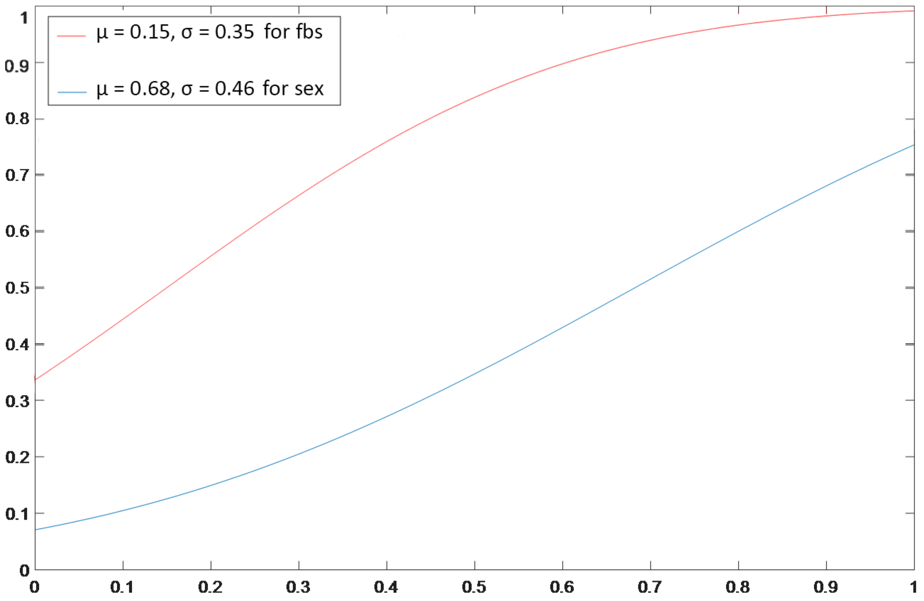
Figure 4 shows the distribution of two attributes characterizing the parameters of the origin seed of a specific ensemble element in the space plane at $t=0$. Figure 5 shows the distribution of the attributes.

Much like the origin seed in Figure 4 depicting the composition of 303 patients, each specific ensemble element in a representative ensemble has its own distribution based on the values of mean and standard deviation. Figure 5 depicts a Monte Carlo probability model that was performed without any RL.

Therefore, the representative ensemble algorithmic function became the following:

$n_{ensemble}=$

$$\begin{array}{c}\hfill \left(\left[\begin{array}{c}parameterLowerLimit\\ parameterUpperLimit\end{array}\right],populationSize,n_{element}\right)\\ \hfill ;\mu ,\sigma \end{array}$$

(10)

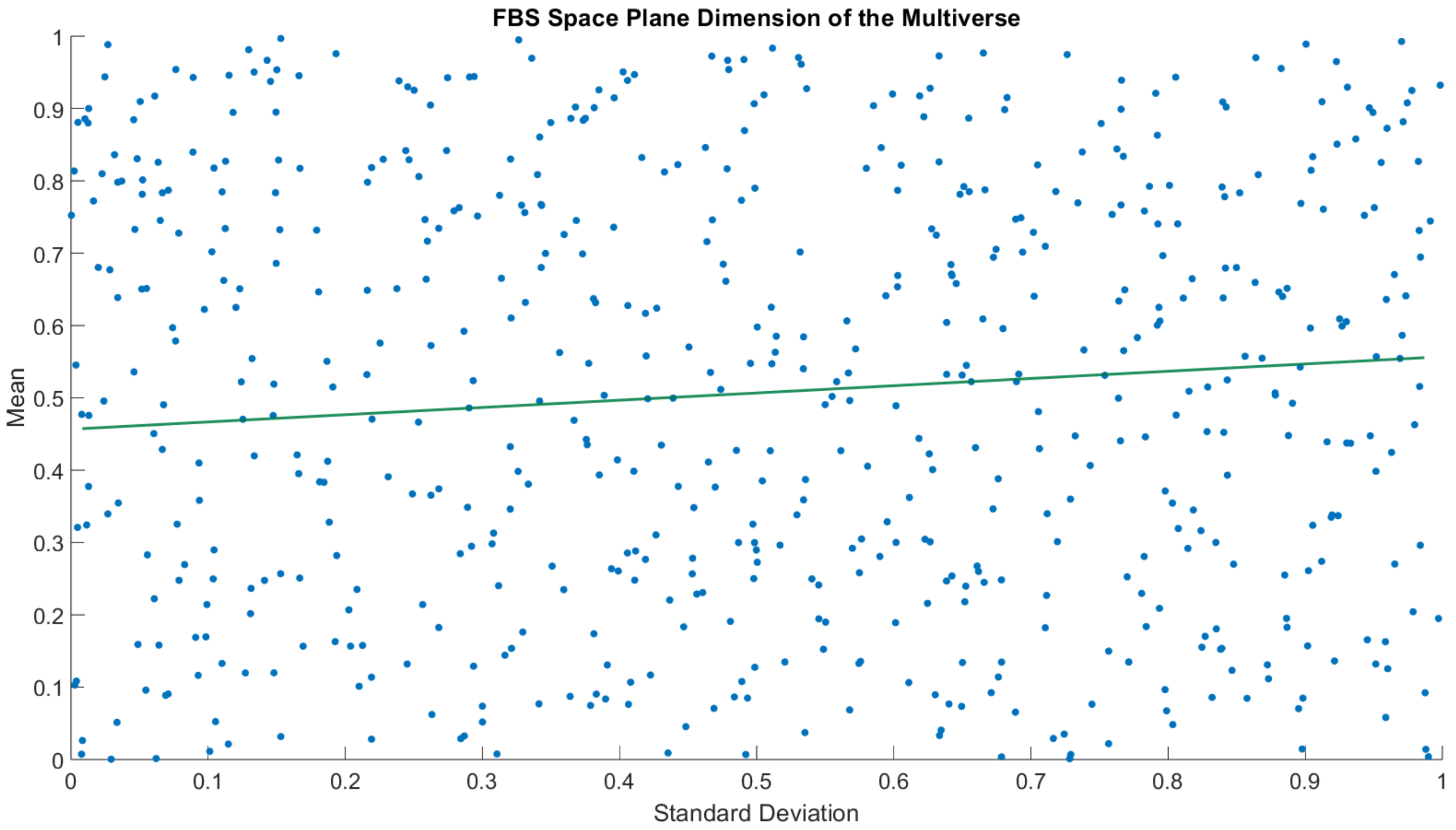
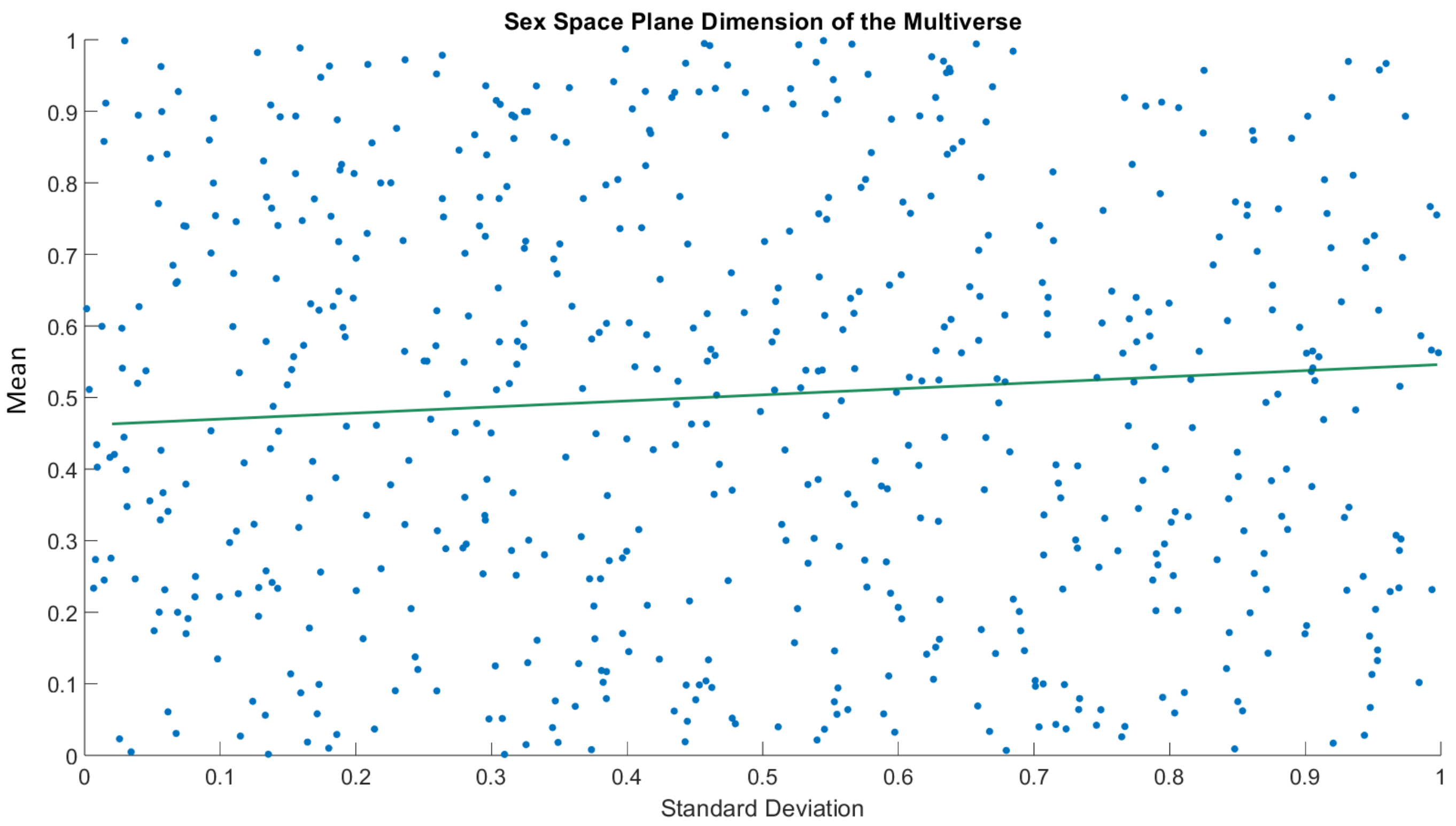
The space plane visualization of a clipped segment of representative ensemble generation can be seen in Figure 6 and Figure 7. Each point represents a specific ensemble element. It is important to note that both Figure 6 and Figure 7 represent two slices of the same representative ensemble at time $t=0$. This slicing was performed to render the parameters of each specific ensemble element in a two-dimensional plane. The 0–1 boundaries are the mathematical limits of the binary data shown in Equation (9). If the data were to be of any other number range, it would only increase the computational requirements for the simulation. Figure 6 and Figure 7 are snapshots of the simulated results X-Y at time interval $t=0$ of 606 ensemble elements, i.e., 606 points. Each point of the ensemble has 303 patients split by fbs and sex. The randsample sets up the environment to choose the value of mean and standard deviation between 0 and 1 differentiated by 3 decimal values, 0.0001. No two values are duplicates, which occurs frequently, as our model was built to avoid duplicating from happening.

4.2. Heart Attack Prediction Model in the Multiverse

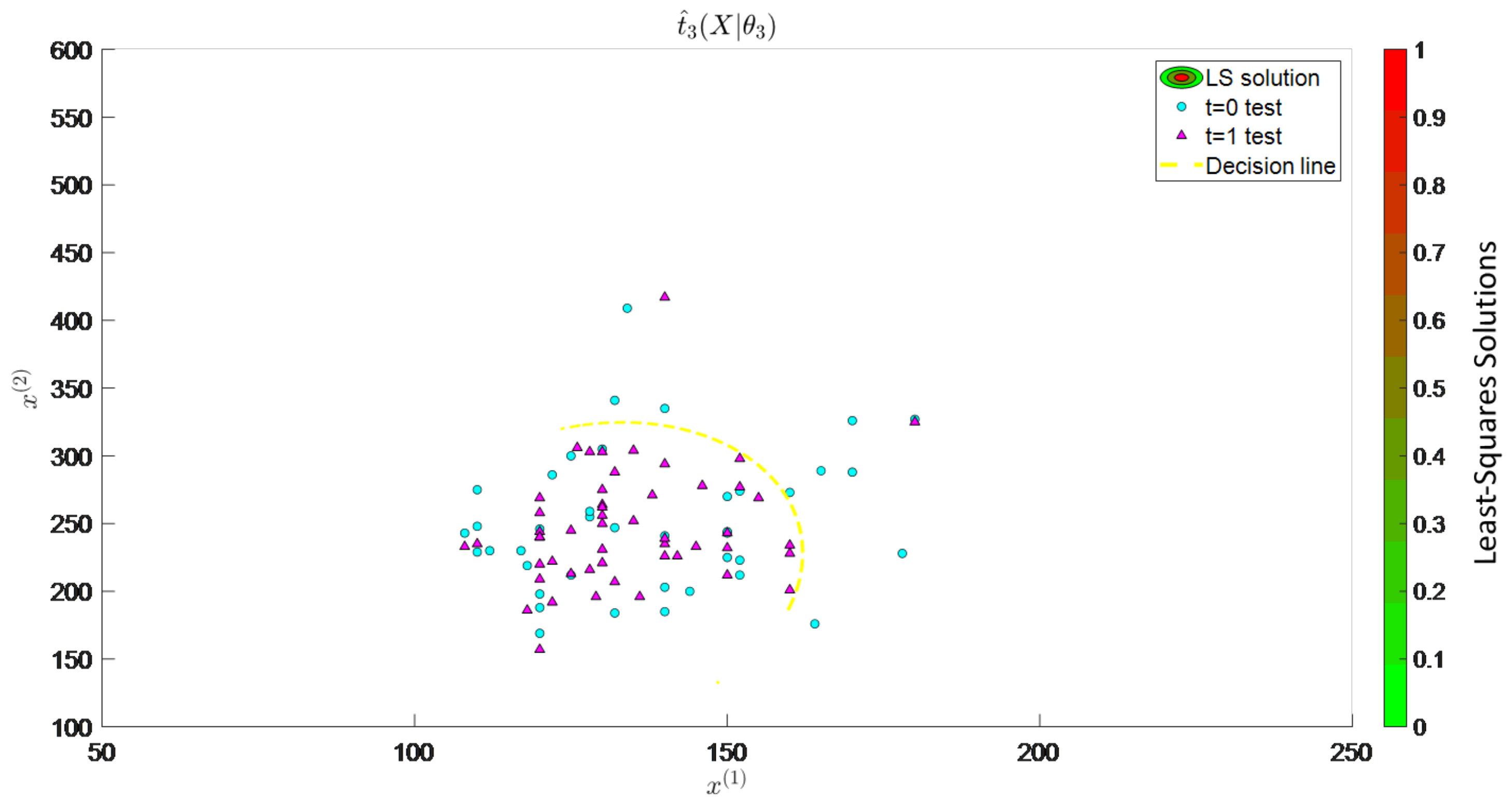
The heart attack prediction model was simulated for each specific ensemble element of the representative ensemble. Figure 8 shows the probability of patients in the origin seed-specific ensemble element at time $t=0$ who can experience cardiac arrest. These data were consistent with the distribution of attributes presented in Figure 5. Additional specific ensemble elements showed the prediction model based on their own parameter distribution, as seen in the representative ensemble space planes. Extending this concept to multiverse systems with cyclic individual-specific ensemble elements allows us to predict either increasing or decreasing entropy. A cyclic model is a type of cosmological model that indicates that the specific ensemble element follows an indefinite, infinite cycle, or self-sustaining cycles. According to the cyclic universe theory, the specific ensemble element experiences continuous cooling and expansion throughout its evolution. It starts with a Big Bang before going through a series of cycles, culminating in a “big crunch”. The time is considered an integral of function space, as shown in Equation (1).

Data are often cyclical; for instance, time is a rich example. It is a collection of features that are naturally related to cycles. We are trying to learn how to inform our machine-learning model about the nature of a feature in a dataset. Let us say we want to understand the 24-h time series. It could be connected to fbs or sex. However, we want to convey the idea of its cyclical nature. To learn how to convey the idea of time’s cyclical nature, we will first create fake time periods. We will only be looking at the time’s appearance on certain periods, such as 24-h clocks. The seconds past midnight do not exhibit closeness between the data that cross the “split”. With just the “fbs”, there is nothing to break symmetry across the entire period. However, we need two dimensions to create a cyclical feature, which is why we used “sex”. A feature with an out-of-phase component can also break the symmetry. By combining the two features, all time can be distinguished from one another. The time series’ cyclical nature can be observed in our RL model by feeding the fbs and sex features into it.

There are multiple ways to generate a representative ensemble; the most appropriate for this study is the cyclic time model. Essentially this method is an iteration space at each time plane, i.e., x-y points at each interval of time $t=0,t=1,t=2$, and so on.

Thus, applying a cyclic time model, we could see this prediction model change at different intervals of time for each specific ensemble element of the representative ensemble. In the simulation of each specific ensemble element, only the attributes of fbs changed, whereas sex remained the same for each population. This was performed to model the behavior of changes to the fbs levels of each patient in the population. Therefore, the changing values of mean and standard deviation of each fbs and sex value represented the environment of each specific ensemble element.

4.3. Mandela Effect in the Multiverse

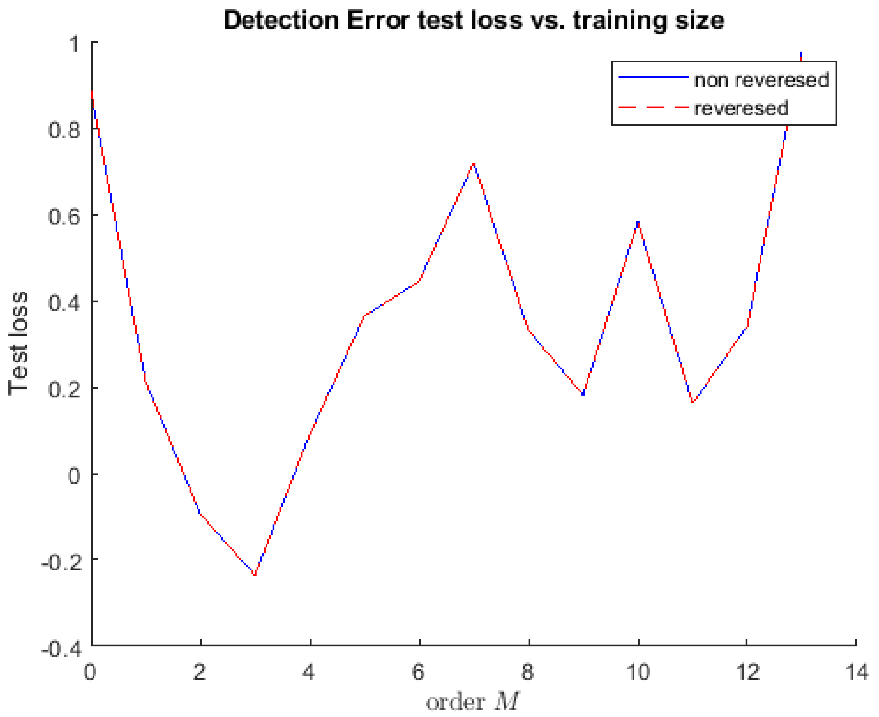
In each specific ensemble element, reversed and nonreversed error detection was compared with the model prediction training size. The order M of each specific ensemble element was denoted by the training size, which represented the spread of information at 70% of the dataset. Meanwhile, values of mean and standard deviation characterized the environment of the specific ensemble element. The test losses indicated the index value of false memories encountered by the population at each iterative training. The nonreversed and reversed curves in Figure 9 show the same acceleration because they occurred at the same time. An object moving with constant acceleration moves with a horizontal line. Zero slope refers to the movement with constant acceleration. The area under the curve shows the change in velocity.

5. Discussion

5.1. Summary of Findings

Computer self-consciousness through RL allows complex ideas that are not possible to render and demonstrate within human conceptions. Understanding the existence of the multiverse is a challenging concept. Establishing theoretical reasoning and experimentation creates the pathway for observing complex phenomena. A representative ensemble can be designed and simulated in several ways. This is because a multiverse is not only limited to a galactic canvas. The planes of space and time can measure instances of the behavior of environments that exist in multiple regions, termed as specific ensemble elements. Each specific ensemble element allows the examination of its policies, agents, controls, critics, observations, rewards, and state spaces. By extracting attributes and categorically exploiting them as parameters for each specific ensemble element, we can observe the range of possibilities for spawning other specific ensemble elements.

The data in this study made use of a binary range, which is the smallest possible range of computational power that can be easily used to design and simulate a functioning representative ensemble. In the multiverse, a very small sample size was chosen for rendition and modeling. Two attributes of each specific ensemble element further narrowed down possible specific ensemble elements that could exist as unique entities. However, a multiverse by no means only has unique entities as described in the design stage. Simulation, however, only deals with unique specific ensemble elements to reduce the complexity of duplicate results affecting the quality.

5.2. Recommendation for Future Work

It was observed that even with only two binary value attributes, the notion of a theoretically possible multiverse consisting of unique specific ensemble elements was computationally demanding. Computing a representative ensemble where multiple copies of each seed’s parameters exist was entirely outside the scope of this research from a computational standpoint. The addition of more parameters with larger intervals (nonbinary) is best suited for computation by supercomputers, which are capable of performing such calculations.

In this study, a lateral scatter-specific ensemble element population was used to populate the representative ensemble. However, it is entirely possible to create a multiverse in several other ways, such as multiple clusters, spirals, sinusoidal, and other shapes on the space plane. Additionally, the behavior on the time plane was modeled cyclically. Other possible ways to model time-based behavior are: particle decay, stochastic probability, and time-based functions. These will allow the measurement of all the other ways a multiverse can exist, thereby increasing the number of possible results. From a human standpoint, such results are impossible to conceive, which is why the results can only be taken advantage of by machines and instruments—in this case, software that can detect health behavior or perceptions and act accordingly.

6. Conclusions

In popular entertainment, the concept of the multiverse has been presented as a possible one. From a computational perspective, simulations can be used to create multiverse scenarios by independently testing the models of each specific ensemble element. Because of the advancements in distributed and parallel computing, the aliasing of the representative ensemble has been greatly improved. Additionally, because of the universe’s mechanism, quantum computers are being developed that can compute the representative ensemble. The goal of this study was to prove the possibility of the multiverse using well-established theories of classical computing. Through parallel computing, each simulated specific ensemble element can independently exist as a parallel reality. However, the engine is not aware that the specific ensemble elements are independent. The complexity of the concept is best conceptualized through computer simulation, and a multiverse can be created theoretically. Representative ensemble causality can be predicted within it, and the Mandela effect can be assumed in this specific ensemble element. To study the behavior of this specific ensemble element, it has to be generated by taking into account the unique specific ensemble elements of a population with two binary attributes. The maximum number of specific ensemble elements that can be generated within the representative ensemble is 182. To minimize the computational effort required to study the specific ensemble elements, the sample count for this study was limited to 606. The parameters used to represent the specific ensemble elements’ attributes were implemented using the $\mu$ and $\sigma$ values. The RL algorithm utilized in the representative ensemble generated different specific ensemble elements. Additionally, a heart attack simulation was performed for each specific ensemble element. The Mandela effect was then tested in each specific ensemble element using the training size of order M. The computers gained a deeper understanding of the specific ensemble element’s parameters, which could represent the possibility of having multiple specific ensemble elements.