Author Contributions
Conceptualization, S.M.A., A.S.H., M.E., I.E., A.M.G. and M.S.; Methodology, S.M.A., A.S.H., M.E., I.E., A.M.G. and M.S.; Formal analysis, S.M.A., A.S.H., M.E., I.E., A.M.G. and M.S.; Writing—original draft, S.M.A., A.S.H., M.E., I.E., A.M.G. and M.S.; Writing—review & editing, S.M.A., A.S.H., M.E., I.E., A.M.G. and M.S. All authors have read and agreed to the published version of the manuscript.
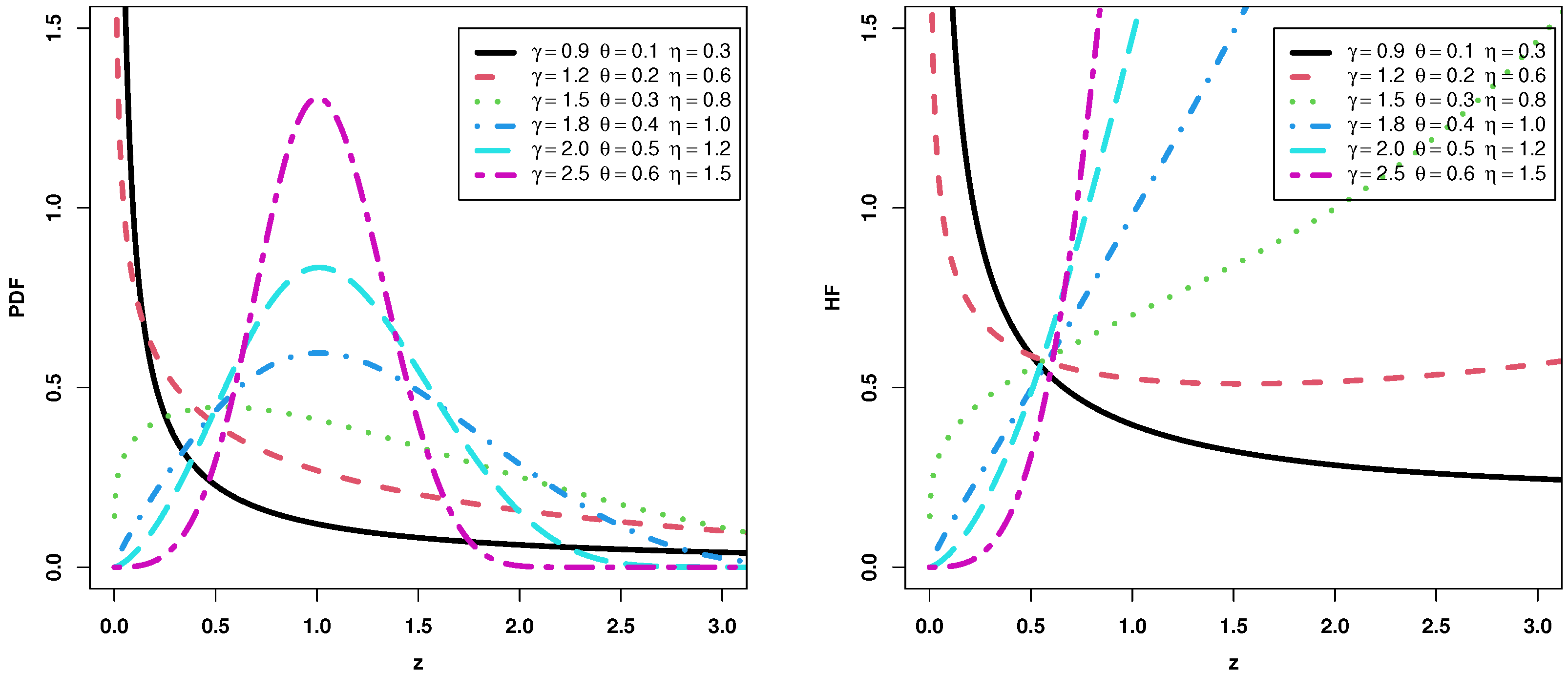
Figure 1.
Plots of the PDF and HF for the HLMKEx model.
Figure 1.
Plots of the PDF and HF for the HLMKEx model.
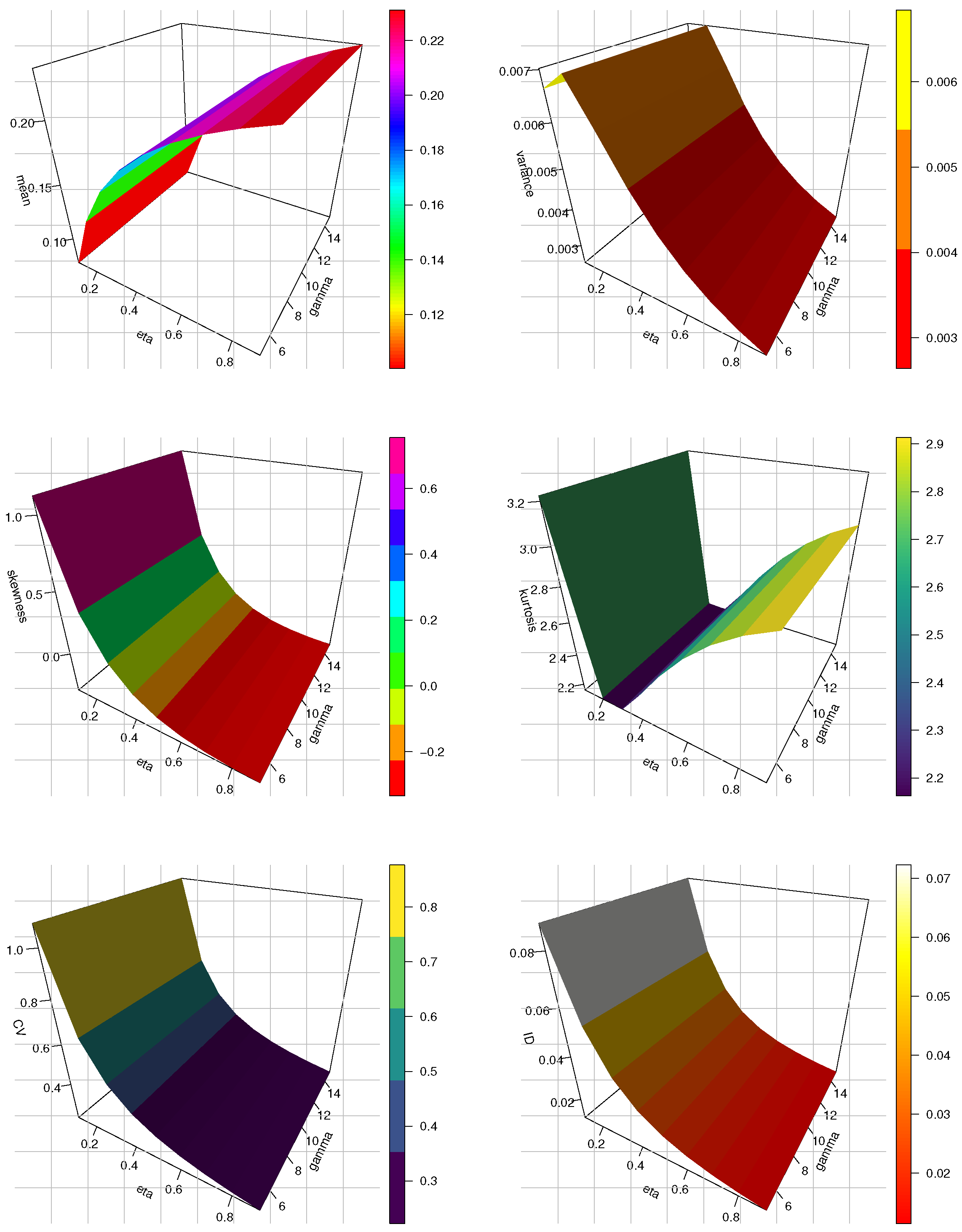
Figure 2.
The 3D plots of mean, variance, SK, KU, CV and ID for the HLMKEx model at .
Figure 2.
The 3D plots of mean, variance, SK, KU, CV and ID for the HLMKEx model at .
Figure 3.
The 3D plots of mean, variance, SK, KU, CV and ID for the HLMKEx model at .
Figure 3.
The 3D plots of mean, variance, SK, KU, CV and ID for the HLMKEx model at .
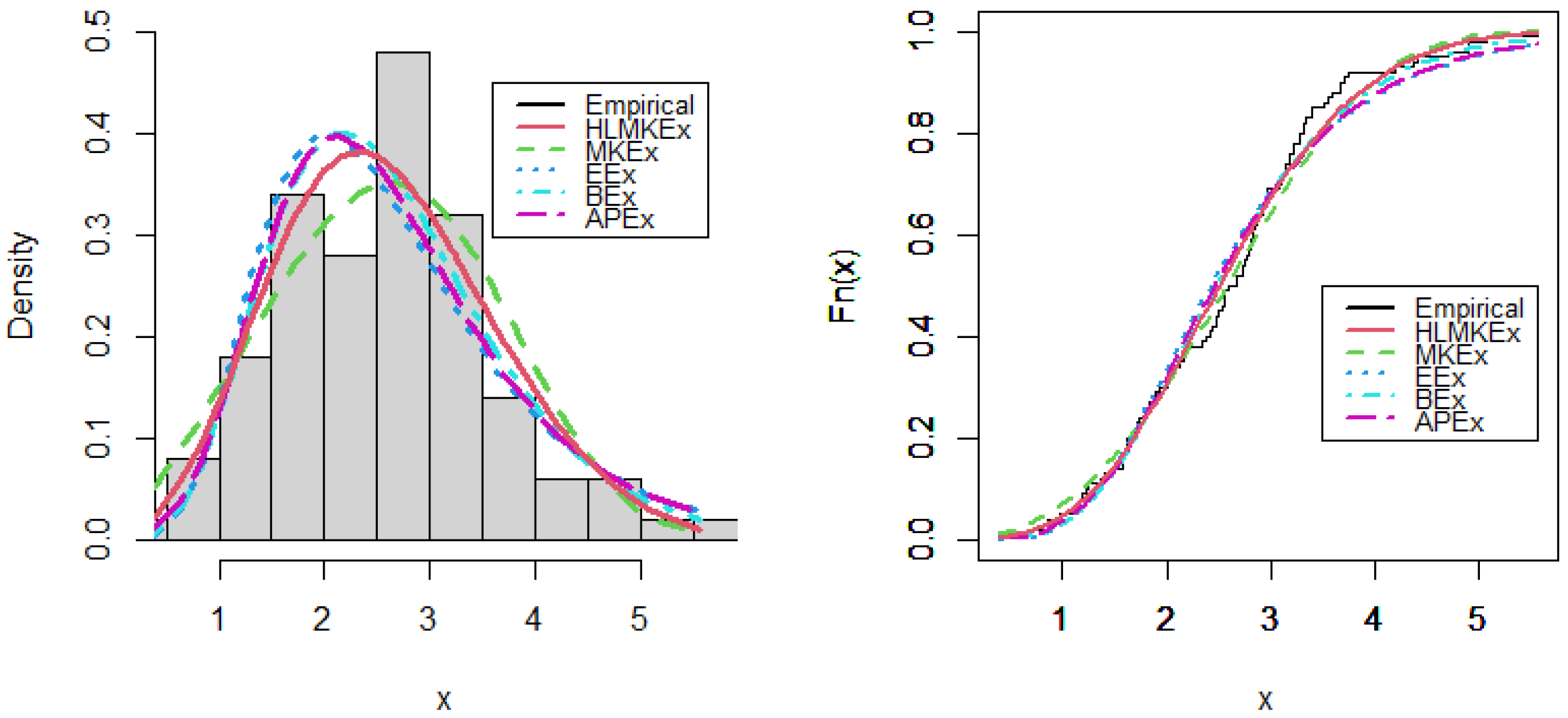
Figure 4.
Estimated PDF and CDF plots of competitive models for breaking stress of carbon fibers data.
Figure 4.
Estimated PDF and CDF plots of competitive models for breaking stress of carbon fibers data.
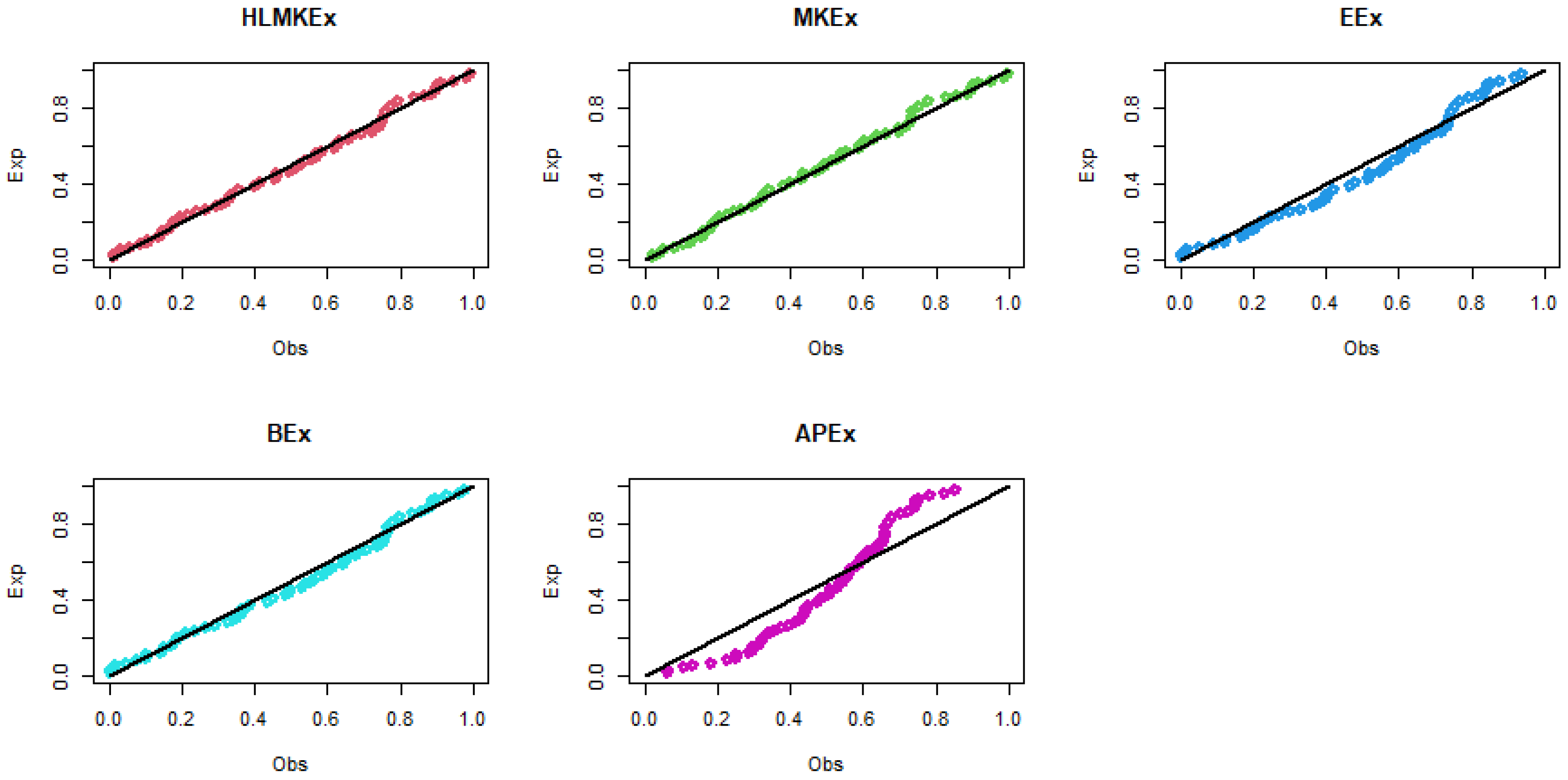
Figure 5.
The P–P plots of the fitted models for breaking stress of carbon fibers data.
Figure 5.
The P–P plots of the fitted models for breaking stress of carbon fibers data.
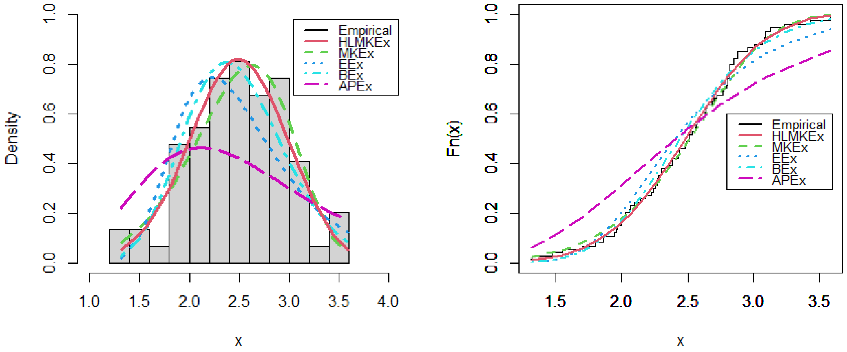
Figure 6.
Estimated PDF and CDF plots of competitive models for gauge lengths data.
Figure 6.
Estimated PDF and CDF plots of competitive models for gauge lengths data.
Figure 7.
The P-P plots of the fitted models for gauge lengths data.
Figure 7.
The P-P plots of the fitted models for gauge lengths data.
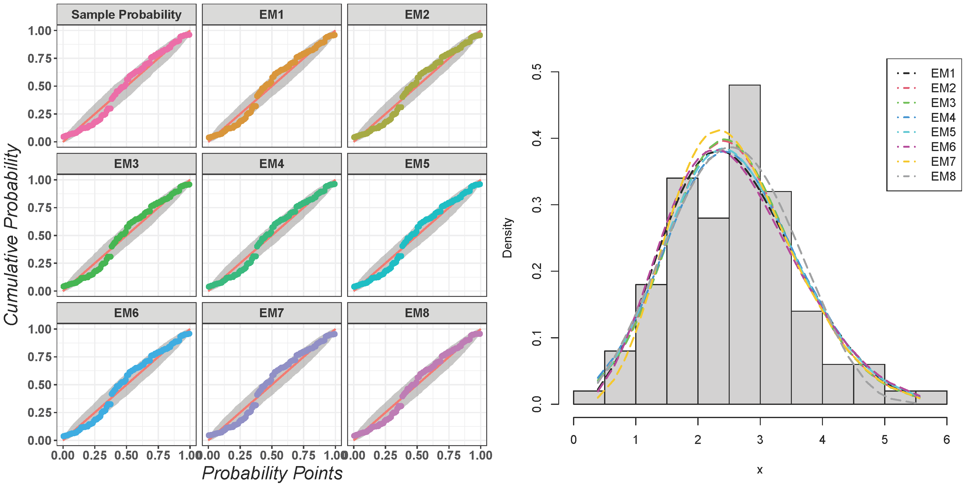
Figure 8.
The P–P plots and the fitted PDFs of the proposed model for the first real data.
Figure 8.
The P–P plots and the fitted PDFs of the proposed model for the first real data.
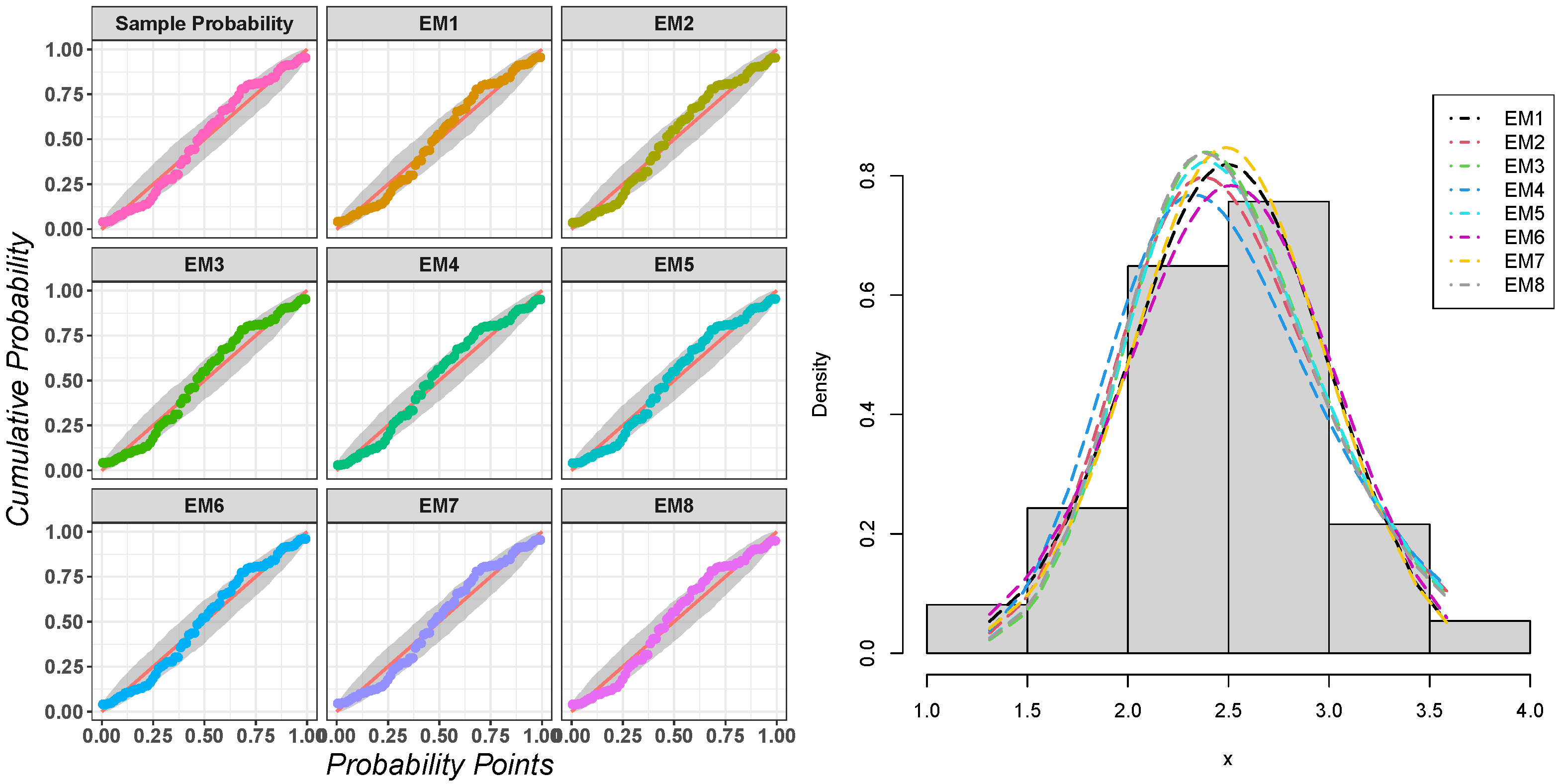
Figure 9.
The P–P plots and the fitted PDFs of the proposed model for the second real data.
Figure 9.
The P–P plots and the fitted PDFs of the proposed model for the second real data.
Table 1.
Results of ,V, CS, CK and CV for the HLMKEx model = 1.2.
Table 1.
Results of ,V, CS, CK and CV for the HLMKEx model = 1.2.
| | | | | | | | | |
|---|
| 0.5 | 0.4 | 0.157 | 0.171 | 0.272 | 0.525 | 0.146 | 3.578 | 17.7 | 2.439 |
| 0.6 | 0.232 | 0.255 | 0.408 | 0.788 | 0.202 | 2.825 | 11.89 | 1.939 |
| 0.8 | 0.303 | 0.339 | 0.543 | 1.05 | 0.247 | 2.371 | 9.054 | 1.64 |
| 1.1 | 0.403 | 0.462 | 0.745 | 1.441 | 0.299 | 1.936 | 6.818 | 1.357 |
| 1.3 | 0.465 | 0.542 | 0.878 | 1.702 | 0.326 | 1.734 | 5.942 | 1.226 |
| 1.7 | 0.579 | 0.699 | 1.142 | 2.219 | 0.363 | 1.444 | 4.871 | 1.041 |
| 1.9 | 0.631 | 0.774 | 1.272 | 2.476 | 0.376 | 1.336 | 4.529 | 0.972 |
| 2.4 | 0.748 | 0.956 | 1.591 | 3.114 | 0.396 | 1.132 | 3.972 | 0.842 |
| 0.8 | 0.4 | 0.163 | 0.11 | 0.108 | 0.129 | 0.084 | 2.608 | 10.56 | 1.773 |
| 0.6 | 0.236 | 0.164 | 0.162 | 0.194 | 0.108 | 2.03 | 7.33 | 1.395 |
| 0.8 | 0.302 | 0.216 | 0.215 | 0.258 | 0.125 | 1.686 | 5.812 | 1.173 |
| 1.1 | 0.388 | 0.291 | 0.294 | 0.353 | 0.14 | 1.364 | 4.669 | 0.966 |
| 1.3 | 0.438 | 0.338 | 0.345 | 0.416 | 0.146 | 1.218 | 4.246 | 0.873 |
| 1.7 | 0.525 | 0.428 | 0.444 | 0.54 | 0.152 | 1.016 | 3.759 | 0.741 |
| 1.9 | 0.563 | 0.47 | 0.492 | 0.601 | 0.152 | 0.943 | 3.616 | 0.693 |
| 2.4 | 0.645 | 0.567 | 0.609 | 0.751 | 0.151 | 0.812 | 3.399 | 0.602 |
| 1 | 0.4 | 0.176 | 0.1 | 0.081 | 0.079 | 0.069 | 2.146 | 7.849 | 1.496 |
| 0.6 | 0.25 | 0.148 | 0.12 | 0.117 | 0.085 | 1.645 | 5.603 | 1.17 |
| 0.8 | 0.314 | 0.193 | 0.159 | 0.156 | 0.095 | 1.351 | 4.585 | 0.981 |
| 1.1 | 0.395 | 0.257 | 0.216 | 0.213 | 0.101 | 1.08 | 3.858 | 0.805 |
| 1.3 | 0.441 | 0.297 | 0.253 | 0.251 | 0.103 | 0.961 | 3.605 | 0.726 |
| 1.7 | 0.518 | 0.37 | 0.323 | 0.324 | 0.102 | 0.8 | 3.337 | 0.617 |
| 1.9 | 0.55 | 0.403 | 0.356 | 0.36 | 0.101 | 0.744 | 3.266 | 0.577 |
| 2.4 | 0.619 | 0.48 | 0.436 | 0.447 | 0.097 | 0.646 | 3.173 | 0.502 |
| 1.3 | 0.4 | 0.197 | 0.097 | 0.065 | 0.051 | 0.058 | 1.645 | 5.487 | 1.217 |
| 0.6 | 0.273 | 0.141 | 0.096 | 0.076 | 0.066 | 1.224 | 4.111 | 0.944 |
| 0.8 | 0.335 | 0.182 | 0.126 | 0.101 | 0.07 | 0.981 | 3.539 | 0.787 |
| 1.1 | 0.41 | 0.238 | 0.169 | 0.137 | 0.07 | 0.765 | 3.181 | 0.643 |
| 1.3 | 0.451 | 0.272 | 0.196 | 0.161 | 0.068 | 0.674 | 3.078 | 0.579 |
| 1.7 | 0.517 | 0.331 | 0.247 | 0.206 | 0.064 | 0.557 | 2.997 | 0.491 |
| 1.9 | 0.544 | 0.358 | 0.271 | 0.227 | 0.062 | 0.519 | 2.986 | 0.459 |
| 2.4 | 0.6 | 0.417 | 0.326 | 0.279 | 0.057 | 0.458 | 2.992 | 0.4 |
| 1.5 | 0.4 | 0.212 | 0.098 | 0.06 | 0.043 | 0.053 | 1.397 | 4.544 | 1.085 |
| 0.6 | 0.288 | 0.142 | 0.089 | 0.065 | 0.058 | 1.012 | 3.53 | 0.837 |
| 0.8 | 0.35 | 0.181 | 0.116 | 0.085 | 0.059 | 0.794 | 3.143 | 0.696 |
| 1.1 | 0.421 | 0.234 | 0.155 | 0.115 | 0.057 | 0.605 | 2.936 | 0.567 |
| 1.3 | 0.459 | 0.265 | 0.178 | 0.134 | 0.055 | 0.528 | 2.893 | 0.51 |
| 1.7 | 0.519 | 0.319 | 0.222 | 0.171 | 0.05 | 0.434 | 2.884 | 0.432 |
| 1.9 | 0.543 | 0.343 | 0.243 | 0.188 | 0.048 | 0.406 | 2.895 | 0.403 |
| 2.4 | 0.593 | 0.395 | 0.289 | 0.229 | 0.043 | 0.363 | 2.934 | 0.351 |
Table 2.
Results of , V, CS, CK and CV for the HLMKEx model = 2.5.
Table 2.
Results of , V, CS, CK and CV for the HLMKEx model = 2.5.
| | | | | | | | | |
|---|
| 0.5 | 0.4 | 0.075 | 0.039 | 0.03 | 0.028 | 0.034 | 3.578 | 17.7 | 2.439 |
| 0.6 | 0.111 | 0.059 | 0.045 | 0.042 | 0.046 | 2.825 | 11.888 | 1.939 |
| 0.8 | 0.145 | 0.078 | 0.06 | 0.056 | 0.057 | 2.371 | 9.054 | 1.64 |
| 1.1 | 0.194 | 0.106 | 0.082 | 0.077 | 0.069 | 1.936 | 6.818 | 1.357 |
| 1.3 | 0.223 | 0.125 | 0.097 | 0.09 | 0.075 | 1.734 | 5.942 | 1.226 |
| 1.7 | 0.278 | 0.161 | 0.126 | 0.118 | 0.084 | 1.444 | 4.871 | 1.041 |
| 1.9 | 0.303 | 0.178 | 0.141 | 0.131 | 0.087 | 1.336 | 4.529 | 0.972 |
| 2.4 | 0.359 | 0.22 | 0.176 | 0.165 | 0.091 | 1.132 | 3.972 | 0.842 |
| 0.8 | 0.4 | 0.078 | 0.025 | 0.012 | 0.0069 | 0.019 | 2.608 | 10.555 | 1.773 |
| 0.6 | 0.113 | 0.038 | 0.018 | 0.01 | 0.025 | 2.03 | 7.33 | 1.395 |
| 0.8 | 0.145 | 0.05 | 0.024 | 0.014 | 0.029 | 1.686 | 5.811 | 1.173 |
| 1.1 | 0.186 | 0.067 | 0.032 | 0.019 | 0.032 | 1.364 | 4.669 | 0.966 |
| 1.3 | 0.21 | 0.078 | 0.038 | 0.022 | 0.034 | 1.218 | 4.246 | 0.873 |
| 1.7 | 0.252 | 0.099 | 0.049 | 0.029 | 0.035 | 1.016 | 3.759 | 0.741 |
| 1.9 | 0.27 | 0.108 | 0.054 | 0.032 | 0.035 | 0.943 | 3.616 | 0.693 |
| 2.4 | 0.31 | 0.131 | 0.067 | 0.04 | 0.035 | 0.812 | 3.399 | 0.602 |
| 1 | 0.4 | 0.084 | 0.023 | 0.0089 | 0.0042 | 0.016 | 2.146 | 7.856 | 1.496 |
| 0.6 | 0.12 | 0.034 | 0.013 | 0.0062 | 0.02 | 1.645 | 5.603 | 1.17 |
| 0.8 | 0.151 | 0.044 | 0.018 | 0.0083 | 0.022 | 1.351 | 4.585 | 0.981 |
| 1.1 | 0.19 | 0.059 | 0.024 | 0.011 | 0.023 | 1.08 | 3.858 | 0.805 |
| 1.3 | 0.212 | 0.068 | 0.028 | 0.013 | 0.024 | 0.961 | 3.605 | 0.727 |
| 1.7 | 0.248 | 0.085 | 0.036 | 0.017 | 0.023 | 0.8 | 3.337 | 0.617 |
| 1.9 | 0.264 | 0.093 | 0.039 | 0.019 | 0.023 | 0.744 | 3.266 | 0.577 |
| 2.4 | 0.297 | 0.111 | 0.048 | 0.024 | 0.022 | 0.646 | 3.173 | 0.502 |
| 1.3 | 0.4 | 0.095 | 0.022 | 0.0071 | 0.0027 | 0.013 | 1.645 | 5.487 | 1.217 |
| 0.6 | 0.131 | 0.032 | 0.011 | 0.004 | 0.015 | 1.224 | 4.111 | 0.944 |
| 0.8 | 0.161 | 0.042 | 0.014 | 0.0054 | 0.016 | 0.981 | 3.539 | 0.787 |
| 1.1 | 0.197 | 0.055 | 0.019 | 0.0073 | 0.016 | 0.765 | 3.181 | 0.643 |
| 1.3 | 0.216 | 0.063 | 0.022 | 0.0085 | 0.016 | 0.674 | 3.078 | 0.579 |
| 1.7 | 0.248 | 0.076 | 0.027 | 0.011 | 0.015 | 0.557 | 2.997 | 0.491 |
| 1.9 | 0.261 | 0.083 | 0.03 | 0.012 | 0.014 | 0.519 | 2.986 | 0.459 |
| 2.4 | 0.288 | 0.096 | 0.036 | 0.015 | 0.013 | 0.458 | 2.992 | 0.4 |
| 1.5 | 0.4 | 0.102 | 0.023 | 0.00665 | 0.00038 | 0.012 | 1.397 | 4.559 | 1.085 |
| 0.6 | 0.138 | 0.033 | 0.0098 | 0.0034 | 0.013 | 1.012 | 3.53 | 0.837 |
| 0.8 | 0.168 | 0.042 | 0.013 | 0.0045 | 0.014 | 0.794 | 3.143 | 0.696 |
| 1.1 | 0.202 | 0.054 | 0.017 | 0.0061 | 0.013 | 0.605 | 2.936 | 0.567 |
| 1.3 | 0.22 | 0.061 | 0.02 | 0.0071 | 0.013 | 0.528 | 2.893 | 0.51 |
| 1.7 | 0.249 | 0.074 | 0.025 | 0.0091 | 0.012 | 0.434 | 2.884 | 0.432 |
| 1.9 | 0.261 | 0.079 | 0.027 | 0.00997 | 0.011 | 0.406 | 2.895 | 0.403 |
| 2.4 | 0.285 | 0.091 | 0.032 | 0.012 | 0.01 | 0.363 | 2.934 | 0.351 |
Table 3.
Simulation values of BIAS, MSE and MRE for .
Table 3.
Simulation values of BIAS, MSE and MRE for .
| n | Measures | | | | | | | | | |
|---|
| 75 | BIAS | | | | | | | | | |
| | | | | | | | |
| | | | | | | | |
| MSE | | | | | | | | | |
| | | | | | | | |
| | | | | | | | |
| MRE | | | | | | | | | |
| | | | | | | | |
| | | | | | | | |
| | | | | | | | | |
| 120 | BIAS | | | | | | | | | |
| | | | | | | | |
| | | | | | | | |
| MSE | | | | | | | | | |
| | | | | | | | |
| | | | | | | | |
| MRE | | | | | | | | | |
| | | | | | | | |
| | | | | | | | |
| | | | | | | | | |
| 150 | BIAS | | | | | | | | | |
| | | | | | | | |
| | | | | | | | |
| MSE | | | | | | | | | |
| | | | | | | | |
| | | | | | | | |
| MRE | | | | | | | | | |
| | | | | | | | |
| | | | | | | | |
| | | | | | | | | |
| 200 | BIAS | | | | | | | | | |
| | | | | | | | |
| | | | | | | | |
| MSE | | | | | | | | | |
| | | | | | | | |
| | | | | | | | |
| MRE | | | | | | | | | |
| | | | | | | | |
| | | | | | | | |
| | | | | | | | | |
| 300 | BIAS | | | | | | | | | |
| | | | | | | | |
| | | | | | | | |
| MSE | | | | | | | | | |
| | | | | | | | |
| | | | | | | | |
| MRE | | | | | | | | | |
| | | | | | | | |
| | | | | | | | |
| | | | | | | | | |
Table 4.
Simulation values of BIAS, MSE and MRE for .
Table 4.
Simulation values of BIAS, MSE and MRE for .
| n | Measures | | | | | | | | | |
|---|
| 75 | BIAS | | | | | | | | | |
| | | | | | | | |
| | | | | | | | |
| MSE | | | | | | | | | |
| | | | | | | | |
| | | | | | | | |
| MRE | | | | | | | | | |
| | | | | | | | |
| | | | | | | | |
| | | | | | | | | |
| 120 | BIAS | | | | | | | | | |
| | | | | | | | |
| | | | | | | | |
| MSE | | | | | | | | | |
| | | | | | | | |
| | | | | | | | |
| MRE | | | | | | | | | |
| | | | | | | | |
| | | | | | | | |
| | | | | | | | | |
| 150 | BIAS | | | | | | | | | |
| | | | | | | | |
| | | | | | | | |
| MSE | | | | | | | | | |
| | | | | | | | |
| | | | | | | | |
| MRE | | | | | | | | | |
| | | | | | | | |
| | | | | | | | |
| | | | | | | | | |
| 200 | BIAS | | | | | | | | | |
| | | | | | | | |
| | | | | | | | |
| MSE | | | | | | | | | |
| | | | | | | | |
| | | | | | | | |
| MRE | | | | | | | | | |
| | | | | | | | |
| | | | | | | | |
| | | | | | | | | |
| 300 | BIAS | | | | | | | | | |
| | | | | | | | |
| | | | | | | | |
| MSE | | | | | | | | | |
| | | | | | | | |
| | | | | | | | |
| MRE | | | | | | | | | |
| | | | | | | | |
| | | | | | | | |
| | | | | | | | | |
Table 5.
Simulation values of BIAS, MSE and MRE for .
Table 5.
Simulation values of BIAS, MSE and MRE for .
| n | Measures | | | | | | | | | |
|---|
| 75 | BIAS | | | | | | | | | |
| | | | | | | | |
| | | | | | | | |
| MSE | | | | | | | | | |
| | | | | | | | |
| | | | | | | | |
| MRE | | | | | | | | | |
| | | | | | | | |
| | | | | | | | |
| | | | | | | | | |
| 120 | BIAS | | | | | | | | | |
| | | | | | | | |
| | | | | | | | |
| MSE | | | | | | | | | |
| | | | | | | | |
| | | | | | | | |
| MRE | | | | | | | | | |
| | | | | | | | |
| | | | | | | | |
| | | | | | | | | |
| 150 | BIAS | | | | | | | | | |
| | | | | | | | |
| | | | | | | | |
| MSE | | | | | | | | | |
| | | | | | | | |
| | | | | | | | |
| MRE | | | | | | | | | |
| | | | | | | | |
| | | | | | | | |
| | | | | | | | | |
| 200 | BIAS | | | | | | | | | |
| | | | | | | | |
| | | | | | | | |
| MSE | | | | | | | | | |
| | | | | | | | |
| | | | | | | | |
| MRE | | | | | | | | | |
| | | | | | | | |
| | | | | | | | |
| | | | | | | | | |
| 300 | BIAS | | | | | | | | | |
| | | | | | | | |
| | | | | | | | |
| MSE | | | | | | | | | |
| | | | | | | | |
| | | | | | | | |
| MRE | | | | | | | | | |
| | | | | | | | |
| | | | | | | | |
| | | | | | | | | |
Table 6.
Simulation values of BIAS, MSE and MRE for .
Table 6.
Simulation values of BIAS, MSE and MRE for .
| n | Measures | | | | | | | | | |
|---|
| 75 | BIAS | | | | | | | | | |
| | | | | | | | |
| | | | | | | | |
| MSE | | | | | | | | | |
| | | | | | | | |
| | | | | | | | |
| MRE | | | | | | | | | |
| | | | | | | | |
| | | | | | | | |
| | | | | | | | | |
| 120 | BIAS | | | | | | | | | |
| | | | | | | | |
| | | | | | | | |
| MSE | | | | | | | | | |
| | | | | | | | |
| | | | | | | | |
| MRE | | | | | | | | | |
| | | | | | | | |
| | | | | | | | |
| | | | | | | | | |
| 150 | BIAS | | | | | | | | | |
| | | | | | | | |
| | | | | | | | |
| MSE | | | | | | | | | |
| | | | | | | | |
| | | | | | | | |
| MRE | | | | | | | | | |
| | | | | | | | |
| | | | | | | | |
| | | | | | | | | |
| 200 | BIAS | | | | | | | | | |
| | | | | | | | |
| | | | | | | | |
| MSE | | | | | | | | | |
| | | | | | | | |
| | | | | | | | |
| MRE | | | | | | | | | |
| | | | | | | | |
| | | | | | | | |
| | | | | | | | | |
| 300 | BIAS | | | | | | | | | |
| | | | | | | | |
| | | | | | | | |
| MSE | | | | | | | | | |
| | | | | | | | |
| | | | | | | | |
| MRE | | | | | | | | | |
| | | | | | | | |
| | | | | | | | |
| | | | | | | | | |
Table 7.
Simulation values of BIAS, MSE and MRE for .
Table 7.
Simulation values of BIAS, MSE and MRE for .
| n | Measures | | | | | | | | | |
|---|
| 75 | BIAS | | | | | | | | | |
| | | | | | | | |
| | | | | | | | |
| MSE | | | | | | | | | |
| | | | | | | | |
| | | | | | | | |
| MRE | | | | | | | | | |
| | | | | | | | |
| | | | | | | | |
| | | | | | | | | |
| 120 | BIAS | | | | | | | | | |
| | | | | | | | |
| | | | | | | | |
| MSE | | | | | | | | | |
| | | | | | | | |
| | | | | | | | |
| MRE | | | | | | | | | |
| | | | | | | | |
| | | | | | | | |
| | | | | | | | | |
| 150 | BIAS | | | | | | | | | |
| | | | | | | | |
| | | | | | | | |
| MSE | | | | | | | | | |
| | | | | | | | |
| | | | | | | | |
| MRE | | | | | | | | | |
| | | | | | | | |
| | | | | | | | |
| | | | | | | | | |
| 200 | BIAS | | | | | | | | | |
| | | | | | | | |
| | | | | | | | |
| MSE | | | | | | | | | |
| | | | | | | | |
| | | | | | | | |
| MRE | | | | | | | | | |
| | | | | | | | |
| | | | | | | | |
| | | | | | | | | |
| 300 | BIAS | | | | | | | | | |
| | | | | | | | |
| | | | | | | | |
| MSE | | | | | | | | | |
| | | | | | | | |
| | | | | | | | |
| MRE | | | | | | | | | |
| | | | | | | | |
| | | | | | | | |
| | | | | | | | | |
Table 8.
Simulation values of BIAS, MSE and MRE for .
Table 8.
Simulation values of BIAS, MSE and MRE for .
| n | Measures | | | | | | | | | |
|---|
| 75 | BIAS | | | | | | | | | |
| | | | | | | | |
| | | | | | | | |
| MSE | | | | | | | | | |
| | | | | | | | |
| | | | | | | | |
| MRE | | | | | | | | | |
| | | | | | | | |
| | | | | | | | |
| | | | | | | | | |
| 120 | BIAS | | | | | | | | | |
| | | | | | | | |
| | | | | | | | |
| MSE | | | | | | | | | |
| | | | | | | | |
| | | | | | | | |
| MRE | | | | | | | | | |
| | | | | | | | |
| | | | | | | | |
| | | | | | | | | |
| 150 | BIAS | | | | | | | | | |
| | | | | | | | |
| | | | | | | | |
| MSE | | | | | | | | | |
| | | | | | | | |
| | | | | | | | |
| MRE | | | | | | | | | |
| | | | | | | | |
| | | | | | | | |
| | | | | | | | | |
| 200 | BIAS | | | | | | | | | |
| | | | | | | | |
| | | | | | | | |
| MSE | | | | | | | | | |
| | | | | | | | |
| | | | | | | | |
| MRE | | | | | | | | | |
| | | | | | | | |
| | | | | | | | |
| | | | | | | | | |
| 300 | BIAS | | | | | | | | | |
| | | | | | | | |
| | | | | | | | |
| MSE | | | | | | | | | |
| | | | | | | | |
| | | | | | | | |
| MRE | | | | | | | | | |
| | | | | | | | |
| | | | | | | | |
| | | | | | | | | |
Table 9.
Partial and overall ranks of all the methods of estimation of proposed distribution by various values of model parameters.
Table 9.
Partial and overall ranks of all the methods of estimation of proposed distribution by various values of model parameters.
| Parameter | n | | | | | | | | |
|---|
| 75 | 4.0 | 3.0 | 8.0 | 1.0 | 7.0 | 6.0 | 2.0 | 5.0 |
| 120 | 5.0 | 3.0 | 8.0 | 1.0 | 7.0 | 4.0 | 2.0 | 6.0 |
| 150 | 4.5 | 3.0 | 8.0 | 1.0 | 7.0 | 4.5 | 2.0 | 6.0 |
| 200 | 4.5 | 3.0 | 8.0 | 1.0 | 7.0 | 4.5 | 2.0 | 6.0 |
| 300 | 3.0 | 5.0 | 7.0 | 1.0 | 8.0 | 4.0 | 2.0 | 6.0 |
| 75 | 1.0 | 2.0 | 6.5 | 5.0 | 6.5 | 8.0 | 3.0 | 4.0 |
| 120 | 1.0 | 2.0 | 5.5 | 5.5 | 7.0 | 8.0 | 3.5 | 3.5 |
| 150 | 1.0 | 4.0 | 7.0 | 5.0 | 6.0 | 8.0 | 2.0 | 3.0 |
| 200 | 1.0 | 3.0 | 6.0 | 5.0 | 7.0 | 8.0 | 2.0 | 4.0 |
| 300 | 1.0 | 2.0 | 7.0 | 5.0 | 6.0 | 8.0 | 4.0 | 3.0 |
| 75 | 2.0 | 3.0 | 7.0 | 1.0 | 5.0 | 8.0 | 6.0 | 4.0 |
| 120 | 2.0 | 3.0 | 7.0 | 1.0 | 6.0 | 8.0 | 5.0 | 4.0 |
| 150 | 1.0 | 3.0 | 7.0 | 2.0 | 6.0 | 8.0 | 5.0 | 4.0 |
| 200 | 1.5 | 3.0 | 6.0 | 1.5 | 7.0 | 8.0 | 5.0 | 4.0 |
| 300 | 5.0 | 1.5 | 6.0 | 3.0 | 7.0 | 8.0 | 4.0 | 1.5 |
| 75 | 5.0 | 2.0 | 8.0 | 1.0 | 7.0 | 3.0 | 6.0 | 4.0 |
| 120 | 6.0 | 2.0 | 8.0 | 1.0 | 7.0 | 4.0 | 3.0 | 5.0 |
| 150 | 3.0 | 2.0 | 8.0 | 1.0 | 7.0 | 5.0 | 4.0 | 6.0 |
| 200 | 2.0 | 3.0 | 8.0 | 1.0 | 7.0 | 5.0 | 6.0 | 4.0 |
| 300 | 2.0 | 4.0 | 7.0 | 1.0 | 8.0 | 6.0 | 5.0 | 3.0 |
| 75 | 5.0 | 3.0 | 8.0 | 1.0 | 6.0 | 2.0 | 7.0 | 4.0 |
| 120 | 2.0 | 3.0 | 8.0 | 1.0 | 7.0 | 4.0 | 6.0 | 5.0 |
| 150 | 2.0 | 3.0 | 8.0 | 1.0 | 7.0 | 4.0 | 6.0 | 5.0 |
| 200 | 2.0 | 3.0 | 7.5 | 1.0 | 6.0 | 4.0 | 7.5 | 5.0 |
| 300 | 2.0 | 3.0 | 8.0 | 1.0 | 6.0 | 4.0 | 7.0 | 5.0 |
| 75 | 7.0 | 4.0 | 8.0 | 1.0 | 6.0 | 2.0 | 3.0 | 5.0 |
| 120 | 8.0 | 3.0 | 6.5 | 1.0 | 6.5 | 2.0 | 4.0 | 5.0 |
| 150 | 6.0 | 3.0 | 7.5 | 1.0 | 7.5 | 2.0 | 5.0 | 4.0 |
| 200 | 7.0 | 4.0 | 8.0 | 1.0 | 6.0 | 2.0 | 3.0 | 5.0 |
| 300 | 7.0 | 3.0 | 8.0 | 1.0 | 6.0 | 2.0 | 4.0 | 5.0 |
| ∑ Ranks | | 103.5 | 88.5 | 220.5 | 54.0 | 199.5 | 154.0 | 126.0 | 134.0 |
| Overall Rank | | 3 | 2 | 8 | 1 | 7 | 6 | 4 | 5 |
Table 10.
Some descriptive analyses of all data sets.
Table 10.
Some descriptive analyses of all data sets.
| | n | Mean | Median | Skewness | Kurtosis | Range | Minimum | Maximum | Sum |
|---|
| data1 | 100 | 2.5814 | 2.63 | 0.3893 | 0.25467 | 5.17 | 0.39 | 5.56 | 258.14 |
| data2 | 74 | 2.4773 | 2.5125 | −0.1574 | 0.03345 | 2.273 | 1.312 | 3.585 | 183.318 |
Table 11.
The WST, AST, KOS, KOSP, MLEs, and SEs for breaking stress of carbon fibers data.
Table 11.
The WST, AST, KOS, KOSP, MLEs, and SEs for breaking stress of carbon fibers data.
| Distribution | WST | AST | KOS | KOSP | | Estimates (SEs) |
|---|
| HLMKEx | 0.09202 | 0.51764 | 0.0673 | 0.7552 | | 1.637 (0.652) |
| 1.718 (1.0059) |
| 0.2423 (0.0542) |
| MKEx | 0.17398 | 0.61251 | 0.08574 | 0.4542 | | 1.966 (0.1548) |
| 0.2334 (0.00887) |
| EEx | 0.226 | 0.585 | 0.1077 | 0.1962 | | 7.7882 (1.496) |
| 1.0132 (0.087) |
| BEx | 0.148 | 0.758 | 0.0935 | 0.3461 | a | 5.9605 (0.821) |
| b | 34.5462 (61.141) |
| 0.0615 (0.102) |
| APEx | 0.184 | 0.939 | 0.0954 | 0.3228 | | 19,134.8 (8983) |
| 1.0777 (0.0509) |
Table 12.
The WST, AST, KOS, KOSP, MLEs, and SEs for gauge lengths data.
Table 12.
The WST, AST, KOS, KOSP, MLEs, and SEs for gauge lengths data.
| Distribution | WST | AST | KOS | KOSP | | Estimates (SEs) |
|---|
| HLMKEx | 0.03002 | 0.22883 | 0.0602 | 0.9512 | | 3.652 (1.343) |
| 1.577 (0.908) |
| 0.259 (0.0261) |
| MKEx | 0.03215 | 0.30334 | 0.0753 | 0.7954 | | 4.152 (0.371) |
| 0.258 (0.0055) |
| EEx | 0.2172 | 1.4053 | 0.0953 | 0.5121 | | 89.435 (32.476) |
| 2.0192 (0.1716) |
| BEx | 0.0874 | 0.5738 | 0.0682 | 0.8809 | a | 24.317 (3.9884) |
| b | 92.491 (154.90) |
| 0.0947 (0.1426) |
| APEx | 0.1153 | 0.7486 | 0.1924 | 0.0083 | | 1,592,046 (16777) |
| 1.2536 (0.0549) |
Table 13.
Estimated parameters with goodness-of-fit measures by different estimation methods for the breaking stress of carbon fibers data set.
Table 13.
Estimated parameters with goodness-of-fit measures by different estimation methods for the breaking stress of carbon fibers data set.
| Method | | | | AST | WST | KOS | KOSP |
|---|
| 0.2423 | 1.718 | 1.637 | 0.51764 | 0.09202 | 0.0673 | 0.7552 |
| 1.99373 | 12.8273 | 0.182177 | 0.4415 | 0.0749703 | 0.0618446 | 0.838957 |
| 2.39286 | 13.0523 | 0.152564 | 0.439598 | 0.0731711 | 0.0604884 | 0.857751 |
| 1.93992 | 12.2451 | 0.182529 | 0.491826 | 0.0815856 | 0.0715943 | 0.684557 |
| 1.56649 | 12.0819 | 0.226449 | 0.470536 | 0.080918 | 0.0678114 | 0.747293 |
| 0.267448 | 2.1967 | 1.37191 | 0.541278 | 0.0993827 | 0.0733148 | 0.655578 |
| 0.28814 | 2.67928 | 1.30599 | 0.64157 | 0.094863 | 0.0632017 | 0.81927 |
| 0.199022 | 0.780023 | 3.04153 | 0.668256 | 0.0599927 | 0.0562461 | 0.909759 |
Table 14.
Estimated parameters with goodness-of-fit measures by different estimation methods for the gauge lengths real data set.
Table 14.
Estimated parameters with goodness-of-fit measures by different estimation methods for the gauge lengths real data set.
| Method | | | | AST | WST | KOS | KOSP |
|---|
| 0.259 | 1.577 | 3.652 | 0.22883 | 0.03002 | 0.0602 | 0.9512 |
| 2.57578 | 39.7856 | 0.20216 | 0.527451 | 0.067717 | 0.0743585 | 0.807842 |
| 26.1644 | 45.1059 | 0.0203112 | 0.536762 | 0.0566676 | 0.0709002 | 0.8509 |
| 0.688956 | 19.3123 | 0.721908 | 0.772891 | 0.117443 | 0.0740044 | 0.812428 |
| 25.6194 | 43.215 | 0.0205635 | 0.524675 | 0.0575394 | 0.0748339 | 0.801631 |
| 0.251169 | 1.33358 | 3.92256 | 0.258384 | 0.0337077 | 0.0694041 | 0.868182 |
| 0.266217 | 1.87355 | 3.38647 | 0.249827 | 0.0303681 | 0.0555073 | 0.97655 |
| 21.2889 | 44.3588 | 0.0250144 | 0.506376 | 0.0618432 | 0.0643198 | 0.919464 |


 ,
, 


