Coherent Plasma in a Lattice

Abstract

We present a fully second-quantized calculation showing the emergence of spontaneous coherent configurations of the electromagnetic field interacting with charged bosons in a regular lattice. The bosons tend to oscillate at their plasma frequency, and in addition are subjected to electrostatic forces which keep them confined close to the lattice sites while causing a frequency shift in the oscillation. Under certain conditions upon these frequencies, we find that a suitably defined set of coherent states (coherent both in the field and matter degrees of freedom) exhibit a negative energy gap with respect to the perturbative ground state. This is true in the RWA approximation and for position-independent fields to both the first and second order in the interaction Hamiltonian. We compare this result with other recent findings from cavity QED, and note that (1) consideration of full 3D wavefunctions and a careful definition of the coherent states are essential for obtaining the energy gap, and (2) although our calculation is made in reference to bosons, it may apply to protons bound in a crystal matrix as well if their density is very low compared to the density of available states.

1. Introduction

The stability of the perturbative ground state in single-mode cavity QED has been intensively studied under broad conditions for quantum gases and electron systems [1,2,3,4,5,6,7,8,9], when the diamagnetic term proportional to ${\mathbf{A}}^2$ is taken into account or not (the so-called “no-go theorem” for the superradiant transition in its various versions; see [2,10]). The control, at a microscopic level, of coherent interactions between light and matter is one of the main focus points of quantum technologies. In this context, methods for increasing the light—matter coupling strength acquire special importance. As long as the coupling strength remains much smaller than the frequency of the cavity mode, only the resonant terms in the interaction Hamiltonian play a significant role. The remaining counter-rotating terms couple states with contributions that can be neglected. The so-called rotating-wave approximation (RWA) provides an accurate picture of atom–photon interaction processes in this regime [11,12,13].

There are other important cases in quantum field theory in which the perturbative ground state is unstable, e.g., in QCD [14,15,16] and quantum gravity [17,18,19,20,21]. Such instabilities are usually related to complex dynamical behavior not reducible to single-particle excitations. This can lead to the formation of so-called “kinetic condensates”, differing from the more common translationally invariant potential condensates related to the conventional Higgs mechanism.

In this work, we consider an idealized physical system of localized oscillating charges coupled to a multi-mode monochromatic electromagnetic field in which a finite energy gap develops at zero temperature; we compute it rigorously using a set of trial states which are coherent in both the matter and field sectors. In this calculation, the ${\mathbf{A}}^2$ term is included and no-go theorems are avoided, as we consider electromagnetic modes with their momenta quantized in all possible directions. These modes are confined in the material due to a dispersion relation $k\left(\omega \right)$ that prevents them from escaping even in the absence of an external cavity.

Of course, there are conditions that need to be satisfied for a negative gap, especially concerning the relation between the plasma frequency ${\omega }_p$ and another characteristic frequency $\omega$ that defines the strength of the electrostatic potential binding the charges to the lattice sites.

In Section 2, we introduce the Hamiltonian of the system, which contains the kinetic term of the bosons in the presence of a vector potential, plus the Hamiltonian of free cavity photons of momentum $\overrightarrow{k}$ (with $|\overrightarrow{k}|=\omega$) and a harmonic potential due to the combined effect of plasma oscillations and of local electrostatic “cages” near each lattice site. In real systems, these cages typically correspond to tetrahedral or octahedral holes [22]. In agreement with standard approaches for handling the diamagnetic term [9,23], we define new photon operators with the same momentum $\overrightarrow{k}$ and a shifted or “dressed” frequency ${\omega }^{\prime }=\sqrt{{\omega }^2+{\omega }_p^2}$ equal to the oscillation frequency of the matter field (see Appendix B). The interaction term is written employing the dipole approximation, i.e., with the vector potential constant in space.

In Section 3, we define photon operators which project along the three space directions via a canonical transformation in preparation for the introduction of trial coherent states $|\mathrm{\Omega }\rangle$ in which matter oscillations occur in one specific direction (Section 4). The full Hamiltonian, when evaluated on these trial states in the rotating wave approximation (RWA), reduces to an effective Hamiltonian with a minimum that exhibits an energy gap per particle of the form $\delta E_{\mathrm{\Omega }}^{\left(1\right)}={\omega }^{\prime }{\left|\alpha \right|}^2\left(1-\frac{2\pi }{3}{\epsilon }^2\right)$, where $\epsilon ={\omega }_p/{\omega }^{\prime }$, meaning that the perturbative vacuum becomes unstable at the first order when $\epsilon >{\epsilon }_{\mathrm{crit}}\simeq 0.69$.

The factor $\left|\alpha \right|$ in the gap formula controls the oscillation amplitude in the trial coherent state, which is physically limited by the lattice spacing (Section 5). In Section 6 and Section 7, we compute the contribution to the energy gap provided by the second perturbative order in the interaction Hamiltonian describing processes in which photons are emitted and re-absorbed at different lattice sites. The resulting expression for the gap up to second order is very similar, namely, $\delta E_{\mathrm{\Omega }}^{\left(2\right)}={\omega }^{\prime }{\left|\alpha \right|}^2\left(1-\frac{8\pi }{3}{\epsilon }^2\right)$, implying condensation for even lower values of the coupling constant $\epsilon >{\epsilon }_{\mathrm{crit}}\simeq 0.35$.

In Appendix D, we provide a numerical estimate of the condensation threshold and of the energy gap for a realistic case, namely, for protons absorbed into an FCC metallic matrix, when their density is so low that they can be described by a bosonic wavefunction. Supposing one proton per lattice site and a lattice spacing $d=2.5\mathrm{\AA }$, we obtain a coupling constant $\epsilon =0.56>{\epsilon }_{\mathrm{crit}}\simeq 0.35$. Thus, the system is over threshold and condensation occurs under robust conditions. Assuming that the amplitude of the oscillation is fixed by the size of the octahedral sites of the crystal, the average energy gap per particle is $\delta E_{\mathrm{\Omega }}^{\left(2\right)}\simeq -1$ eV and the frequencies $\omega$ and ${\omega }_p$ are in the THz range, which is in good agreement with the values of the largest phonon frequencies adapted to the proton mass [24].

In Section 8, we estimate the spatial dependence of the field and argue that coherence domains form, at the boundary of which the field decreases in keeping with the spherical Bessel function $j_0\left(r\right)$.

Section 9 contains a final discussion and outlook on future work. From the historical point of view, we point out that extensive pioneering work on e.m. coherence in condensed matter was carried out in the 1990s by G. Preparata [25], who introduced the concept of coherence domains. Our present approach was inspired by Preparata’s work; however, it is independent from it and completely self-consistent.

The main results of this paper are summarized in Section 10.

In addition to the mentioned Appendix B and Appendix D, Appendix C and Appendix E contain technical details of the calculation. In Appendix A, a static charge distribution is defined which reproduces the almost-harmonic potential used in the Hamiltonian.

2. Hamiltonian

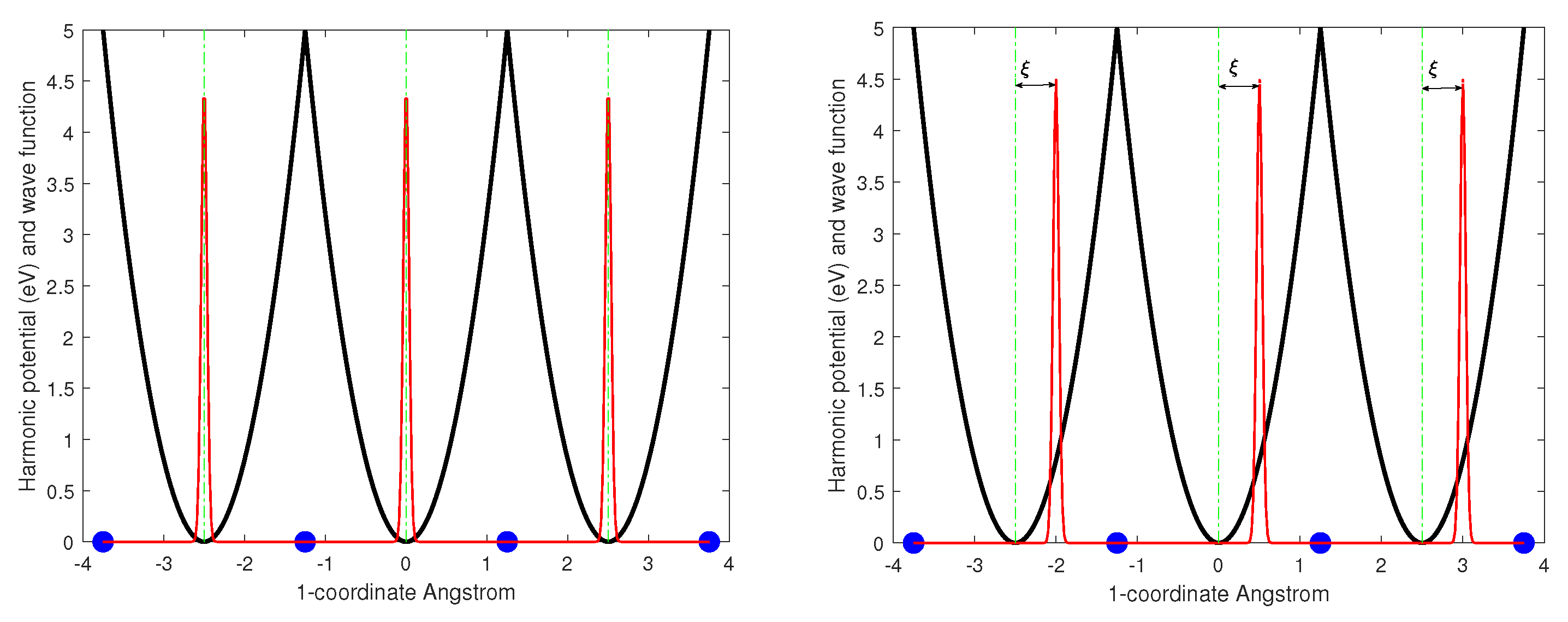
Let us consider a system of charged identical quantum oscillators placed at the vertices of a simple cubic three-dimensional lattice with spacing d. Here, we suppose that the oscillator n is in its equilibrium position at site n of the lattice, meaning that there are N oscillators in a lattice with N elementary cells (Figure 1). Oscillator n is kept in its equilibrium position by a potential $V_n({\overrightarrow{\xi }}_n)$, which is harmonic with frequency $\omega$ when $|{\overrightarrow{\xi }}_n|$ is small enough and becomes stiffer when the oscillation approaches the boundary of the elementary cell. This requirement guarantees that the oscillation does not interfere with the adjacent elementary cells and remains confined in the nth cell.

The Hamiltonian of the single harmonic oscillator is as follows (we use natural units with $\hslash =c=k_B={\epsilon }_0=1$):

$$H_{\mathrm{osc}}^{\left(1\right)}=\frac{{[\overrightarrow{p}+e\overrightarrow{A}(\overrightarrow{\xi },t)]}^2}{2m}+\frac{m{\omega }^2}{2}{\overrightarrow{\xi }}^2$$

(1)

where e, m, and $\omega$ are the charge, mass, and oscillation frequency of the oscillator at position $\overrightarrow{\xi }$, while $\overrightarrow{A}(\overrightarrow{\xi },t)$ is the electromagnetic vector potential.

Due to the self-generated electrostatic interaction, the particles experience an additional potential provided by $V_p\left(\overrightarrow{\xi }\right)=\frac{m{\omega }_p^2}{2}{\overrightarrow{\xi }}^2$, where ${\omega }_p=\sqrt{\frac{e^{2}N}{mV}}$ is the free plasma frequency.

Therefore, the total Hamiltonian describing the oscillators in interaction with the electromagnetic field is

$$H_{\mathrm{osc}}^{\left(N\right)}=\sum _{n=1}^N\frac{{[{\overrightarrow{p}}_n+e\overrightarrow{A}({\overrightarrow{x}}_n+{\overrightarrow{\xi }}_n,t)]}^2}{2m}+\frac{m({\omega }^2+{\omega }_p^2)}{2}{\overrightarrow{\xi }}_n^2$$

(2)

where ${\overrightarrow{x}}_n$ is the equilibrium position of the nth oscillator.

By adding to (2) the free electromagnetic Hamiltonian, the total Hamiltonian can be rewritten in second-quantized terms as

$${\widehat{H}}_{\mathrm{tot}}=\widehat{H}+{\widehat{H}}_{\mathrm{int}}+{\widehat{H}}_{\mathrm{photon}}$$

(3)

where

$$\begin{array}{cc}\hfill \widehat{H}=& {\omega }^{\prime }\sum _{n=1}^N\left[{\overrightarrow{a}}_n^{†}\left(t\right)·{\overrightarrow{a}}_n\left(t\right)+\frac{3}{2}\right]\hfill \end{array}$$

(4a)

$$\begin{array}{cc}\hfill {\widehat{H}}_{\mathrm{int}}=& \sum _{n=1}^N\frac{e}{m}{\widehat{\overrightarrow{p}}}_n·\widehat{\overrightarrow{A}}({\overrightarrow{x}}_n+{\overrightarrow{\xi }}_n,t)\hfill \end{array}$$

(4b)

$$\begin{array}{cc}\hfill {\widehat{H}}_{\mathrm{photon}}=& \omega \sum _{p=1}^2\int d{\mathrm{\Omega }}_{\widehat{k}}\left[b_{p,\overrightarrow{k}}^{†}\left(t\right)b_{p,\overrightarrow{k}}\left(t\right)+\frac{1}{2}\right]+\sum _{n=1}^N\frac{e^2}{2m}{\widehat{\overrightarrow{A}}}^2({\overrightarrow{x}}_n+{\overrightarrow{\xi }}_n,t)\hfill \end{array}$$

(4c)

and where we have defined the shifted oscillation frequency as

$${\omega }^{\prime }=\sqrt{{\omega }^2+{\omega }_p^2}.$$

(5)

Note that for the electromagnetic field we have selected the modes with frequency $\omega$ only, as we are interested in the modes that have a relevant dynamical impact on the system under study in a way that becomes clear in the following. The neglected modes interact with the system only perturbatively.

The destruction and creation operators $a_n\left(t\right)$, $a_n^{†}\left(t\right)$, $b_{p,\overrightarrow{k}}\left(t\right)$ and $b_{p,\overrightarrow{k}}^{†}\left(t\right)$ are in the interaction picture, meaning that

$$\left\{\begin{array}{cc}\hfill a_n\left(t\right)=& a_n{e}^{-i{\omega }^{\prime }t}\hfill \\ \hfill a_n^{†}\left(t\right)=& a_n^{†}{e}^{i{\omega }^{\prime }t}\hfill \\ \hfill b_{p,\overrightarrow{k}}\left(t\right)=& b_{p,\overrightarrow{k}}{e}^{-i\omega t}\hfill \\ \hfill b_{p,\overrightarrow{k}}^{†}\left(t\right)=& b_{p,\overrightarrow{k}}^{†}{e}^{i\omega t}\hfill \end{array}\right.$$

(6)

and the radiation field operator is given by

$$\widehat{\overrightarrow{A}}(\overrightarrow{x},t)=\frac{1}{\sqrt{2\omega V}}\sum _{p=1}^2\int d{\mathrm{\Omega }}_{\widehat{k}}[b_{p,\overrightarrow{k}}\left(t\right)e^{i\overrightarrow{k}·\overrightarrow{x}}{\overrightarrow{\epsilon }}_{p,\overrightarrow{k}}+b_{p,\overrightarrow{k}}^{†}\left(t\right)e^{-i\overrightarrow{k}·\overrightarrow{x}}{\overrightarrow{\epsilon }}_{p,\overrightarrow{k}}^{*}]$$

(7)

where $|\overrightarrow{k}|=\omega$, ${\overrightarrow{\epsilon }}_{p,\overrightarrow{k}}·\overrightarrow{k}=0$ and ${\overrightarrow{\epsilon }}_{p,\overrightarrow{k}}^{*}·{\overrightarrow{\epsilon }}_{p^{\prime },\widehat{k}}={\delta }_{p{p}^{\prime }}$. Here p is a polarization index and the e.m. wave unit vector $\widehat{k}=\overrightarrow{k}/\omega$ spans all possible 3D directions. In order to get rid of the diamagnetic term $\frac{e^2}{2m}{\sum }_{n=1}^N{\widehat{\overrightarrow{A}}}^2({\overrightarrow{\xi }}_n,t)$ we will proceed in the context of the dipole approximation. Following the lines described in Appendix B [9], we can recast Equation (4c) in terms of new photon operators so that

$${\widehat{H}}_{\mathrm{photon}}={\omega }^{\prime }\sum _{p=1}^2\int d{\mathrm{\Omega }}_{\widehat{k}}\left(c_{p,\overrightarrow{k}}^{†}{c}_{p,\overrightarrow{k}}+\frac{1}{2}\right).$$

(8)

Equation (8) shows that the transformation (A14) makes the diamagnetic term disappear, making the electromagnetic Hamiltonian diagonal. The oscillation frequency is shifted to the new value ${\omega }^{\prime }$, equal to that of the matter field. Moreover, the electromagnetic modes acquire a mass and their dispersion relation is modified such that the electromagnetic field is not able to propagate through the vacuum and cannot escape from the material.

The last term of the Hamiltonian can now be written in terms of the new operators. By means of the canonical transformations

$$\begin{array}{cc}\hfill \overrightarrow{a}=& \frac{1}{\sqrt{2}}\left(\frac{1}{{\xi }^{\prime }}\overrightarrow{\xi }+i{\xi }^{\prime }\overrightarrow{p}\right)\hfill \\ \hfill {\overrightarrow{a}}^{†}=& \frac{1}{\sqrt{2}}\left(\frac{1}{{\xi }^{\prime }}\overrightarrow{\xi }-i{\xi }^{\prime }\overrightarrow{p}\right)\hfill \end{array}$$

(9)

and

$$\begin{array}{cc}\hfill \overrightarrow{\xi }=& {\xi }^{\prime }\frac{\overrightarrow{a}+{\overrightarrow{a}}^{†}}{\sqrt{2}}\hfill \\ \hfill \overrightarrow{p}=& \frac{i}{{\xi }^{\prime }}\frac{{\overrightarrow{a}}^{†}-\overrightarrow{a}}{\sqrt{2}}\hfill \end{array}$$

(10)

where we have defined ${\xi }^{\prime }={\left(m{\omega }^{\prime }\right)}^{-\frac{1}{2}}$, we can recast Equation (4b) as

$${\widehat{H}}_{\mathrm{int}}=\frac{e}{m}\frac{1}{\sqrt{2{\omega }^{\prime }V}}\frac{i}{{\xi }^{\prime }}\sum _{n=1}^N\frac{{\overrightarrow{a}}_n^{†}\left(t\right)-{\overrightarrow{a}}_n\left(t\right)}{\sqrt{2}}·\sum _{p=1}^2\int d{\mathrm{\Omega }}_{\widehat{k}}[c_{p,\overrightarrow{k}}\left(t\right)e^{i\overrightarrow{k}·\overrightarrow{x}}{\overrightarrow{\epsilon }}_{p,\overrightarrow{k}}+c_{p,\overrightarrow{k}}^{†}\left(t\right)e^{-i\overrightarrow{k}·\overrightarrow{x}}{\overrightarrow{\epsilon }}_{p,\overrightarrow{k}}^{*}]$$

(11)

Because we are considering e.m. modes for which the wavelength is much larger than the lattice constant, we may neglect the spatial dependence of the electromagnetic field (dipole approximation, DA); thus, Equation (11) becomes

$${\widehat{H}}_{\mathrm{int}}=\frac{i{\omega }_p}{2\sqrt{N}}\sum _{n=1}^N({\overrightarrow{a}}_n^{†}\left(t\right)-{\overrightarrow{a}}_n\left(t\right))·\sum _{p=1}^2\int d{\mathrm{\Omega }}_{\widehat{k}}[c_{p,\overrightarrow{k}}\left(t\right){\overrightarrow{\epsilon }}_{p,\overrightarrow{k}}+c_{p,\overrightarrow{k}}^{†}\left(t\right){\overrightarrow{\epsilon }}_{p,\overrightarrow{k}}^{*}]$$

(12)

where the coupling strength turns out to be proportional to the plasma frequency ${\omega }_p$.

In the next section, we proceed through a variational calculation of the minimum energy of the dynamical system described by Equations (4a), (8), and (12) when probed by coherent matter–photon states.

3. Selection of the Quantum State for the Electromagnetic Field

The modes of the electromagnetic field that are eligible for resonant interaction with the oscillators are those with frequencies that equal $\omega$, more precisely, those selected in Equation (12). The number of such independent modes is $2·4\pi$, distributed along the possible directions of the electromagnetic momentum $\omega \widehat{k}$ and the electric polarization. We note here that we are now diverging from the usual treatment of the electromagnetic field in resonant cavities, as our analysis is not limited to the wave vectors in a single direction; rather, we consider the contribution of all the wave vectors with moduli $|\overrightarrow{k}|=\omega$. This fact is bound to have dramatic consequences on the final result.

Assuming, without loss of generality, that the oscillation of the charges is along the direction $\widehat{1}$, we can define the photon states

$$|{\omega }^{\prime },\widehat{1}\rangle =\sqrt{\frac{3}{8\pi }}\sum _{p=1}^2\int d{\mathrm{\Omega }}_{\widehat{k}}\langle \widehat{1}|{\overrightarrow{\epsilon }}_{p,\overrightarrow{k}}\rangle |\overrightarrow{k},p\rangle$$

(13)

where the integral is performed over the directions of the unit vector $\widehat{k}$. These states are properly normalized thanks to the relation

$$\sum _{p=1}^2\int d{\mathrm{\Omega }}_{\widehat{k}}{\left|\langle \widehat{1}|{\overrightarrow{\epsilon }}_{p,\overrightarrow{k}}\rangle \right|}^2=\int d{\mathrm{\Omega }}_{\widehat{k}}\langle \widehat{1}|[\mathbb{1}-|\widehat{k}\rangle \langle \widehat{k}|]|\widehat{1}\rangle =4\pi -\int d{\mathrm{\Omega }}_{\widehat{k}}{cos}^2{\theta }_{\widehat{k}}=\frac{8\pi }{3}.$$

(14)

The states $|{\omega }^{\prime },\widehat{1}\rangle$ are created and annihilated by the operators

$$\{\begin{array}{}\mathrm{(15a)}& C_1^{†}=\sqrt{\frac{3}{8\pi }}{\displaystyle \sum _{p=1}^2}\int d{\mathrm{\Omega }}_{\widehat{k}}{\langle \widehat{1}|{\overrightarrow{\epsilon }}_{p,\overrightarrow{k}}\rangle }^{*}{c}_{\overrightarrow{k},p}^{†}\mathrm{(15b)}& C_1=\sqrt{\frac{3}{8\pi }}{\displaystyle \sum _{p=1}^2}\int d{\mathrm{\Omega }}_{\widehat{k}}\langle \widehat{1}|{\overrightarrow{\epsilon }}_{p,\overrightarrow{k}}\rangle c_{\overrightarrow{k},p}.\end{array}$$

By introducing the operators

$$\{\begin{array}{}\mathrm{(16a)}& C_2^{†}=\sqrt{\frac{3}{8\pi }}{\displaystyle \sum _{p=1}^2}\int d{\mathrm{\Omega }}_{\widehat{k}}{\langle \widehat{2}|{\overrightarrow{\epsilon }}_{p,\overrightarrow{k}}\rangle }^{*}{c}_{\overrightarrow{k},p}^{†}\mathrm{(16b)}& C_2=\sqrt{\frac{3}{8\pi }}{\displaystyle \sum _{p=1}^2}\int d{\mathrm{\Omega }}_{\widehat{k}}\langle \widehat{2}|{\overrightarrow{\epsilon }}_{p,\overrightarrow{k}}\rangle c_{\overrightarrow{k},p}\mathrm{(16c)}& C_3^{†}=\sqrt{\frac{3}{8\pi }}{\displaystyle \sum _{p=1}^2}\int d{\mathrm{\Omega }}_{\widehat{k}}{\langle \widehat{3}|{\overrightarrow{\epsilon }}_{p,\overrightarrow{k}}\rangle }^{*}{c}_{\overrightarrow{k},p}^{†}\mathrm{(16d)}& C_3=\sqrt{\frac{3}{8\pi }}{\displaystyle \sum _{p=1}^2}\int d{\mathrm{\Omega }}_{\widehat{k}}\langle \widehat{3}|{\overrightarrow{\epsilon }}_{p,\overrightarrow{k}}\rangle c_{\overrightarrow{k},p}\end{array}$$

the commutation relations for the new operators are

$$[C_i,C_j^{†}]=\frac{3}{8\pi }\sum _{p=1}^2\int d{\mathrm{\Omega }}_{\widehat{k}}\langle \widehat{i}|{\overrightarrow{\epsilon }}_{p,\overrightarrow{k}}\rangle \langle {\overrightarrow{\epsilon }}_{p,\overrightarrow{k}}|\widehat{j}\rangle ={\delta }_{ij},[C_i^{†},C_j^{†}]=[C_i,C_j]=0$$

(17)

meaning that Equations (15) and (16) are canonical transformations. The vector potential after the DA can be rewritten in terms of these operators as

$$\widehat{\overrightarrow{A}}=\frac{1}{\sqrt{2{\omega }^{\prime }V}}\left[(C_1+C_1^{†})\widehat{1}+(C_2+C_2^{†})\widehat{2}+(C_3+C_3^{†})\widehat{3}\right].$$

(18)

We can now express the interaction and photon Hamiltonians in terms of the new operators. Immediately, from Equation (12) we obtain

$${\widehat{H}}_{\mathrm{int}}=\frac{i{\omega }_p}{2\sqrt{N}}\sqrt{\frac{8\pi }{3}}\sum _{n=1}^N[a_{1,n}^{†}{C}_1-a_{1,n}{C}_1^{†}+a_{1,n}^{†}{C}_1^{†}-a_{1,n}{C}_1]$$

(19)

and from Equation (8) we obtain

$$\begin{array}{cc}\hfill {\widehat{H}}_{\mathrm{photon}}=& {\omega }^{\prime }{\displaystyle \sum _{i=1}^3}\left[C_i^{†}{C}_i+\frac{1}{2}\right]\hfill \end{array}$$

(20)

Equations (19) and (20) tell us that the different modes of the electromagnetic field contribute to an increase in the coupling with the matter field, and such an interaction does not affect the energy density of the electromagnetic field. It will be seen in the next sections how this fact avoids the no-go theorem [2,10] while leading to the instability of the perturbative vacuum and to the migration of the field to a new stable and coherent configuration.

4. Effective Hamiltonian

Let us consider the trial coherent state

$$|\mathrm{\Omega }\rangle =\underset{i=1\dots 3;n}{⨂}{|{\alpha }_i\rangle }_n\underset{j=1\dots 3}{⨂}|{\mathcal{A}}_j\rangle$$

(21)

with the definitions

$$\begin{array}{cc}\hfill {|{\alpha }_i\rangle }_n=& e^{-\frac{1}{2}{\left|{\alpha }_i\right|}^2}\sum _{m=0}^{\infty }\frac{{\alpha }_i^m}{m!}{a}_{i,n}^{†m}{|0\rangle }_n\hfill \end{array}$$

(22a)

$$\begin{array}{cc}\hfill |{\mathcal{A}}_j\rangle =& e^{-\frac{1}{2}N{\left|{\mathcal{A}}_j\right|}^2}\sum _{p=0}^{\infty }\frac{{\left(\sqrt{N}{\mathcal{A}}_j\right)}^p}{p!}{C}_j^{†p}|0\rangle .\hfill \end{array}$$

(22b)

The state $|\mathrm{\Omega }\rangle$ is a coherent state with a vector order parameter $\overrightarrow{\alpha }$ for the matter sector and $\sqrt{N}\overrightarrow{\mathcal{A}}$ for the electromagnetic sector. We make a further choice in setting ${\alpha }_2={\alpha }_3={\mathcal{A}}_2={\mathcal{A}}_3=0$ such that

$$\begin{array}{cc}\hfill {\overrightarrow{a}}_n|\mathrm{\Omega }\rangle =& \widehat{1}\alpha |\mathrm{\Omega }\rangle \hfill \end{array}$$

(23a)

$$\begin{array}{cc}\hfill \overrightarrow{C}|\mathrm{\Omega }\rangle =& \sqrt{N}\widehat{1}\mathcal{A}|\mathrm{\Omega }\rangle \hfill \end{array}$$

(23b)

The two order parameters $\alpha \left(t\right)$ and $\mathcal{A}\left(t\right)$ are complex functions that are treated as both variational parameters and as the solution of the emerging dynamical equations. The all-important feature of the state $|\mathrm{\Omega }\rangle$ is that the parameter $\alpha$ is the same for all n, allowing us to drop the index n from the operators such that Equations (4a), (12), and (20) can be rewritten as

$$\begin{array}{cc}\hfill \langle \mathrm{\Omega }|H|\mathrm{\Omega }\rangle =& N{\omega }^{\prime }\left[{\left|\alpha \right|}^2+\frac{3}{2}\right]\hfill \end{array}$$

(24a)

$$\begin{array}{cc}\hfill \langle \mathrm{\Omega }|H_{\mathrm{int}}|\mathrm{\Omega }\rangle =& \frac{i{\omega }_{p}N}{2}\sqrt{\frac{8\pi }{3}}[{\alpha }^{*}\mathcal{A}-\alpha {\mathcal{A}}^{*}+{\alpha }^{*}{\mathcal{A}}^{*}-\alpha \mathcal{A}]\hfill \end{array}$$

(24b)

$$\begin{array}{cc}\hfill \langle \mathrm{\Omega }|H_{\mathrm{photon}}|\mathrm{\Omega }\rangle =& {\omega }^{\prime }\left[{N\left|\mathcal{A}\right|}^2+\frac{3}{2}\right].\hfill \end{array}$$

(24c)

Equation (24) lead to the Schrödinger-like equation

$$\langle \mathrm{\Omega }|i\frac{\partial }{\partial t}|\mathrm{\Omega }\rangle =\langle \mathrm{\Omega }|H_{\mathrm{tot}}|\mathrm{\Omega }\rangle .$$

(25)

By setting $\alpha \left(t\right)=\left|\alpha \right|e^{-i\tilde{\omega }t}$, $\mathcal{A}\left(t\right)=\left|\mathcal{A}\right|e^{-i(\tilde{\omega }t-\frac{\pi }{2})}$ and $\epsilon =\frac{{\omega }_p}{{\omega }^{\prime }}$, Equation (24) add up to

$${\langle \mathrm{\Omega }|H_{\mathrm{tot}}|\mathrm{\Omega }\rangle }^{\left(1\right)}=N{\omega }^{\prime }\left[{\left|\alpha \right|}^2+\frac{3}{2}-\sqrt{\frac{8\pi }{3}}\epsilon \left|\alpha \mathcal{A}\right|+{\left|\mathcal{A}\right|}^2+\frac{3}{2N}\right]+{\mathcal{H}}_{crt}\left(t\right),$$

(26)

where

$${\mathcal{H}}_{crt}\left(t\right)=N{\omega }^{\prime }\sqrt{\frac{2\pi }{3}}\epsilon \left|\alpha \mathcal{A}\right|(e^{2i\tilde{\omega }t}+e^{-2i\tilde{\omega }t})$$

(27)

are the counter-rotating terms that wildly oscillate at the double of the frequency $\tilde{\omega }$ and where the superscript ${}^{\left(1\right)}$ indicates that the calculation is at first order in perturbation theory.

We now introduce the rotating wave approximation (RWA), consisting in neglecting the term ${\mathcal{H}}_{crt}\left(t\right)$ in the effective Hamiltonian. We note that the counter-rotating terms of the type $ab$ and $a^{†}{b}^{†}$, after being evaluated on the trial state, produce terms proportional to $A\left(t\right)\alpha \left(t\right)$ and $A^{*}\left(t\right){\alpha }^{*}\left(t\right)$ which have a time dependence of the type $exp(\pm 2i\tilde{\omega }t)$ and are averaged to zero over an oscillation period. This does not happen for the retained terms, which have a temporal dependence of type $A^{*}\left(t\right)\alpha \left(t\right)$ and $A\left(t\right){\alpha }^{*}\left(t\right)$. They are time-independent, and as such are the only ones that make a contribution to the trial state’s energy. For this reason, it is legitimate to apply the RWA approximation in our calculation, even though it is generally not valid in cavity QED in the presence of ultra-strong coupling [26].

Equation (25) then leads to

$$\tilde{\omega }=N{\omega }^{\prime }\left[{\left|\alpha \right|}^2+\frac{3}{2}-\sqrt{\frac{8\pi }{3}}\epsilon \left|\alpha \mathcal{A}\right|+{\left|\mathcal{A}\right|}^2+\frac{3}{2N}\right].$$

(28)

We are now equipped with a set of legitimate matter–field quantum states that satisfy the dynamical equations depending parametrically on $\left|\alpha \right|$ and $\left|\mathcal{A}\right|$. Our goal is to look for solutions with energy contents lower than that of the perturbative vacuum $\left|\alpha \right|=\left|\mathcal{A}\right|=0$. To this end, we define the energy gap per particle as $\delta E_{\mathrm{\Omega }}^{\left(1\right)}=\frac{1}{N}{\langle \mathrm{\Omega }|H_{\mathrm{tot}}|\mathrm{\Omega }\rangle }^{\left(1\right)}-{\omega }^{\prime }\left[\frac{3}{2}+\frac{3}{2N}\right]$ and find the minimum with respect to the parameter $\left|\mathcal{A}\right|$ by requiring

$$\frac{\partial \delta E_{\mathrm{\Omega }}^{\left(1\right)}}{\partial \left|\mathcal{A}\right|}=0.$$

(29)

The minimum is found for $\left|\mathcal{A}\right|=\sqrt{\frac{2\pi }{3}}\left|\alpha \right|$, and the minimum of the energy gap is

$$\delta E_{\mathrm{\Omega }}^{\left(1\right)}={\omega }^{\prime }{\left|\alpha \right|}^2\left(1-\frac{2\pi }{3}{\epsilon }^2\right).$$

(30)

Equation (30) shows that the vacuum becomes unstable when

$$\epsilon >{\epsilon }_{\mathrm{crit}}=\sqrt{\frac{3}{2\pi }}\simeq 0.69,$$

(31)

which is well within the allowed range $0<\epsilon <1$.

This result reveals the existence of a phase transition to a new vacuum of the system. However, when looking at Equation (30) it appears that the new vacuum has a negatively diverging gap due to the freedom of the variational parameter $\left|\alpha \right|$, which is clearly a non-physical situation. Fortunately, due to the intervention of other factors not considered in the Hamiltonian that limit the oscillations of the charges outside their reticular cages, the parameter $\left|\alpha \right|$ cannot assume arbitrarily large values, making the result of Equation (30) meaningful and rich of physical consequences.

To be more specific, we must consider that the Hamiltonian (4a) is a quadratic approximation of the true Hamiltonian that is valid for small oscillations around the equilibrium positions of the oscillating charges and fails when the oscillation amplitude exceeds a certain value. The complete Hamiltonian contains terms that prevent the oscillations from exceeding the dimensions of the reticular cage. The detailed form of such terms is unknown, as it depends on the details of the charge distributions of the host lattice. Here, we introduce the effect of these terms by imposing a maximum value on the amplitude of oscillation of the charges, which is fixed by the size and shape of the lattice cells. We address these topics in the following paragraphs.

It is important to note that symmetry-breaking of the vacuum is made possible by the synergistic cooperation of the various modes of the electromagnetic field, which make the coupling to the matter field $\sqrt{\frac{8\pi }{3}}$ times that of the single mode (Equation (19)). As far as we know, to date this feature represents a novelty in the literature dedicated to the study of the strong coupling regime. Had we only considered the two polarization modes and the two directions $\widehat{k}$ and $-\widehat{k}$ along a fixed axis of the field, we would not have obtained sufficiently intense coupling with the matter to induce the transition. In fact, the factor $\sqrt{\frac{8\pi }{3}}$ would have been substituted by $\sqrt{2·2}$ (provided by the two polarizations and the two directions), and Equation (30) would have been substituted by the similar equation

$$\delta E_{\mathrm{\Omega }}^{\left(1\right)}={\omega }^{\prime }{\left|\alpha \right|}^2\left(1-{\epsilon }^2\right),$$

(32)

which displays no instability for $\epsilon$ in the allowed range $(0,1)$ and reproduces the result of various no-go theorems in the literature [2,10]. It is therefore imperative to consider the photon state (13) in order to achieve symmetry-breaking.

5. Lower Bound of the Energy Gap for the Coherent Phase

When condition (31) is met, Equation (30) is unbounded from below because $\left|\alpha \right|$ can assume any value, which is an obviously non-physical condition. Little thought is required to spot the direction we need to take in order to recover a physically sound result; the parameter $\left|\alpha \right|$ is related to the maximum amplitude of the plasma oscillation of the charges, and it is clear that such an oscillation cannot take arbitrarily large values because it is limited by the linear size of the lattice “cages” with spacing d. Mathematically, this may be formulated by introducing anharmonic terms into the matter Hamiltonian that are negligible for small plasma oscillations and become predominant when the oscillation exceeds the cage dimension. To implement this condition, we need to fix a maximum value of the oscillation amplitude of the matter field, which in general is provided by a fraction f of the linear dimension d of the electrostatic cages. Indeed, using Equation (10) we must have

$$\frac{{{\xi }^{\prime }}^2}{2}\underset{t}{max}\langle \mathrm{\Omega }|{(a_n\left(t\right)+a_n^{†}\left(t\right))}^2|\mathrm{\Omega }\rangle =\frac{f^2{d}^2}{4}$$

(33)

which, recalling Equation (23a), becomes

$${\left|\alpha \right|}^2=\frac{f^2{d}^2}{8{{\xi }^{\prime }}^2}-\frac{1}{4}=\frac{m{f}^2{d}^2{\omega }^{\prime }}{8}-\frac{1}{4}$$

(34)

In all practical situations, the last term in Equation (34) stemming from the indetermination principle can be neglected (being $d^{2}m{\omega }^{\prime }>>2$) and the energy gap per particle has the form

$$\delta E_{\mathrm{\Omega }}^{\left(1\right)}=\frac{m{f}^2{d}^2{{\omega }^{\prime }}^2}{8}\left(1-\frac{2\pi }{3}{\epsilon }^2\right).$$

(35)

It is important to note that, had we used plane wave functions in place of coherent states, we would not have been able to use any arguments relating to the non-divergence of the energy gap, obliging us to declare the resulting solutions to be non-physical.

To summarize this section, we have found that when an ensemble of charged particles embedded in a neutralizing charge density of opposite charges reaches a critical density, it is subjected to a spontaneous quantum phase transition to a stable, collective, and coherent state that is strongly and resonantly coupled to a coherent electromagnetic field with a total energy lower than that of the incoherent state (i.e., uncorrelated particles and no macroscopic electromagnetic field) by a finite amount.

This configuration involves a very large number of particles and has a spatial extension much larger than the typical atomic radius. In Section 8, we estimate the spatial structure and introduce the key concept of coherence domain (CD).

6. Second-Order Perturbation Theory for Composite Coherent States

We now proceed with the analysis of the energy content of the trial state (21) by studying the second order contribution of the perturbative expansion of the ground state energy. In physical terms, the first order contribution takes into account the contribution to the energy of the photons emitted by the oscillators and reabsorbed by the same oscillators, whereas the second order contribution considers the dispersive contribution of photons emitted by an oscillator and absorbed by a different oscillator. As we show below, it turns out that the two terms contribute the same amount, thereby doubling the term of negative interaction and strengthening the condensation mechanism.

To apply the second order perturbation theory, we need an orthonormal basis over which we can expand our trial state. To this end, we use the property of the interaction term $H_{\mathrm{int}}$ to preserve the sum of the number of photons and the excitation number of the oscillators (the creation of a photon involves the reduction of the excitation state of the oscillator and vice versa), then define the new normalized basis as

$${|\sigma ,\alpha ,\mathcal{A}\rangle }_n=\frac{\sqrt{\sigma !}}{R^{\sigma }}\sum _{\eta =0}^{\sigma }\frac{{\alpha }^{\sigma -\eta }}{\sqrt{(\sigma -\eta )!}}\frac{N^{\eta /2}{\mathcal{A}}^{\eta }}{\sqrt{\eta !}}{|\sigma -\eta \rangle }_n\otimes |\eta \rangle$$

(36)

where we have defined $R=\sqrt{{\left|\alpha \right|}^2+N{\left|\mathcal{A}\right|}^2}$ such that the trial state can be rewritten as

$$|\mathrm{\Omega }\rangle =e^{-\frac{1}{2}{R}^2}\sum _{\sigma =0}^{\infty }\frac{R^{\sigma }}{\sqrt{\sigma !}}\underset{n}{⨂}{|\sigma ,\alpha ,\mathcal{A}\rangle }_n.$$

(37)

The properties of the states ${|\sigma ,\alpha ,\mathcal{A}\rangle }_n$ are as follows:

• ${}_n\langle \sigma ,\alpha ,\mathcal{A}|{\sigma }^{\prime },\alpha ,\mathcal{A}\rangle {}_{n^{\prime }}={\delta }_{\sigma {\sigma }^{\prime }}{\delta }_{n{n}^{\prime }}$
• The expectation value of $H_{\mathrm{int}}$ (Equation (19)) on the states ${|\sigma ,\alpha ,\mathcal{A}\rangle }_n$ (see Appendix C) is provided by

  $${}_n\langle \sigma ,\alpha ,\mathcal{A}|H_{\mathrm{int}}|{\sigma }^{\prime },\alpha ,\mathcal{A}\rangle {}_{n^{\prime }}=-{\omega }_p\sqrt{\frac{8\pi }{3}}\left|\alpha \mathcal{A}\right|\frac{\sigma }{R^2}{\delta }_{\sigma {\sigma }^{\prime }}{\delta }_{n{n}^{\prime }}$$

  (38)
• The expectation value of the unperturbed Hamiltonian (see Appendix C) is

  $$\langle \sigma ,\alpha ,\mathcal{A}|H+{\widehat{H}}_{\mathrm{photon}}|\sigma ,\alpha ,\mathcal{A}\rangle ={\omega }^{\prime }\left[N\left(\sigma \frac{{\left|\alpha \right|}^2}{R^2}+\frac{3}{2}+{\left|\mathcal{A}\right|}^2\frac{\sigma }{R^2}\right)+\frac{3}{2}\right]$$

  (39)

We are now ready to compute the second-order contribution to the energy.

7. The Second-Order Contribution

We start from the well-known second order perturbation theory in the Brillouin–Wigner approximation [27]:

$$E_{\sigma }=h_{0p}+h_1+\frac{h_1^2}{E_{\sigma }-(h_{0p}+h_1)}$$

(40)

where, for simplicity, we have indicated $|\sigma \rangle ={⨂}_n{|\sigma ,\alpha ,\mathcal{A}\rangle }_n$, $h_{0p}=\langle \sigma |H+{\widehat{H}}_{\mathrm{photon}}|\sigma \rangle$ and $h_1=\langle \sigma |H_{\mathrm{int}}|\sigma \rangle$.

Strictly speaking, the numerator of Equation (40) should be $\frac{N(N-1)}{N^2}{h}_1^2$, as the sum over the unperturbed states should exclude the diagonal terms; however, as N is very large, here we may set $N(N-1)/N^2\simeq 1$.

The solutions of Equation (40) are

$$E_{\sigma }=h_{0p}+(1\pm 1)h_1$$

(41)

and the lowest energy per particle of the states $|\sigma \rangle$ is $E_{\sigma }=h_{0p}+2h_1$. Substitution of Equations (38) and (39) into Equation (3) at the second order yields

$$\begin{array}{cc}\hfill \frac{1}{N}{\langle \mathrm{\Omega }|H_{\mathrm{tot}}|\mathrm{\Omega }\rangle }^{\left(2\right)}& =e^{-R^2}\sum _{\sigma =0}^{\infty }\frac{R^{2\sigma }}{\sigma !}\frac{E_{\sigma }}{N}=\hfill \\ & ={\omega }^{\prime }\left[{\left|\alpha \right|}^2+\frac{3}{2}+\frac{3}{2N}-\sqrt{\frac{8\pi }{3}}2\epsilon \left|\alpha \mathcal{A}\right|+{\left|\mathcal{A}\right|}^2\right].\hfill \end{array}$$

(42)

Equation (42) shows that at the second order the contribution of the negative interaction term is twice the contribution at the first order, meaning that the coupling threshold is further lowered compared to the first order calculation. By repeating the procedure already performed in Section 4, we find

$$\begin{array}{cc}\hfill \left|\mathcal{A}\right|=& \sqrt{\frac{8\pi }{3}}\left|\alpha \right|\hfill \end{array}$$

(43a)

$$\begin{array}{cc}\hfill \delta E_{\mathrm{\Omega }}^{\left(2\right)}=& \frac{m{f}^2{d}^2{{\omega }^{\prime }}^2}{8}\left(1-\frac{8\pi }{3}{\epsilon }^2\right).\hfill \end{array}$$

(43b)

$$\begin{array}{cc}\hfill {\epsilon }_{\mathrm{crit}}^{\left(2\right)}=& \sqrt{\frac{3}{8\pi }}\simeq 0.35\hfill \end{array}$$

(43c)

As anticipated at the beginning of Section 6, the threshold for the onset of coherence is significantly lowered and the energy gap is more pronounced compared to the calculation at first order.

8. Spatial Dimension of the Coherent States and Concept of Natural Resonating Cavity

We have shown that the dynamical relevance of quantum states is composed of a very large number of elementary charged particles plus a macroscopic (classical) electromagnetic field with an energy content lower than that of the perturbative state.

The properties of the coherent state (21) allow us to identify two vector order parameters, $\overrightarrow{\alpha }\left(t\right)$ and $\overrightarrow{\mathcal{A}}\left(t\right)$, for which the temporal evolution is

$$\begin{array}{cc}\hfill \overrightarrow{\alpha }\left(t\right)=& \left[\begin{array}{ccc}\alpha & 0& 0\end{array}\right]e^{-i\tilde{\omega }t}\hfill \end{array}$$

(44a)

$$\begin{array}{cc}\hfill \overrightarrow{\mathcal{A}}\left(t\right)=& \left[\begin{array}{ccc}\mathcal{A}& 0& 0\end{array}\right]e^{i(\frac{\pi }{2}-\tilde{\omega }t)}\hfill \end{array}$$

(44b)

where $\alpha \ge 0$ and $\mathcal{A}\ge 0$. The choice of a spatial direction of 1 is arbitrary.

Thus far, we have neglected the spatial properties of the problem. The reason for this is the very long wavelength of the radiation field compared to the scale of the lattice. We now wish to obtain more insight into the nature of the spatial properties of the lowest-energy state. The wave number of the radiation field is unaffected by the coherent transition, and is provided by

$$|\overrightarrow{k}|=\omega =\sqrt{{{\omega }^{\prime }}^2-{\omega }_p^2}=\frac{2\pi }{\lambda }$$

(45)

where it is reasonable to expect that the spatial region in which a coherent condensation can occur has a minimum radius on the order of the half-wavelength $r_{CD}=\lambda /2=\frac{\pi }{\omega }$. We refer to this region as the coherence domain (CD).

Returning to the definition of the photon field (7), we can reformulate the expansion in plane waves in terms of spherical harmonics provided by [28]

$$e^{i\overrightarrow{k}·\overrightarrow{x}}=4\pi \sum _{\genfrac{}{}{0pt}{}{l=0}{\left|m\right|\le l}}^{\infty }{i}^l{j}_l\left(\right|\overrightarrow{k}\left|\right|\overrightarrow{x}\left|\right)Y_{lm}^{*}\left(\widehat{k}\right)Y_{lm}\left(\widehat{x}\right).$$

(46)

By substitution, we obtain

$$\widehat{\overrightarrow{A}}(\overrightarrow{x},t)={\widehat{\overrightarrow{A}}}_0(\overrightarrow{x},t)+\delta \widehat{\overrightarrow{A}}(\overrightarrow{x},t)$$

(47)

where

$$\begin{array}{cc}\hfill {\widehat{\overrightarrow{A}}}_0(\overrightarrow{x},t)=& \frac{j_0\left(\omega r\right)}{\sqrt{2{\omega }^{\prime }V}}\sum _{z=1}^3(C_z+C_z^{†})\widehat{z}\hfill \end{array}$$

(48a)

$$\begin{array}{cc}\hfill \delta \widehat{\overrightarrow{A}}(\overrightarrow{x},t)=& \sum _{\genfrac{}{}{0pt}{}{l=1}{\left|m\right|\le l}}^{\infty }\frac{4\pi j_l\left(\omega r\right)}{\sqrt{2{\omega }^{\prime }V}}{Y}_{lm}\left(\widehat{x}\right)\sum _{z=1}^3\sum _{p=1}^2\int d{\mathrm{\Omega }}_{\widehat{k}}[i^l{b}_{p,\overrightarrow{k}}\left(t\right)Y_{lm}^{*}\left(\widehat{k}\right)({\overrightarrow{\epsilon }}_{p,\overrightarrow{k}}·\widehat{z})\widehat{z}+\mathrm{c}.\mathrm{c}.]\hfill \end{array}$$

(48b)

It can be shown (see Appendix E) that

$$\langle \mathrm{\Omega }|\delta \widehat{\overrightarrow{A}}(\overrightarrow{x},t)|\mathrm{\Omega }\rangle =0;$$

(49)

therefore, the intensity profile of the vector potential is provided by the zeroth-order expansion in spherical harmonics of the exponentials in Equation (7). Denoting as r the distance from the center of the CD, we can write

$$\mathcal{A}\left(r\right)=\mathcal{A}{j}_0\left(\pi \frac{r}{r_{CD}}\right)$$

(50)

where $j_0\left(x\right)$ is the spherical Bessel function of order 0. The density must be constant throughout the whole CD in order to maintain the frequency, and consequently the quantum phase, as spatially constant; given that $\alpha$ is proportional to $\mathcal{A}$ (see Equation (43a)), the profile of $\left|\alpha \right(r\left)\right|$ is modulated spatially by $j_0\left(\pi \frac{r}{r_{CD}}\right)$. If we consider a volume in which the charges are distributed uniformly in a sphere of radius $r_{CD}$ with density $\rho =\frac{N}{V}=\frac{3N}{4\pi r_{CD}^3}$, the electromagnetic field is zero on the surface of the sphere and varies with the distance from the center following the profile (50). Thanks to Equation (43a), the matter amplitude $\left|\alpha \right(r\left)\right|$ has to be proportional to $\left|\mathcal{A}\right(r\left)\right|$ throughout the CD such that the profile of the matter amplitude is provided by

$$\oslash \left(r\right)=\alpha j_0\left(\pi \frac{r}{r_{CD}}\right)$$

(51)

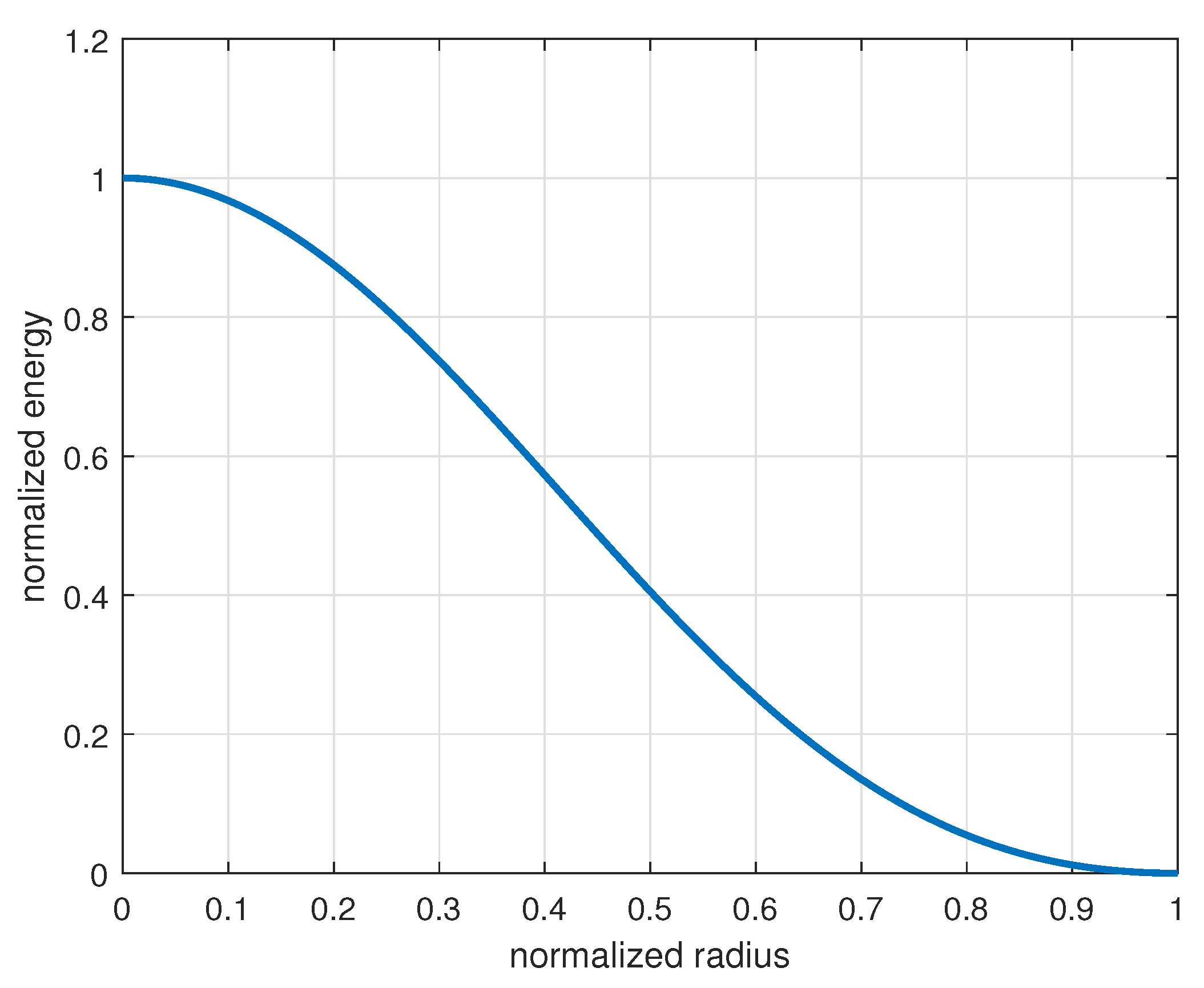
and the profile of the energy gap turns out to be modulated by $j_0^2\left(\pi \frac{r}{r_{CD}}\right)$ (see Figure 2).

Now, we make a number of further considerations beyond the exact calculation carried out thus far, allowing the density of the oscillating charges and its neutralizing background charge density to vary to a certain extent, while maintaining its uniformity inside the CD through migration within the material. We realize that the spatial modulation of the energy gap inside the CD produces a gradient that pulls the charges towards the center of the CD, thereby increasing the density to the maximum value compatible with the other terms of the energy per particle (which have been neglected in our previous calculation), namely, the electrostatic Coulomb repulsion among particles and Pauli repulsion in case of fermions. As a final result, the system reaches an equilibrium density at which the attractive coherent potential is counterbalanced by the repulsive short-range terms.

The density on the outside is lower than that inside the CD due to the equilibrium of the chemical potential, while a sharp variation of the density is present at the boundary of the CD, implying a difference between the plasma frequency inside and outside the CD. The mismatch of the dispersion relations inside and outside the CD implies the total reflection of the EM field at the interface. Thus, a natural resonating cavity is generated.

In particular, as the dispersion relation of the renormalized radiating field ${\omega }^{\prime }=\sqrt{|\overrightarrow{k}{|}^2+{\omega }_p^2}$ is different from Equation (45), the electromagnetic field cannot propagate through the vacuum and remains trapped inside the material. In other words, the described mechanism accounts for the formation of a self-generated natural QED cavity after the density of the charges overcomes a certain threshold.

Such configurations may well be identified as new emerging mesoscopic structures able to justify particular properties of matter that display intrinsic quantum features.

The spatial modulation of the fields implies that the average energy gap throughout the CD is provided by

$$<\delta E>=\delta E\left(0\right)\frac{4\pi {\int }_0^{r_{CD}}{r}^{2}dr{j}_0^2\left(\pi \frac{r}{r_{CD}}\right)}{\frac{4}{3}\pi r_{CD}^3}=\frac{3}{2{\pi }^2}\delta E\left(0\right)\simeq 0.152\delta E\left(0\right)$$

(52)

9. Discussion

Most extant theories of condensed matter do not consider the radiative component of the electromagnetic field to play a central role, due to its being strongly shielded by the high density of the charges and the conception that only those electrostatic forces generated by the constituents of matter are important. This is indeed true at most times, as the attenuation length for the electromagnetic field is typically much smaller than the wavelength of the radiating field. However, in certain circumstances the attenuation can be compensated by a positive optical gain of the material, as happens, for instance, in solid state lasers and optical microcavities in which exciton-polaritons are formed [29,30,31]. A similar mechanism is at play in the problem under study.

In the previous sections, we have shown how, via instability of the QED vacuum, when the temperature is low enough a spontaneous phase transition is possible for a system of charges oscillating around equilibrium positions and immersed in a spatially modulated neutralizing charge density of opposite sign.

In Section 8, we reported that the typical spatial dimension of the coherence domains is fixed by the wavelength $\lambda$ of the radiation field trapped inside the domains. However, this dimension is usually much smaller than the typical dimension of bulk material, meaning that we should expect the bulk material to contain a collection of coherence domains. Such domains are characterized by a single macroscopic wave function, an order parameter, and a well-determined quantum phase, which together confer intrinsically macroscopic quantum properties on the domains.

The arguments developed in the present work are valid for bosonic states of matter and remain valid for fermion systems when a trial state $|\mathrm{\Omega }\rangle$ incorporating the anti-symmetry of the global wave function has been defined. This theoretical development will be addressed in a future work.

Regarding the energetic stability of the solutions, and considering the fact that in [9] the spatial distribution of matter is two-dimensional, while in our case it is three-dimensional, a substantial difference between the results reached in [9] and ours lies in the fact that the states considered in [9] are plane waves, whereas in the present work we have considered coherent states with spatial size and oscillation that remain limited thanks to the intervention of nonlinear forces. This fact avoids a divergent energy gap associated with such coherent states.

The physical system analyzed in this work is at zero temperature. A next step will be to consider its thermal properties. While this topic will be addressed in a future work, we can anticipate that thermal excitations cause a portion of the particles forming the coherent state to populate the levels of the single quasi-particle spectrum. The net result is the formation of a two-fluid system similar to that proposed for superfluid helium [32]. Within this theoretical framework, all the properties associated with the degrees of freedom of the quasi-particles of the consolidated condensed matter theory involve the incoherent fraction, and only at low temperatures does the coherent fraction macroscopically manifest its intrinsically coherent characteristics.

A similar coherent condensation mechanism produced by the electromagnetic field can occur in atomic or molecular systems with an electric dipole. In this case, the electromagnetic field couples to two electronic levels displaying a sufficiently large electric dipole. A very interesting example is represented by liquid water [33,34].

In general, in a physical system made up of different types of charges with sufficiently high density, various types of electrodynamic coherence associated with different degrees of freedom of the charges can coexist. For instance, in a crystal the valence or conduction electrons and ions can form their own coherent states, each one resonating with the electromagnetic field at their specific plasmon polariton frequency.

10. Conclusions

In this work, we have defined and mathematically solved the problem of determining the lowest energy state of a large number of charged bosons coupled to selected modes of the electromagnetic field and harmonically oscillating around their equilibrium positions defined by the vertices of a crystal with lattice spacing much smaller than the wavelength of the modes of the electromagnetic field.

The equilibrium positions are determined by a periodic electrostatic potential, which we have called the jellium crystal, which implements global charge neutrality and localization.

The solution we have found corresponds to a state in which both the electromagnetic and matter fields are coherent and oscillate in quadrature and with a renormalized frequency with respect to the perturbative solution.

The energy content of this state is lower than that of the perturbative state. This is not in contrast with the no-go theorems mentioned in the introduction, as our calculation takes into account the contribution of the wave vectors in all directions. The aforementioned theorems consider only a single wave vector, and as such do not apply to our case.

The calculated energetic gap is not divergent, as it depends on the maximum oscillation that the charges can perform, which is limited by the finite size of the elementary cells of the crystal.

From a heuristic analysis of the solutions we found, we have defined a spatial region called the coherence domain (CD), the size of which is provided by the wavelength of the field and in which both the matter and electromagnetic fields are described by single macroscopic wave functions spatially modulated by the spherical harmonic $j_0\left(\right|\overrightarrow{k}\left|r\right)$, where r is the distance from the center of the domain and $|\overrightarrow{k}|$ is the modulus of the wave vectors of the e.m. field. Due to the modulation of the fields, the energy gap depends on r, resulting in an average gap $\langle \delta E\rangle$ over the coherence domain which is about 15% of the maximum gap $\delta E\left(0\right)$. We numerically evaluated this average value for a case involving protons loaded in the octahedral voids of a typical FCC crystal, resulting in a gap of $-1$ eV per particle.

The coherent electromagnetic field remains confined within the domain due to the mismatch of the dispersion relation on the edge of the domain, and as such cannot propagate, forming a natural QED cavity. If the crystal is spatially larger than the size of a single coherence domain, the material is filled with a collection of CDs.

It should be noted that the present analysis was performed at zero temperature; the thermodynamics of the coherence domains will be presented in a future work.

Although our calculation is in reference to bosons, it may apply to protons bound in a crystal matrix as well if their density is very low compared to the density of available states. Indeed, the overlap of the single particle wave functions of the protons located in different lattice cells is negligible, implying a negligible contribution to the exchange integrals, and the antisymmetrization of the global wave function of protons has practically no effect.