Article

Application of Aboodh Homotopy Perturbation Transform Method for Fractional-Order Convection–Reaction–Diffusion Equation within Caputo and Atangana–Baleanu Operators

Department of Basic Sciences, Preparatory Year Deanship, King Faisal University, Al-Ahsa 31982, Saudi Arabia
Symmetry 2023, 15(2), 453; https://doi.org/10.3390/sym15020453
Submission received: 28 December 2022 / Revised: 29 January 2023 / Accepted: 3 February 2023 / Published: 8 February 2023

Abstract

:
This article is an analysis of fractional nonlinear convection–reaction–diffusion equations involving the fractional Atangana–Baleanu and Caputo derivatives. An efficient Aboodh homotopy perturbation transform method, which combines the homotopy perturbation method with the Aboodh transformation, is applied to investigate this fractional-order proposed model, analytically. A modified technique known as the Aboodh homotopy perturbation transform method is formulated to approximate these derivatives. The analytical simulation is investigated graphically as well as in tabular form.

1. Introduction

In recent decades, rapid and very efficient algorithms for fractional differential equations have been developed. The reason for this rapid progress is that the fractional derivatives and equations effectively represent the majority of complicated phenomena, such as the mechanical properties of materials, memory-dependent phenomena, groundwater flow difficulties, anomalous diffusion and control theory. In addition, mathematical models based on fractional-order derivatives are more realistic and accurately reflect a wide range of natural phenomena [1,2,3]. The Riemann–Liouville fractional derivative and Caputo’s fractional derivative are the most often used fractional derivatives; however, they have certain restrictions because their definitions entail a solitary kernel, which can have an impact on physical difficulties [4,5,6]. Fractional-order problems refer to mathematical models that involve derivatives of a non-integer order. These types of models are commonly used to describe complex systems in various fields, such as physics, engineering, and biology.
One example of a physical problem that can be modeled using fractional-order equations is the fractional Burgers equation. This equation is a generalization of the classical Burgers equation, which describes the dynamics of fluid flow in a channel. The fractional Burgers equation includes a fractional derivative term, which accounts for the effects of viscoelasticity and memory on the fluid flow. This equation has been used to model a variety of physical systems, including blood flow in vessels, heat conduction in solids, and the dynamics of turbulence [7,8].
Another example of a physical problem that can be modeled using fractional-order equations is the fractional Schrodinger equation. This equation is a generalization of the classical Schrodinger equation, which describes the dynamics of quantum systems. The fractional Schrodinger equation includes a fractional derivative term, which accounts for the effects of quantum memory on the system. This equation has been used to model a variety of physical systems, including quantum tunneling, quantum dynamics in disordered systems, and the dynamics of quantum entanglement [9,10].
Additionally, it would be beneficial to discuss the advantages and limitations of using fractional-order models compared to traditional integer-order models in solving real-world problems. Examples of real-world applications where fractional-order models have been successfully applied, such as in the fields of fluid dynamics, control systems, and signal processing, should also be included. This will not only make the paper more interesting but also demonstrate the practical relevance of the proposed methods.
A novel definition of the fractional operator with a non-singular kernel based on the exponential function was put out by Caputo and Fabrizio [11] in 2015. This definition has the power to describe heterogeneities and structures of many sizes that fractional systems with a single kernel are unable to represent adequately. Numerous researchers have looked into different fractional mathematical models, such as the groundwater flow [12], El Nino-Southern oscillation model [13], the fractional epidemiological model for computer viruses [14], groundwater pollution equation [15] and evolution equations [16] using the Caputo–Fabrizio (CF) operator concept.
Recently, Atangana and Baleanu [17] suggested a new derivative based on the extended Mittag–Leffler term to overcome the fractional model derivatives [18,19] with the nonlocal and non-singular kernels. The possibility that there are nonlocal schemes that effectively define the material heterogeneities and variations of various scales, which cannot be adequately described by traditional local theory or by a local fractional model with a singular kernel, gave rise to interest in this novel operator with a non-singular kernel. Researchers have utilized the AB derivative in various ways to mimic real-world circumstances, such as Gomez Aguilar et al. [20], who proposed an alternative solution for an electromagnetic wave in dielectric media by using the fractional AB derivative. Alkahtani examined the dynamic of Chua’s problem using a newly created AB operator and discovered unexpected chaotic phenomena [21]. Owolabi [22] examined the simulation and modeling of an ecological framework using the Adams–Bashforth technique with two steps and the AB derivative. A helpful tool for representing nonlinear events in scientific and engineering models is the fractional differential equation. In applied mathematics and engineering, partial differential equations, particularly nonlinear ones, have been utilized to simulate a wide range of scientific phenomena. Fractional-order partial differential equations (FPDEs) allowed researchers to recognize and model a wide range of significant and real-world physical issues in parallel with their work in the physical sciences. It has always been claimed how important it is to obtain approximations for them using either numerical or analytical methods. As a result, symmetry analysis is an excellent tool for understanding partial differential equations, particularly when looking at equations derived from accounting-related mathematical ideas. Most natural observations lack symmetry, even though symmetry is the cornerstone to nature. Unexpected symmetry-breaking occurrences is a sophisticated method of hiding symmetry. Finite and infinitesimal symmetry are the two types. Finite symmetries can either be discrete or continuous. Parity and temporal inversion are discrete natural symmetries, whereas space is a continuous transformation. Patterns have always captivated mathematicians. In the seventeenth century, the classification of spatial and planar patterns began. Regrettably, a precise solution of fractional nonlinear differential equations has shown to be exceedingly challenging [23,24].
Real implementations of physics, applied biology, science, and technology are only a handful of the seemingly unconnected situations in which nonlinear occurrences can arise. The most common type of nonlinear problem is partial differential equations (PDEs). We refer to modeled nonlinear reaction–diffusion situations as a class of PDEs. In several physical (real-world) situations, such as the dynamics of biological systems, groundwater processes, image analysis, machine learning, fractals, and mechatronics, phase transition in electrical electronic and nonlinear diffusion model is considered to be an important class of parabolic equations [25,26,27].
In this article, the Aboodh transformation, combined with the Caputo and Atangana–Baleanu derivatives, is used to analyze three special convection–reaction–diffusion equations (CRDEs). Consider the following fractional CRDE:
D ϑ Θ ( ξ , ϑ ) = Θ ξ ξ ( ξ , ϑ ) + Θ ( ξ , ϑ ) + Θ ( ξ , ϑ ) Θ ξ ( ξ , ϑ ) Θ 2 ( ξ , ϑ ) ,
with the initial condition
Θ ( ξ , 0 ) = 1 + e ξ ,
and
D ϑ Θ ( ξ , ϑ ) = Θ ξ ξ ( ξ , ϑ ) Θ ξ ( ξ , ϑ ) + Θ ( ξ , ϑ ) + Θ ( ξ , ϑ ) Θ ξ ( ξ , ϑ ) Θ 2 ( ξ , ϑ ) ,
with the initial condition
Θ ( ξ , 0 ) = e ξ ,
and
D ϑ Θ ( ξ , ϑ ) = Θ ξ ξ ( ξ , ϑ ) ( 1 + 4 ξ 2 ) Θ ( ξ , ϑ ) ,
with the initial condition
Θ ( ξ , 0 ) = e ξ 2 .
Convection, reaction and diffusion are implied by the convection–reaction–diffusion equation. Convection refers to the flow of molecules from one region (fluid) to another. In contrast, diffusion refers to the random movement of particles from a high-concentration zone to a low-concentration region. Lastly, reaction refers to the decomposition, adsorption, and chemical reactions of a substance with other components and the biodegradation of pollutants. The convection–reaction–diffusion equation (CRD) appears in the mathematical modeling of numerous essential domains of applied research, including mechanics, kinematics, ecology, and hydrological. For example, the given problems have been used to describe the following: theory of combustion and detonation, transport phenomena in porous media, chemical reaction–diffusion, population dynamics and mathematical biology, finance, heat transfer in a draining film [16], fluid flow as well as transport chemistry in the atmosphere. In hydrology, this form of equation models the transport of microbe nutrients and adsorbing contaminants schemes in groundwater [28,29,30].
In numerous applications, the solutions of the nonlinear convection–reaction–diffusion equation are crucial. Numerous researchers employ numerical approaches to approximate the solution of these equations due to the challenges in obtaining analytical solutions. Numerous studies have been conducted on numerical solutions for nonlinear (CRD) problems. The finite difference method is one of the simplest and oldest techniques for solving (CRD) equations. For the solution of partial differential equations, essentially non-oscillatory (ENO) and weighted ENO (WENO) methods have been devised in [31,32]. In [33], the application and comparison of these approaches are described to solve convection diffusion. Standard finite difference creates numerical instabilities, such as oscillations and numerical dispersion, in the solution approximations for specific problems. Ref. [34] uses a nonstandard finite difference method to overcome numerical instability. In the meantime, a novel Eulerian–Lagrangian numerical approach was published [35] that integrated the precise time stepping scheme with the finite difference method. In ref. [36], a new finite difference method based on a particular grid was presented; the approach includes discretization in time utilizing Crank–Nicolson and backward Euler finite difference schemes. For the spatial discretization, one can employ the method described in ref. [37] which proposes the streamline-upwind Petrov–Galerkin (SUPG) approach. The SUPG-SC (streamline-upwind Petrov–Galerkin and shock capturing) technique can minimize the physical oscillation in the cross-wind direction, according to new research [38,39]. In [40], various problems dominated by nonlinear convection are handled using the discontinuous Galerkin approach and the shock-capturing methodology. In [41], the adaptive discontinuous Galerkin technique is expanded.

2. Basic Definitions

In this section, a few definitions, theorems and property that will be useful in this article are given.
Definition 1.
The Aboodh transformation (AT) of a term Θ ( ϑ ) with exponential-order
C = Θ : | Θ ( ϑ ) | < B e p j | ϑ | , if ϑ ( 1 ) i × [ 0 , ) , j = 1 , 2 ; B , p 1 , p 2 > 0
is written as
A [ Θ ( ϑ ) ] = M ( ψ ) ,
and expressed as
A [ Θ ( ϑ ) ] = 1 ψ 0 Θ ( ϑ ) e ψ ϑ d ϑ = M ( ψ ) , p 1 ψ p 2 .
Obviously, the AT is linear as the Laplace transformation (LT).
Definition 2.
The Mittag–Leffler function is a special function that often occurs naturally in the result of fractional-order calculus, and it is given as follows:
E ( Z ) = ρ = 0 Z ρ Γ ( ρ + 1 ) , , Z C , R e ( ) 0 ,
In generalized type, it is given as follows:
E , γ ξ = ρ = 0 Z ρ ( ξ ) ρ Γ ( γ + ρ ) ρ ! , , γ , Z C , Re ( ) 0 , Re ( γ ) 0 ,
Furthermore, we suppose ( ξ ) ρ to be the Pochhammer’s symbols.
Definition 3.
Let Θ H 1 ( 0 , 1 ) and 0 < < 1 , then the fractional AB derivative is defined as
0 A B C D ϑ Θ ( ϑ ) = N ( ) 1 0 ϑ Θ ( x ) E ( ϑ x ) 1 d x .
Definition 4.
Let Θ H 1 ( 0 , 1 ) and 0 < < 1 , then the fractional AB derivative is expressed in the sense of Riemann–Liouville:
0 A B R D ϑ Θ ( ϑ ) = N ( ) 1 d d ϑ 0 ϑ Θ ( x ) E ( ϑ x ) 1 d x ,
The normalization term N ( ) > 0 satisfies the conditions N ( 0 ) = N ( 1 ) = 1 .
Theorem 1.
The LT of AB fractional operator according to the sense of Caputo is as follows:
L 0 A B C D ϑ Θ ( ϑ ) = N ( ) 1 × s Θ ( s ) s 1 Θ ( 0 ) s + 1 ,
Furthermore, the LT of AB fractional operator according to the Riemann–Liouville is defined as
L 0 A B R D ϑ Θ ( ϑ ) = N ( ) 1 × s Θ ( s ) s + 1 .
Theorem 2.
Let , γ C , with R e ( ) > 0 , R e ( γ ) > 0 , the AT of ϑ γ 1 E , ξ ξ Ω ϑ is expressed as
ϑ γ 1 E , ξ ξ Ω ϑ = 1 ψ γ + 1 1 Ω ψ ξ , Ω ψ < 1 .
Theorem 3.
If M ( ψ ) is the AT of Θ ( ϑ ) C and Θ ( ψ ) is the LT of Θ ( ϑ ) C , then the AT of fractional AB derivative according to the sense of Caputo is expressed as
M 0 A B C D ϑ Θ ( ϑ ) = N ( ) M ( ψ ) ψ 2 Θ ( 0 ) 1 + ψ .
Theorem 4.
Suppose that M ( ψ ) is the AT of Θ ( ϑ ) C and Θ ( ψ ) is the LT of Θ ( ϑ ) C , then the AT of fractional AB derivative according to the sense Riemann–Liouville is expressed as
M 0 A B R D ϑ Θ ( ϑ ) = N ( ) M ( ψ ) 1 + ψ .

3. General Implementations of the AHPTM

Consider the general fractional partial differential equations
D ϑ Θ ( ξ , ϑ ) + L ( Θ ( ξ , ϑ ) ) + N ( Θ ( ξ , ϑ ) ) = θ ( ξ , ϑ ) , ( ξ , ϑ ) [ 0 , 1 ] × [ 0 , T ] , κ 1 < < κ ,
with the initial condition
z Θ ϑ z ( ξ , 0 ) = z ( ξ ) , z = 0 , 1 , , κ 1 .
In Equation (7), L is linear and N nonlinear terms. The Caputo fractional derivative can be written as
Θ ( ξ , ϑ ) = 1 ϖ ( Θ ( ξ , ϑ ) A [ L ( Θ ( ξ , ϑ ) ) + N ( Θ ( ξ , ϑ ) ) ] ) + 1 ϖ 2 Θ ( ξ , 0 ) .
The fractional AB derivative is given as
Θ ( ξ , ϑ ) = 1 + ϖ N ( ) ( Θ ( ξ , ϑ ) A [ L ( Θ ( ξ , ϑ ) ) + N ( Θ ( ξ , ϑ ) ) ] ) + 1 ϖ 2 Θ ( ξ , 0 ) .
where the homotopy parameter ρ is defined as
Θ ( ξ , ϑ ) = j = 0 ρ j Θ j ( ξ , ϑ ) , j = 0 , 1 , 2 ,
The non-linear components in Equation (7) can be written as
N [ Θ ( ξ , ϑ ) ] = j = 0 ρ j Θ j ( ξ , ϑ ) ,
and the nonlinear terms Θ j ( ξ , ϑ ) are defined as
Θ j ( Θ 0 , Θ 1 , , Θ j ) = 1 j ! j ν j N j = 0 ν j Θ j ν = 0 , j = 0 , 1 , 2 ,
We achieved the component of the Caputo operator result by putting Equations (11) and (12) into Equation (9):
j = 0 ρ j Θ ( ξ , ϑ ) = ρ 1 ϖ A L j = 0 ρ j Θ j ( ξ , ϑ ) + j = 0 ρ j Θ j ( ξ , ϑ ) + 1 ϖ ( Θ ( ξ , ϑ ) ) + 1 ϖ 2 Θ ( ξ , 0 ) .
The recursive connection that is the solution of the AB derivative, by putting Equations (11) and (12) into Equation (10), is given by
j = 0 ρ j Θ ( ξ , ϑ ) = ρ 1 + ϖ N ( ) A L j = 0 ρ j Θ j ( ξ , ϑ ) + j = 0 ρ j Θ j ( ξ , ϑ ) + 1 + ϖ N ( ) ( Θ ( ξ , ϑ ) ) + 1 ϖ 2 Θ ( ξ , 0 ) .
Thus, Equations (14) and (15), when solved with respect to ρ , are defined as
ρ 0 : Θ 0 ( ξ , ϑ ) = 1 ϖ ( Θ ( ξ , ϑ ) ) + 1 ϖ 2 Θ ( ξ , 0 ) , ρ 1 : Θ 1 ( ξ , ϑ ) = 1 ϖ A L ( Θ 0 ( ξ , ϑ ) ) + Θ 0 ( ξ , ϑ ) , ρ 2 : Θ 2 ( ξ , ϑ ) = 1 ϖ A L ( Θ 1 ( ξ , ϑ ) ) + Θ 1 ( ξ , ϑ ) , ρ j + 1 : Θ j + 1 ( ξ , ϑ ) = 1 ϖ A L ( Θ j ( ξ , ϑ ) ) + Θ j ( ξ , ϑ ) .
Moreover, the AB homotopy is calculated as
ρ 0 : Θ 0 ( ξ , ϑ ) = 1 + ϖ N ( ) Θ ( ξ , ϑ ) + 1 ϖ 2 Θ ( ξ , 0 ) , ρ 1 : Θ 1 ( ξ , ϑ ) = 1 + ϖ N ( ) A L ( Θ 0 ( ξ , ϑ ) ) + Θ 0 ( ξ , ϑ ) , ρ 2 : Θ 2 ( ξ , ϑ ) = 1 + ϖ N ( ) A L ( Θ 1 ( ξ , ϑ ) ) + Θ 1 ( ξ , ϑ ) , ρ j + 1 : Θ j + 1 ( ξ , ϑ ) = 1 + ϖ N ( ) A L ( Θ j ( ξ , ϑ ) ) + Θ j ( ξ , ϑ ) .
When ρ 1 is applied, suppose that Equations (16) and (17) are the approximated solution to Equations (14) and (15), and the result is
Θ j ( ξ , ϑ ) = j = 0 j Θ j ( ξ , ϑ ) .
Applying the inverse AT to Equation (18) and calculating the result of Equation (7) gives
Θ ( ξ , ϑ ) Θ j ( ξ , ϑ ) = A 1 | { Θ j ( ξ , ϑ ) } .

4. Numerical Examples

Example 1.
In this section, apply the AT of Equations (1)–(6). First, solve Equation (1) with the help of the Caputo operator [42]:
Θ ( ξ , ϑ ) = 1 ϖ A Θ ξ ξ ( ξ , ϑ ) + Θ ( ξ , ϑ ) + Θ ( ξ , ϑ ) Θ ξ ( ξ , ϑ ) Θ 2 ( ξ , ϑ ) + 1 ϖ 2 Θ ( ξ , 0 ) .
To investigate Equation (20), we apply the AHPTM
j = 0 ρ j Θ j ( ξ , ϑ ) = ρ 1 ϖ A j = 0 ρ j Θ j ( ξ , ϑ ) ξ ξ + j = 0 ρ j Θ j ( ξ , ϑ ) + ρ 1 ϖ A j = 0 ρ j Θ j ( ξ , ϑ ) + 1 ϖ 2 Θ ( ξ , 0 ) .
By applying the inverse AT to Equation (21), we obtain
j = 0 ρ j Θ j ( ξ , ϑ ) = ρ A 1 1 ϖ A j = 0 ρ j Θ j ( ξ , ϑ ) ξ ξ + j = 0 ρ j Θ j ( ξ , ϑ ) + ρ A 1 1 ϖ A j = 0 ρ j Θ j ( ξ , ϑ ) + A 1 [ 1 ϖ 2 Θ ( ξ , 0 ) ] .
In Equation (22), the Θ j ( . ) represents the non-linear functions in Equation (14):
Θ 0 ( Θ ) = Θ 0 ( Θ 0 ) ξ ( Θ 0 ) 2 , Θ 1 ( Θ ) = Θ 0 ( Θ 1 ) ξ + Θ 1 ( Θ 0 ) ξ 2 Θ 0 Θ 1 , Θ 2 ( Θ ) = Θ 0 ( Θ 2 ) ξ + Θ 1 ( Θ 1 ) ξ + Θ 2 ( Θ 0 ) ξ 2 Θ 0 Θ 2 ( Θ 2 ) 2 ,
The function of the Caputo derivative result is achieved by calculating the powers of ρ:
ρ 0 : Θ 0 ( ξ , ϑ ) = A 1 [ 1 ϖ 2 1 + e ( ξ ) ] = 1 + e ( ξ ) , ρ 1 : Θ 1 ( ξ , ϑ ) = A 1 [ 1 ϖ A [ L ( Θ 0 ( ξ , ϑ ) ) ] ] + A 1 [ 1 ϖ A [ Θ 0 ( ξ , ϑ ) ] ] = 1 + e ( ξ ) ϑ Γ ( + 1 ) , ρ 2 : Θ 2 ( ξ , ϑ ) = A 1 [ 1 ϖ A [ L ( Θ 1 ( ξ , ϑ ) ) ] ] + A 1 [ 1 ϖ A [ Θ 1 ( ξ , ϑ ) ] ] = 1 + e ( ξ ) ϑ 2 Γ ( 2 + 1 ) ,
Thus, we obtain
Θ ( ξ , ϑ ) = 1 + e ( ξ ) + 1 + e ( ξ ) ϑ Γ ( + 1 ) + 1 + e ( ξ ) ϑ 2 Γ ( 2 + 1 ) + ,
Θ ( ξ , ϑ ) = 1 + e ( ξ ) 1 + ϑ Γ ( + 1 ) + ϑ 2 Γ ( 2 + 1 ) + .
The exact result is Θ ( ξ , ϑ ) = 1 + e ( ξ + ϑ ) .
Now, we apply the AB operator in Equation (1) to obtain
Θ ( ξ , ϑ ) = 1 + ϖ N ( ) A Θ ξ ξ ( ξ , ϑ ) + Θ ( ξ , ϑ ) + Θ ( ξ , ϑ ) Θ ξ ( ξ , ϑ ) Θ 2 ( ξ , ϑ ) + 1 ϖ 2 Θ ( ξ , 0 ) .
Applying AHPTM to Equation (26), one can obtain
j = 0 ρ j Θ j ( ξ , ϑ ) = ρ 1 + ϖ N ( ) A j = 0 ρ j Θ j ( ξ , ϑ ) ξ ξ + j = 0 ρ j Θ j ( ξ , ϑ ) + ρ 1 + ϖ N ( ) A j = 0 ρ j Θ j ( ξ , ϑ ) + 1 ϖ 2 Θ ( ξ , 0 ) .
By applying the inverse AT to Equation (27), we have
j = 0 ρ j Θ j ( ξ , ϑ ) = ρ A 1 1 + ϖ N ( ) A j = 0 ρ j Θ j ( ξ , ϑ ) ξ ξ j = 0 ρ j Θ j ( ξ , ϑ ) + ρ A 1 1 + ϖ N ( ) A j = 0 ρ j Θ j ( ξ , ϑ ) + A 1 [ 1 ϖ 2 Θ ( ξ , 0 ) ] .
Equation (28) contains Θ j ( . ) functions, which are non-linear polynomials specified in Equation (13):
ρ 0 : Θ 0 ( ξ , ϑ ) = A 1 [ 1 ϖ 2 1 + e ( ξ ) ] = 1 + e ( ξ ) , ρ 1 : Θ 1 ( ξ , ϑ ) = A 1 [ 1 + ϖ N ( ) A [ L ( Θ 0 ( ξ , ϑ ) ) ] ] + A 1 [ 1 + ϖ N ( ) A [ Θ 0 ( ξ , ϑ ) ] ] = 1 + e ξ N ( ) ϑ Γ ( + 1 ) + 1 , ρ 2 : Θ 2 ( ξ , ϑ ) = A 1 [ 1 + ϖ N ( ) A [ L ( Θ 1 ( ξ , ϑ ) ) ] ] + A 1 [ 1 + ϖ N ( ) A [ Θ 1 ( ξ , ϑ ) ] ] = 1 + e ξ N 2 ( ) ( ϑ ) 2 Γ ( 2 + 1 ) + 2 ( 1 ) ϑ Γ ( + 1 ) + ( 1 ) 2 ,
with the help of AB derivative, one can obtain
Θ ( ξ , ϑ ) = = 0 n Θ ( ξ , ϑ ) = 1 + e ξ + 1 + e ξ N ( ) ϑ Γ ( ) + 1 + 1 + e ξ N 2 ( ) 2 ϑ 2 Γ ( 2 + 1 ) + ( 1 ) ϑ 2 Γ ( + 1 ) + ( 1 ) 2 + ,
The exact result is Θ ( ξ , ϑ ) = 1 + e ( ξ + ϑ ) .
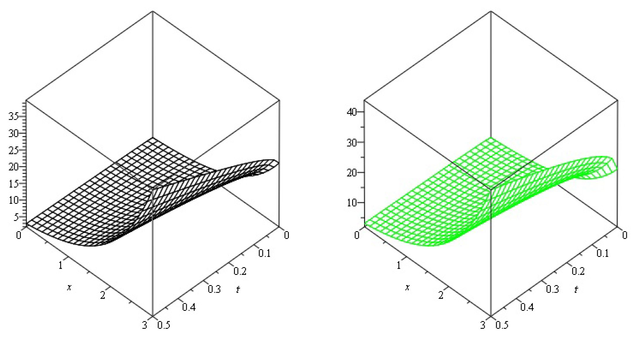
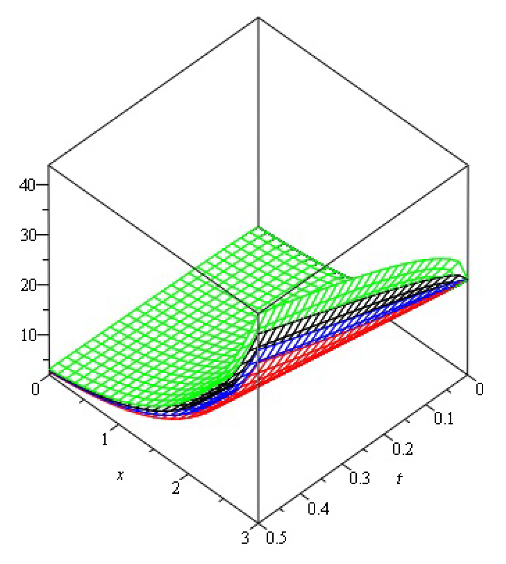
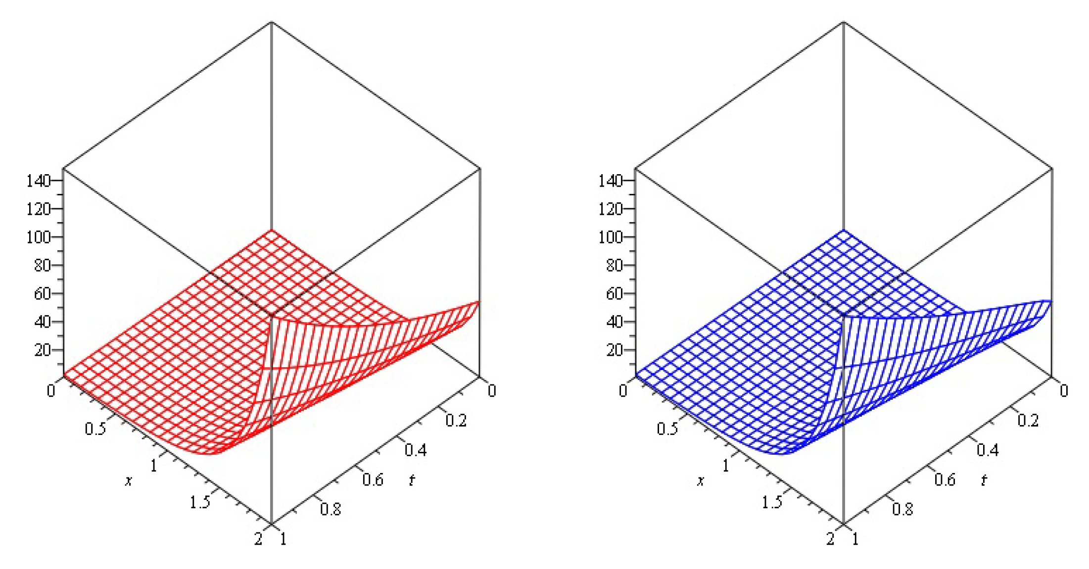
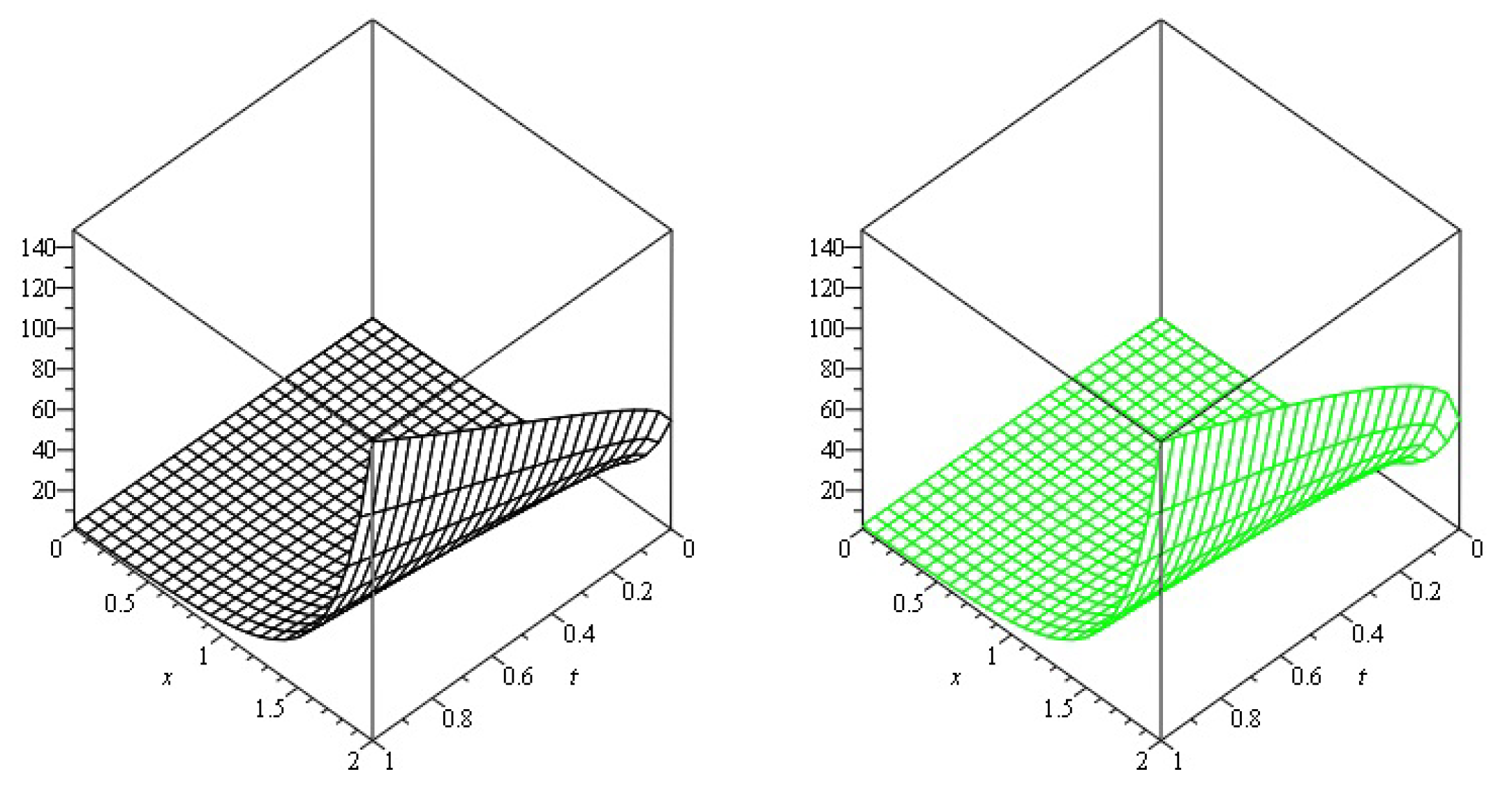
In Figure 1, the analytical solution of fractional order of = 1 and 0.8 Example 1. Figure 2, the analytical solution of fractional order of = 0.6 and 0.4 Example 1. Figure 3, the various fractional-order solution of ℘ Example 1. In Table 1, the different fractional order of ℘ comparison of Example 1.
Example 2.
Apply the AT of Equations (3) and (4). First solve Equation (3) with the help of the Caputo operator [42]:
Θ ( ξ , ϑ ) = 1 ϖ A Θ ξ ξ ( ξ , ϑ ) Θ ξ ( ξ , ϑ ) + Θ ( ξ , ϑ ) + Θ ( ξ , ϑ ) Θ ξ ( ξ , ϑ ) Θ 2 ( ξ , ϑ ) + 1 ϖ 2 Θ ( ξ , 0 ) .
To investigate Equation (31), we apply the AHPTM
j = 0 ρ j Θ j ( ξ , ϑ ) = ρ 1 ϖ A j = 0 ρ j Θ j ( ξ , ϑ ) ξ ξ + j = 0 ρ j Θ j ( ξ , ϑ ) j = 0 ρ j Θ j ( ξ , ϑ ) ξ + ρ 1 ϖ A j = 0 ρ j Θ j ( ξ , ϑ ) + 1 ϖ 2 Θ ( ξ , 0 ) .
By applying the inverse AT to Equation (32), we obtain
j = 0 ρ j Θ j ( ξ , ϑ ) = ρ A 1 1 ϖ A j = 0 ρ j Θ j ( ξ , ϑ ) ξ ξ + j = 0 ρ j Θ j ( ξ , ϑ ) j = 0 ρ j Θ j ( ξ , ϑ ) ξ + ρ A 1 1 ϖ A j = 0 ρ j Θ j ( ξ , ϑ ) + A 1 [ 1 ϖ 2 Θ ( ξ , 0 ) ] .
In Equation (22), the Θ j ( . ) represents the non-linear functions in Equation (14):
Θ 0 ( Θ ) = Θ 0 ( Θ 0 ) ξ ( Θ 0 ) 2 , Θ 1 ( Θ ) = Θ 0 ( Θ 1 ) ξ + Θ 1 ( Θ 0 ) ξ 2 Θ 0 Θ 1 , Θ 2 ( Θ ) = Θ 0 ( Θ 2 ) ξ + Θ 1 ( Θ 1 ) ξ + Θ 2 ( Θ 0 ) ξ 2 Θ 0 Θ 2 ( Θ 2 ) 2 ,
The functions of the Caputo derivative result are achieved by calculating the powers of ρ:
ρ 0 : Θ 0 ( ξ , ϑ ) = A 1 [ 1 ϖ 2 1 + e ( ξ ) ] = e ( ξ ) , ρ 1 : Θ 1 ( ξ , ϑ ) = A 1 [ 1 ϖ A [ L ( Θ 0 ( ξ , ϑ ) ) ] ] + A 1 [ 1 ϖ A [ Θ 0 ( ξ , ϑ ) ] ] = e ( ξ ) ϑ Γ ( + 1 ) , ρ 2 : Θ 2 ( ξ , ϑ ) = A 1 [ 1 ϖ A [ L ( Θ 1 ( ξ , ϑ ) ) ] ] + A 1 [ 1 ϖ A [ Θ 1 ( ξ , ϑ ) ] ] = e ( ξ ) ϑ 2 Γ ( 2 + 1 ) ,
Thus, we obtain
Θ ( ξ , ϑ ) = e ( ξ ) + e ( ξ ) ϑ Γ ( + 1 ) + e ( ξ ) ϑ 2 Γ ( 2 + 1 ) + ,
Θ ( ξ , ϑ ) = e ( ξ ) 1 + ϑ Γ ( + 1 ) + ϑ 2 Γ ( 2 + 1 ) + ,
The exact result is Θ ( ξ , ϑ ) = e ( ξ + ϑ ) .
Now, we apply the AB operator in Equation (3), and we obtain
Θ ( ξ , ϑ ) = 1 + ϖ N ( ) A Θ ξ ξ ( ξ , ϑ ) Θ ξ ( ξ , ϑ ) + Θ ( ξ , ϑ ) + Θ ( ξ , ϑ ) Θ ξ ( ξ , ϑ ) Θ 2 ( ξ , ϑ ) + 1 ϖ 2 Θ ( ξ , 0 ) .
Applying AHPTM to Equation (37), we achieve
j = 0 ρ j Θ j ( ξ , ϑ ) = ρ 1 + ϖ N ( ) A j = 0 ρ j Θ j ( ξ , ϑ ) ξ ξ + j = 0 ρ j Θ j ( ξ , ϑ ) j = 0 ρ j Θ j ( ξ , ϑ ) ξ + ρ 1 + ϖ N ( ) A j = 0 ρ j Θ j ( ξ , ϑ ) + 1 ϖ 2 Θ ( ξ , 0 ) .
By applying the inverse AT to above equation, we have
j = 0 ρ j Θ j ( ξ , ϑ ) = ρ A 1 1 + ϖ N ( ) A j = 0 ρ j Θ j ( ξ , ϑ ) ξ ξ + j = 0 ρ j Θ j ( ξ , ϑ ) j = 0 ρ j Θ j ( ξ , ϑ ) ξ + ρ A 1 1 + ϖ N ( ) A j = 0 ρ j Θ j ( ξ , ϑ ) + A 1 [ 1 ϖ 2 Θ ( ξ , 0 ) ] .
A comparison of both sides gives
ρ 0 : Θ 0 ( ξ , ϑ ) = A 1 [ 1 ϖ 2 e ξ ] = e ξ , ρ 1 : Θ 1 ( ξ , ϑ ) = A 1 [ 1 + ϖ N ( ) A [ L ( Θ 0 ( ξ , ϑ ) ) ] ] + A 1 [ 1 + ϖ N ( ) A [ Θ 0 ( ξ , ϑ ) ] ] = = e ξ N ( ) ϑ Γ ( ) + 1 , ρ 2 : Θ 2 ( ξ , ϑ ) = A 1 [ 1 + ϖ N ( ) A [ L ( Θ 1 ( ξ , ϑ ) ) ] ] + A 1 [ 1 + ϖ N ( ) A [ Θ 1 ( ξ , ϑ ) ] ] = = e ξ N 2 ( ) 2 ϑ 2 Γ ( 2 + 1 ) + ( 1 ) ϑ 2 Γ ( + 1 ) + ( 1 ) 2
With the help of the AB derivative, one can obtain
Θ ( ξ , ϑ ) = e ξ + e ξ N ( ) ϑ Γ ( ) + 1 + e ξ N 2 ( ) 2 ϑ 2 Γ ( 2 + 1 ) + ( 1 ) ϑ 2 Γ ( + 1 ) + ( 1 ) 2 + ,
The exact solution is Θ ( ξ , ϑ ) = e ( ϑ + ξ ) .
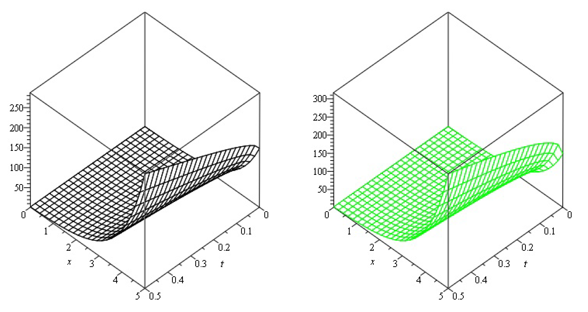
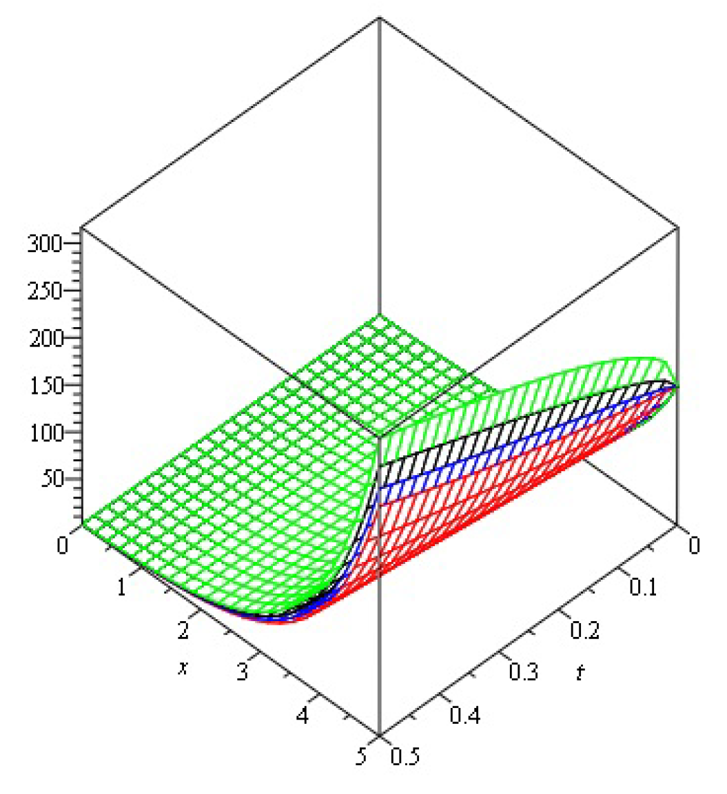
In Figure 4, the analytical solution of fractional order of = 1 and 0.8 Example 2. Figure 5, the analytical solution of fractional order of = 0.6 and 0.4 Example 2. Figure 6, the various fractional-order solution of ℘ Example 2. In Table 2, Example 2 error comparison at various fractional orders of ℘.
Example 3.
Finally, apply the AT of Equations (5) and (6). First solve Equation (5) with the help of the Caputo operator [42]:
Θ ( ξ , ϑ ) = 1 ϖ A Θ ξ ξ ( ξ , ϑ ) ( 1 + 4 ξ 2 ) Θ ( ξ , ϑ ) + 1 ϖ 2 Θ ( ξ , 0 ) .
To investigate Equation (42), we apply the AHPTM
j = 0 ρ j Θ j ( ξ , ϑ ) = ρ 1 ϖ A j = 0 ρ j Θ j ( ξ , ϑ ) ξ ξ ( 1 + 4 ξ 2 ) j = 0 ρ j Θ j ( ξ , ϑ ) + 1 ϖ 2 Θ ( ξ , 0 ) .
By applying the inverse AT to Equation (43), we obtain
j = 0 ρ j Θ j ( ξ , ϑ ) = ρ A 1 1 ϖ A j = 0 ρ j Θ j ( ξ , ϑ ) ( 1 + 4 ξ 2 ) j = 0 ρ j Θ j ( ξ , ϑ ) + A 1 1 ϖ 2 Θ ( ξ , 0 ) .
The functions of the Caputo derivative result are achieved by calculating the powers of ρ:
ρ 0 : Θ 0 ( ξ , ϑ ) = A 1 [ 1 ϖ 2 e ξ 2 ] = e ξ 2 , ρ 1 : Θ 1 ( ξ , ϑ ) = A 1 [ 1 ϖ A [ L ( Θ 0 ( ξ , ϑ ) ) ] ] , = e ξ 2 ϑ Γ ( + 1 ) , ρ 2 : Θ 1 ( ξ , ϑ ) = A 1 [ 1 ϖ A [ L ( Θ 1 ( ξ , ϑ ) ) ] ] , = e ξ 2 ϑ 2 Γ ( 2 + 1 ) ,
Thus, we obtain
Θ ( ξ , ϑ ) = e ξ 2 + e ξ 2 ϑ Γ ( + 1 ) + e ξ 2 ϑ 2 Γ ( 2 + 1 ) +
The exact solution is Θ ( ξ , ϑ ) = e ξ 2 + ϑ .
Now we apply the AB operator in Equation (5) to obtain
Θ ( ξ , ϑ ) = 1 + ϖ N ( ) A Θ ξ ξ ( ξ , ϑ ) ( 1 + 4 ξ 2 ) Θ ( ξ , ϑ ) + 1 ϖ 2 Θ ( ξ , 0 ) .
Applying AHPTM to Equation (47), we achieve
j = 0 ρ j Θ j ( ξ , ϑ ) = 1 + ϖ N ( ) A j = 0 ρ j Θ j ( ξ , ϑ ) ξ ξ ( 1 + 4 ξ 2 ) j = 0 ρ j Θ j ( ξ , ϑ ) + 1 ϖ 2 Θ ( ξ , 0 ) .
By applying the inverse AT to the above equation, we have
j = 0 ρ j Θ j ( ξ , ϑ ) = ρ A 1 1 + ϖ N ( ) A j = 0 ρ j Θ j ( ξ , ϑ ) ( 1 + 4 ξ 2 ) j = 0 ρ j Θ j ( ξ , ϑ ) + A 1 [ 1 ϖ 2 Θ ( ξ , 0 ) ] .
Comparison of both sides gives
ρ 0 : Θ 0 ( ξ , ϑ ) = A 1 [ 1 ϖ 2 sin ξ ] = e ξ 2 , ρ 1 : Θ 1 ( ξ , ϑ ) = A 1 1 + ϖ N ( ) A L ( Θ 0 ( ξ , ϑ ) ) = e ξ 2 N ( ) ϑ Γ ( ) + 1 , ρ 2 : Θ 2 ( ξ , ϑ ) = A 1 1 + ϖ N ( ) A L ( Θ 1 ( ξ , ϑ ) ) = e ξ 2 N 2 ( ) 2 ϑ 2 Γ ( 2 + 1 ) + ( 1 ) ϑ 2 Γ ( + 1 ) + ( 1 ) 2
With the help of AB derivative, one can obtain
Θ ( ξ , ϑ ) = e ξ 2 + e ξ 2 N ( ) ϑ Γ ( ) + 1 + e ξ 2 N 2 ( ) 2 ϑ 2 Γ ( 2 + 1 ) + ( 1 ) ϑ 2 Γ ( + 1 ) + ( 1 ) 2 + ,
The exact result is Θ ( ξ , ϑ ) = e ξ 2 + ϑ .
In Figure 7, the analytical solution of fractional order of = 1 and 0.8 Example 3. Figure 8, the analytical solution of fractional order of = 0.6 and 0.4 Example 3. Figure 9, the various fractional-order solution of ℘ Example 3. In Table 3, Example 3 error comparison at various fractional orders of ℘.

5. Conclusions

The main goal of this research is to develop an effective approach for solving fractional nonlinear convection–diffusion equations. The approximated solution of a specific fractional convection–reaction–diffusion (CRD) problem is determined in this study by employing a new integral transform technique called the Aboodh transformation. The given problems are first simplified utilizing Aboodh transformation, and then results are obtained by applying the perturbation method. The suggested method employs two fractional derivatives, the CD and AB operators. The solutions to fractional-order problems are explored and are found to be the optimal representation of the problems’ true dynamics. To demonstrate the validity of the proposed procedure, the findings are plotted and tabulated. The primary advantage of the proposed method is the rapid convergence of the series form solution to the precise solution. It is determined that the presented method for solving fractional partial differential equations is both easy and effective, and can thus be applied to other scientific problems.

Funding

This work was supported by the Deanship of Scientific Research, the Vice Presidency for Graduate Studies and Scientific Research, King Faisal University, Saudi Arabia (Grant No. 2259).

Data Availability Statement

The numerical data used to support the findings of this study are included within the article.

Acknowledgments

This work was supported by the Deanship of Scientific Research, the Vice Presidency for Graduate Studies and Scientific Research, King Faisal University, Saudi Arabia (Grant No. 2259).

Conflicts of Interest

The author declares that there is no conflict of interest regarding the publication of this article.

References

  1. Rashid, S.; Kubra, K.T.; Sultana, S.; Agarwal, P.; Osman, M.S. An approximate analytical view of physical and biological models in the setting of Caputo operator via Elzaki transform decomposition method. J. Comput. Appl. Math. 2022, 413, 114378. [Google Scholar] [CrossRef]
  2. Shi, L.; Tayebi, S.; Arqub, O.A.; Osman, M.S.; Agarwal, P.; Mahamoud, W.; Abdel-Aty, M.; Alhodaly, M. The novel cubic B-spline method for fractional Painleve and Bagley-Trovik equations in the Caputo, Caputo-Fabrizio, and conformable fractional sense. Alex. Eng. J. 2023, 65, 413–426. [Google Scholar] [CrossRef]
  3. Zhang, X.Z.; Khalid, A.; Inc, M.; Rehan, A.; Nisar, K.S.; Osman, M.S. Cubic spline solutions of the ninth order linear and non-linear boundary value problems. Alex. Eng. J. 2022, 61, 11635–11649. [Google Scholar]
  4. Gorenflo, R.; Mainardi, F. Fractional calculus. In Fractals and Fractional Calculus in Continuum Mechanics; Springer: Vienna, Austria, 1997; pp. 223–276. [Google Scholar]
  5. Machado, J.T.; Kiryakova, V.; Mainardi, F. Recent history of fractional calculus. Commun. Nonlinear Sci. Numer. Simul. 2011, 16, 1140–1153. [Google Scholar] [CrossRef]
  6. Ross, B. A brief history and exposition of the fundamental theory of fractional calculus. In Fractional Calculus and Its Applications; Springer: Berlin/Heidelberg, Germany, 1975; pp. 1–36. [Google Scholar]
  7. Caputo, M. Linear models of dissipation whose Q is almost frequency independent. Geophysics 1967, 31, 827–839. [Google Scholar]
  8. Caputo, M. Elasticita e dissipazione. Ann. Di Mat. Pura Ed Appl. 1969, 91, 191–213. [Google Scholar]
  9. Metzler, R.; Klafter, J. The random walk’s guide to anomalous diffusion: A fractional dynamics approach. Phys. Rep. 2000, 339, 1–77. [Google Scholar]
  10. Wang, Q.A.; Zhang, Y. Fractional Schrodinger equation and its applications. Phys. Rep. 2017, 690, 1–83. [Google Scholar] [CrossRef]
  11. Caputo, M.; Fabrizio, M. A new definition of fractional derivative without singular kernel. Prog. Fract. Differ. Appl. 2015, 1, 73–85. [Google Scholar]
  12. Atangana, A.; Baleanu, D. Caputo-Fabrizio derivative applied to groundwater flow within confined aquifer. J. Eng. Mech. 2017, 143, D4016005. [Google Scholar] [CrossRef]
  13. Singh, J.; Kumar, D.; Nieto, J.J. Analysis of an El nino-southern oscillation model with a new fractional derivative. Chaos Solitons Fractals 2017, 99, 109–115. [Google Scholar] [CrossRef]
  14. Singh, J.; Kumar, D.; Hammouch, Z.; Atangana, A. A fractional epidemiological model for computer viruses pertaining to a new fractional derivative. Appl. Math. Comput. 2018, 316, 504–515. [Google Scholar] [CrossRef]
  15. Atangana, A.; Alqahtani Rubayyi, T. Numerical approximation of the space-time Caputo-Fabrizio fractional derivative and application to groundwater pollution equation. Adv. Differ. Equ. 2016, 2016, 156. [Google Scholar] [CrossRef]
  16. Atangana, A. Non-validity of index law in fractional calculus: A fractional differential operator with Markovian and non-Markovian properties. Phys. A 2018, 505, 688–706. [Google Scholar] [CrossRef]
  17. Atangana, A.; Baleanu, D. New fractional derivatives with nonlocal and nonsingular kernel theory and application to heat transfer model. Therm. Sci. 2016, 18, 763–769. [Google Scholar] [CrossRef] [Green Version]
  18. Podlubny, I. Fractional Differential Equations; Academic Press: San Diego, CA, USA, 1999. [Google Scholar]
  19. Kilbas, A.A.; Srivastva, H.M.; Trujillo, J.J. Theory and Applications of Fractional Differential Equations; North-Holland Mathematical Studies; Elsevier Publications: Amsterdam, The Netherlands, 2006; p. 204. [Google Scholar]
  20. Gomez-Aguilar, J.F.; Escobar-Jimenez, R.F.; Lopez-Lopez, M.G.; Alvarado-Martinez, V.M. Atangana-Baleanu fractional derivative applied to electromagnetic waves in dielectric media. J. Electromagn. Waves Appl. 2016, 30, 1937–1952. [Google Scholar] [CrossRef]
  21. Alkatahni, B.S.T. Chua’s circuit model with Atangana-Baleanu derivative with fractional order. Chaos Solitons Fractals 2016, 89, 547–551. [Google Scholar]
  22. Owolabi, K.M. Modelling and simulation of a dynamical system with the Atangana-Baleanu fractional derivative. Eur. Phys. J. Plus 2018, 133, 15. [Google Scholar]
  23. Sultana, M.; Arshad, U.; Ali, A.H.; Bazighifan, O.; Al-Moneef, A.A.; Nonlaopon, K. New Efficient Computations with Symmetrical and Dynamic Analysis for Solving Higher-Order Fractional Partial Differential Equations. Symmetry 2022, 14, 1653. [Google Scholar] [CrossRef]
  24. Awuya, M.A.; Subasi, D. Aboodh transform iterative method for solving fractional partial differential equation with Mittag-Leffler Kernel. Symmetry 2021, 13, 2055. [Google Scholar]
  25. Shah, R.; Khan, H.; Baleanu, D. Fractional Whitham-Broer-Kaup equations within modified analytical approaches. Axioms 2019, 8, 125. [Google Scholar] [CrossRef]
  26. Sunthrayuth, P.; Ullah, R.; Khan, A.; Kafle, J.; Mahariq, I.; Jarad, F. Numerical analysis of the fractional-order nonlinear system of Volterra integro-differential equations. J. Funct. Spaces 2021, 2021, 1537958. [Google Scholar]
  27. Shah, N.A.; Hamed, Y.S.; Abualnaja, K.M.; Chung, J.D.; Khan, A. A comparative analysis of fractional-order kaup-kupershmidt equation within different operators. Symmetry 2022, 14, 986. [Google Scholar] [CrossRef]
  28. Morton, K.W. Numerical Solution of Convection-Diffusion Problems; Chapman and Hall: London, UK, 1996. [Google Scholar]
  29. Makungu, M.; Haario, H.; Mahera, W.C. A generalised 1-dimensional particle transport method for convection diffusion reaction. Afrika Matematika 2012, 23, 21–39. [Google Scholar]
  30. Wang, Y.M. A modified accelerated monotone iterative method for finite difference reaction-diffusion-convection equations. J. Comput. Appl. Math. 2011, 235, 3646–3660. [Google Scholar]
  31. Harten, A.; Enquist, B.; Osher, S.; Chakravarthy, S. Uniformly high order essentially non-oscillatory schemes III. J. Comput. Phys. 1987, 71, 231–303. [Google Scholar] [CrossRef]
  32. Liu, X.D.; Osher, S.; Chan, T. Weighted essentially non-oscillatory schemes. J. Comput. Phys. 1994, 115, 200–212. [Google Scholar]
  33. John, V.; Novo, J. On (essentially) non-oscillatory discretizations of evolutionary convection-diffusion equations. J. Comput. Phys. 2012, 231, 1570–1586. [Google Scholar] [CrossRef]
  34. Kailash, P.C. On the use of nonstandard finite difference methods. J. Differ. Equ. Appl. 2005, 11, 735–758. [Google Scholar]
  35. Kojouharov, H.V.; Chen, B.M. Nonstandard Methods for the Convective-Dispersive Transport Equation with Nonlinear Reactions; John Wiley and Sons: Hoboken, NJ, USA, 1999; pp. 617–624. [Google Scholar]
  36. Kaya, A. Finite difference approximations of multidimensional unsteady convection-diffusion-reaction equations. J. Comput. Phys. 2015, 285, 331–349. [Google Scholar]
  37. Kaya, A. A finite difference scheme for multidimensional convection-diffusionreaction equations. Comput. Meth. Appl. Mech. Eng. 2014, 278, 347–360. [Google Scholar]
  38. Brooks, A.N.; Hughes, T.J.R. Streamline upwind/Petrov-Galerkin formulations for convection dominated flows with particular emphasis on the incompressible Navier-Stokes equations. Comput. Meth. Appl. Mech. Eng. 1982, 32, 199–259. [Google Scholar] [CrossRef]
  39. Bause, M. Stabilized finite element methods with shock-capturing for nonlinear convection-diffusion-reaction models. In Numerical Mathematics and Advanced Applications; Springer: Berlin/Heidelberg, Germany, 2009; pp. 125–134. [Google Scholar]
  40. Yucel, H.; Stoll, M.; Benner, P. Discontinuous Galerkin finite element methods with shock-capturing for nonlinear convection dominated models. Comput. Chem. Eng. 2013, 58, 278–287. [Google Scholar]
  41. Uzunca, M.; Karasozen, B.; Manguoglu, M. Adaptive discontinuous Galerkin methods for non-linear diffusion-convection-reaction equations. Comput. Chem. Eng. 2014, 68, 24–37. [Google Scholar]
  42. Wang, Y.M.; Ren, L. Efficient compact finite difference methods for a class of time-fractional convection-reaction-diffusion equations with variable coefficients. Int. J. Comput. Math. 2019, 96, 264–297. [Google Scholar]
Figure 1. The analytical solution of fractional order of = 1 and 0.8 Example 1.
Symmetry 15 00453 g001
Figure 2. The analytical solution of fractional order of = 0.6 and 0.4 Example 1.
Symmetry 15 00453 g002
Figure 3. The various fractional-order solution of Example 1.
Symmetry 15 00453 g003
Figure 4. The analytical solution of fractional order of = 1 and 0.8 Example 2.
Symmetry 15 00453 g004
Figure 5. The analytical solution of fractional order of = 0.6 and 0.4 Example 2.
Symmetry 15 00453 g005
Figure 6. The various fractional-order solution of Example 2.
Symmetry 15 00453 g006
Figure 7. The analytical solution of fractional order of = 1 and 0.8 Example 3.
Symmetry 15 00453 g007
Figure 8. The analytical solution of fractional order of = 0.6 and 0.4 Example 3.
Symmetry 15 00453 g008
Figure 9. The various fractional-order solution of Example 3.
Symmetry 15 00453 g009
Table 1. The different fractional order of comparison of Example 1.
ϑ ξ = 0.4 = 0.6 = 0.8 = 1 ( ETM CFD ) = 1 ( ETM ABC )
0.26.675299  × 10 3 4.333865  × 10 3 2.332431  × 10 3 9.89  × 10 7 9.89  × 10 7
0.47.386577  × 10 3 4.894717  × 10 3 2.942858  × 10 3 1.001  × 10 6 1.001  × 10 6
0.10.68.387471  × 10 3 5.465313  × 10 3 2.733155  × 10 3 9.89  × 10 7 9.89  × 10 7
0.89.767755  × 10 3 6.542168  × 10 3 3.336582  × 10 3 × 10 6 × 10 6
11.1345997  × 10 2 7.347663  × 10 3 3.179329  × 10 3 9.88  × 10 7 9.88  × 10 7
0.26.556379  × 10 3 4.334919  × 10 3 2.333458  × 10 3 × 10 6 × 10 6
0.47.747667  × 10 3 4.895777  × 10 3 2.383888  × 10 3 × 10 6 × 10 6
0.20.68.648573  × 10 3 5.536381  × 10 3 2.734189  × 10 3 1.888  × 10 6 1.888  × 10 6
0.89.76887  × 10 3 6.543245  × 10 3 3.337621  × 10 3 1.888  × 10 6 1.888  × 10 6
11.2257131  × 10 2 7.348753  × 10 3 3.810374  × 10 3 × 10 6 × 10 6
0.26.557455  × 10 3 4.33597  × 10 3 2.332285  × 10 3 × 10 6 × 10 6
0.47.748751  × 10 3 4.896834  × 10 3 2.944917  × 10 3 × 10 6 × 10 6
0.30.68.649669  × 10 3 5.467446  × 10 3 2.285223  × 10 3 2.888  × 10 6 2.888  × 10 6
0.89.76998  × 10 3 6.54432  × 10 3 3.33866  × 10 3 × 10 6 × 10 6
11.2258258  × 10 2 7.349839  × 10 3 3.271419  × 10 3 × 10 6 × 10 6
0.26.55853  × 10 3 4.337018  × 10 3 2.335509  × 10 3 × 10 6 × 10 6
0.47.749836  × 10 3 4.897889  × 10 3 2.945945  × 10 3 × 10 6 × 10 6
0.40.68.740765  × 10 3 5.468508  × 10 3 2.286254  × 10 3 3.888  × 10 6 3.888  × 10 6
0.89.86109  × 10 3 6.545391  × 10 3 3.339695  × 10 3 3.888  × 10 6 3.888  × 10 6
11.2259384  × 10 2 7.33092  × 10 3 3.272459  × 10 3 3.888  × 10 6 3.888  × 10 6
0.26.559601  × 10 3 4.338068  × 10 3 2.336532  × 10 3 × 10 6 × 10 6
0.47.840915  × 10 3 4.898944  × 10 3 2.946969  × 10 3 × 10 6 × 10 6
0.50.68.741856  × 10 3 5.46957  × 10 3 2.287282  × 10 3 × 10 6 × 10 6
0.89.862193  × 10 3 6.546462  × 10 3 3.320728  × 10 3 × 10 6 × 10 6
11.2260503  × 10 2 7.332002  × 10 3 3.273497  × 10 3 4.888  × 10 6 4.888  × 10 6
Table 2. Example 2 error comparison at various fractional orders of .
ϑ ξ = 0.4 = 0.6 = 0.8 = 1 ( ETM CFD ) = 1 ( ETM ABC )
0.23.557405  × 10 3 2.334925  × 10 3 1.333455  × 10 3 × 10 9 × 10 9
0.44.74938  × 10 3 2.896239  × 10 3 1.382111  × 10 3 × 10 9 × 10 9
0.10.65.741127  × 10 3 3.467401  × 10 3 1.723689  × 10 3 × 10 9 × 10 9
0.86.862448  × 10 3 4.544945  × 10 3 2.116459  × 10 3 1.1  × 10 8 1.1  × 10 8
18.611962  × 10 3 5.331282  × 10 3 2.620625  × 10 3 1.3  × 10 8 1.3  × 10 8
0.23.760071  × 10 3 2.335691  × 10 3 1.335325  × 10 3 2.3  × 10 8 2.3  × 10 8
0.43.760071  × 10 3 2.897396  × 10 3 1.384174  × 10 3 2.8  × 10 8 2.8  × 10 8
0.20.65.325102  × 10 3 13.560033  × 10 3 1.732986  × 10 3 3.6  × 10 8 3.6  × 10 8
0.86.575305  × 10 3 4.658161  × 10 3 2.338044  × 10 3 4.4  × 10 8 4.4  × 10 8
18.355893  × 10 3 5.33521  × 10 3 2.63356  × 10 3 5.4  × 10 8 5.4  × 10 8
0.23.762527  × 10 3 2.338313  × 10 3 1.334119  × 10 3 5.3  × 10 8 5.3  × 10 8
0.44.855635  × 10 3 2.880377  × 10 3 1.835143  × 10 3 6.8  × 10 8 6.8  × 10 8
0.30.65.748766  × 10 3 3.562453  × 10 3 1.726171  × 10 3 8.3  × 10 8 8.3  × 10 8
0.86.98178  × 10 3 4.641116  × 10 3 2.12049  × 10 3 1.01  × 10 7 1.01  × 10 7
18.17336  × 10 3 5.44882  × 10 3 2.264327  × 10 3 1.33  × 10 7 1.33  × 10 7
0.23.764844  × 10 3 2.339838  × 10 3 1.334858  × 10 3 9.7  × 10 8 9.7  × 10 8
0.44.848465  × 10 3 2.88224  × 10 3 1.946045  × 10 3 1.28  × 10 7 1.28  × 10 7
0.40.65.842223  × 10 3 3.564729  × 10 3 1.287273  × 10 3 1.35  × 10 7 1.35  × 10 7
0.86.966002  × 10 3 4.643896  × 10 3 2.321836  × 10 3 1.68  × 10 7 1.68  × 10 7
18.718515  × 10 3 5.542215  × 10 3 2.275971  × 10 3 2.36  × 10 7 2.36  × 10 7
0.23.767056  × 10 3 2.451291  × 10 3 1.225554  × 10 3 1.35  × 10 7 1.35  × 10 7
0.44.941167  × 10 3 2.994014  × 10 3 1.496896  × 10 3 1.75  × 10 7 1.75  × 10 7
0.50.65.845522  × 10 3 3.656895  × 10 3 1.828311  × 10 3 2.38  × 10 7 2.38  × 10 7
0.86.600033  × 10 3 4.466542  × 10 3 2.233105  × 10 3 2.87  × 10 7 2.87  × 10 7
18.813439  × 10 3 5.545447  × 10 3 2.727521  × 10 3 3.3  × 10 7 3.3  × 10 7
Table 3. The different fractional order of Example 3.
ϑ ξ = 0.4 = 0.6 = 0.8 = 1 ( ETM CFD ) = 1 ( ETM ABC )
0.23.215157  × 10 3 2.038429  × 10 3 1.014708  × 10 3 × 10 9 × 10 9
0.43.253605  × 10 3 2.439059  × 10 3 1.147522  × 10 3 × 10 9 × 10 9
0.10.64.293741  × 10 3 2.689147  × 10 3 1.423565  × 10 3 × 10 9 × 10 9
0.85.964407  × 10 3 3.976254  × 10 3 1.889115  × 10 3 × 10 8 × 10 8
18.611962  × 10 3 5.331282  × 10 3 2.719625  × 10 3 1.3  × 10 8 1.3  × 10 8
0.23.172428  × 10 3 2.072932  × 10 3 1.034449  × 10 3 2.1  × 10 8 2.1  × 10 8
0.43.562165  × 10 3 2.240754  × 10 3 1.715358  × 10 3 2.4  × 10 8 2.4  × 10 8
0.20.64.315869  × 10 3 2.681219  × 10 3 1.345586  × 10 3 2.8  × 10 8 2.8  × 10 8
0.85.968546  × 10 3 3.978995  × 10 3 1.989466  × 10 3 3.8  × 10 8 3.8  × 10 8
18.176893  × 10 3 5.33521  × 10 3 2.27256  × 10 3 5.5  × 10 8 5.5  × 10 8
0.23.139521  × 10 3 2.076315  × 10 3 1.034126  × 10 3 4.6  × 10 8 4.6  × 10 8
0.43.258525  × 10 3 2.532313  × 10 3 1.167121  × 10 3 5.2  × 10 8 5.2  × 10 8
0.30.64.299751  × 10 3 2.943122  × 10 3 1.463517  × 10 3 6.3  × 10 8 6.3  × 10 8
0.85.692359  × 10 3 3.791513  × 10 3 1.901598  × 10 3 8.5  × 10 8 8.5  × 10 8
18.71336  × 10 3 5.33882  × 10 3 2.742327  × 10 3 1.33  × 10 7 1.33  × 10 7
0.23.113495  × 10 3 2.078614  × 10 3 1.034755  × 10 3 8.3  × 10 8 8.3  × 10 8
0.43.503752  × 10 3 2.335779  × 10 3 1.167831  × 10 3 9.3  × 10 8 9.3  × 10 8
0.40.64.32147  × 10 3 2.847912  × 10 3 1.473385  × 10 3 1.41  × 10 7 1.41  × 10 7
0.85.750957  × 10 3 3.830882  × 10 3 1.910846  × 10 3 1.25  × 10 7 1.25  × 10 7
18.175715  × 10 3 5.425215  × 10 3 2.752971  × 10 3 2.81  × 10 7 2.81  × 10 7
0.23.12238  × 10 3 2.087752  × 10 3 1.03348  × 10 3 1.31  × 10 7 1.31  × 10 7
0.43.523877  × 10 3 2.351574  × 10 3 1.1665  × 10 3 1.74  × 10 7 1.74  × 10 7
0.50.64.351066  × 10 3 2.875517  × 10 3 1.483202  × 10 3 1.87  × 10 7 1.87  × 10 7
0.85.790391  × 10 3 3.860136  × 10 3 1.920927  × 10 3 2.29  × 10 7 2.29  × 10 7
18.138439  × 10 3 5.433447  × 10 3 2.727521  × 10 3 3.3  × 10 7 3.3  × 10 7
Disclaimer/Publisher’s Note: The statements, opinions and data contained in all publications are solely those of the individual author(s) and contributor(s) and not of MDPI and/or the editor(s). MDPI and/or the editor(s) disclaim responsibility for any injury to people or property resulting from any ideas, methods, instructions or products referred to in the content.