Research on Control Strategy of Electro-Hydraulic Lifting System Based on AMESim and MATLAB

Abstract

Given the influence of flow instability, parameter uncertainty, and unpredictable disturbances in electro-hydraulic lifting systems, high-precision position control for electro-hydraulic lifting systems is challenging to achieve. This study proposes an observer–sliding mode control strategy to improve the control accuracy of the tractor electro-hydraulic lifting system. Firstly, the principle of the electro-hydraulic hoisting system is analyzed. Secondly, a mathematical model of the electro-hydraulic hoisting system is established, and the electro-hydraulic hoisting system is reduced to design an observer to achieve a real-time evaluation of the unknown system state and disturbance. The observer and the sliding mode control are then integrated into a controller to improve system response. Theoretical analysis demonstrates that the controller ensures that the actuator can achieve the desired control effect even under disturbing effects. Finally, a joint AMESim–MATLAB simulation and conducting pilot studies are carried out to compare the observer–sliding mode control with PID (Proportion–Integral–Derivative) control and sliding mode control. At the same time, in the process of the simulation and test, the symmetric structure as the electro-hydraulic lifting system was used to build a ploughing depth simulation system (changes in the hydraulic cylinder thrust simulate changes in ploughing depth values). The results show that the proposed observer–sliding mode control strategy can achieve a better position and pressure tracking and parameter change robustness than PID control and sliding mode control.

1. Introduction

With the development of hydraulic transmission and control technology, electro-hydraulic servo control technology has emerged. One of the most prominent applications of electro-hydraulic servo technology exists in the electro-hydraulic lifting system, which is mostly used in industrial and agricultural engineering equipment. This article presents the results of a study taking agricultural applications as an example. Tractors are the most commonly used agricultural machinery and equipment; their lifting system can complete all kinds of agricultural tasks to ensure normal farm-land operation [1,2,3]. Given varying land geology, the tractor-lifting system cannot guarantee high-quality and efficient operations. Therefore, the tractor lifting system is required to maintain a high control accuracy under different working conditions. With the development of electronic technology, tractor hoisting systems have changed from mechanical to fully hydraulic to electro-hydraulic. The electronically controlled hydraulic form, due to its high precision and reliability, has been widely used by major tractor manufacturers at home and abroad. With the mechanization and intelligence of plowing operations, the demand for tractors has increased. With it, possibly, the intelligence and precision of electro-hydraulic lifting systems have become one of the main problems to be solved. The development of science and technology and the increased quality requirements of field cultivation have also pushed tractor hoisting systems in the direction of greater intelligence [4,5,6,7].

To improve the control accuracy of electro-hydraulic lifting systems and other aspects, domestic and foreign scholars have conducted a lot of research. In the early days of use, tractor electro-hydraulic lifting devices generally used mechanical hydraulic lifting systems, but now, with the usage of electronics and instrumentation in agriculture increasing, it is common to convert mechanical hydraulic systems to electro-hydraulic lifting systems [8]. Pranav [9] designed a controller for tractors based on automatic slip control and verified that the controller has a good control effect. Anche et al. [10] designed a model-based compensator for the stability of the tractor lifting system; Kovacev compared electro-hydraulic hoisting systems with mechanical hoisting systems and showed that electro-hydraulic hoisting systems have higher transfer efficiency, accuracy, and responsiveness. A new adaptive control system based on a regulator was proposed by Fernandez [11] and applied to an electro-hydraulic hoisting system. Yang et al. [12] constructed a control method based on the characteristics of tractor electro-hydraulic suspension with a three-parameter regulation of the resistance-position-slip rate based on the sliding film variable structure control. Li et al. [13] designed a tractor electro-hydraulic lifting semi-physical simulation system and an adaptive control algorithm. Li et al. [14] made adjustments to the parameters of the tractor electro-hydraulic lifting system in real time through system identification and used a neural network intelligent algorithm to adjust the integrated degree coefficient under different usage conditions. Zhang et al. [15] designed a hydraulic system consisting of a valve front compensation and a three-way four-way electro-hydraulic proportional reversing valve for the slow response of the tractor electro-hydraulic suspension system.

The use of fuzzy control strategies in tractor electro-hydraulic lifting devices has the disadvantage of low accuracy and a low dynamic response. Xu et al. [16] proposed a variable theory domain fuzzy control algorithm based on a force-position hybrid adjustment in order to improve the quality and control accuracy of the electro-hydraulic suspension system of agricultural tractors. The step response was analyzed using Matlab/Simulink, and the control algorithm was used to improve the control quality and efficiency effectively. In the same vein, Gao also designed a fuzzy-PID controller with variable universe (VUFPID) for tillage depth control in tractor electro-hydraulic lifting devices. By comparing with the PID control strategy, the proposed controller was proved to have good adaptability and interference resistance after simulation and experimental verification [17]. In addition, fuzzy depth and draft control based on fuzzy control were developed to improve traction efficiency and energy consumption [18]. At the same time, some scholars also developed the Adaptive Neuro-Fuzzy Inference System based on fuzzy control for the non-linearity and disturbance problems of the electro-hydraulic lifting system, which was verified by simulation to have good suppression of the dynamic and disturbance of the electro-hydraulic lifting system [19]. In addition to the fuzzy control used by many scholars above, Zhou [20] proposes a Variable-Gain Single-Neuron PID to address the stability of tractor plow depth and the resulting planting efficiency effectively when growing rice in southern China.

Most of the authors in the previous papers studied the application of valve control in tractor electro-hydraulic lifting devices to improve the control accuracy and response speed of valve-controlled systems by changing the control strategy. Although the valve-controlled form can achieve high control accuracy, there are still some short-comings to overcome, including the existence of large throttling losses and low energy efficiency, which can only reach 30%. It needs to be equipped with an oil source device which has a large volume. Furthermore, the system will generate a large amount of heat. So, in order to ensure a good operating performance, it also needs to be equipped with special cooling devices. For this, this paper intends to use a variable speed motor which drives a two-way quantitative pump to drive the pump-controlled electro-hydraulic servo system. As there is no servo valve in the pump-controlled system, there are no throttling losses, which contributes to higher energy utilization and lower overall heat generation, making it easier to improve integration. The use of different control strategies to improve the control accuracy and response speed of the pump control system further is also verified.

The starting point of this project was to verify the superiority of the control strategy. The tractor electro-hydraulic lifting system was analyzed and validated for accuracy and responsiveness using different control strategies for different tillage depth settings. The main contributions are summarized as follows.

The electro-hydraulic hoisting system of a tractor is a strongly non-linear system, but the commonly used PID control is linear control, which cannot solve problems caused by the time-lag and the non-linearity of the system’s dead zone that are brought about by the motor drive of the electro-hydraulic hoisting system. Thus, this study uses the simulation software AMEsim to establish the model of the electro-hydraulic hoisting system on the basis of previous research. Besides, it uses MATLAB/Simulink to establish the models of PID control, sliding mode control, and observer-sliding mode control for joint simulation to analyze the influence of different control strategies on the electro-hydraulic hoisting system of tractors, which provides a theoretical basis for the research on the electro-hydraulic hoisting system of tractors. Meanwhile, in order to verify the control effect of the tractor electro-hydraulic servo lifting system under different tillage depth values, a plowing depth simulation system with the symmetric structure of the lifting system is established, using different hydraulic cylinder thrusts to simulate different soil tillage depth values.

The remainder of the paper is organized as follows. The second section describes the structural composition and operating principle of the hoisting device. The third section presents the mathematical model of the hoisting device and the control strategy. The fourth section presents the methods and principles of the joint AMEsim-Matlab/Simulink simulation and the form of semi-physical experiments through symmetric plowing depth simulation system. The last section is the conclusion.

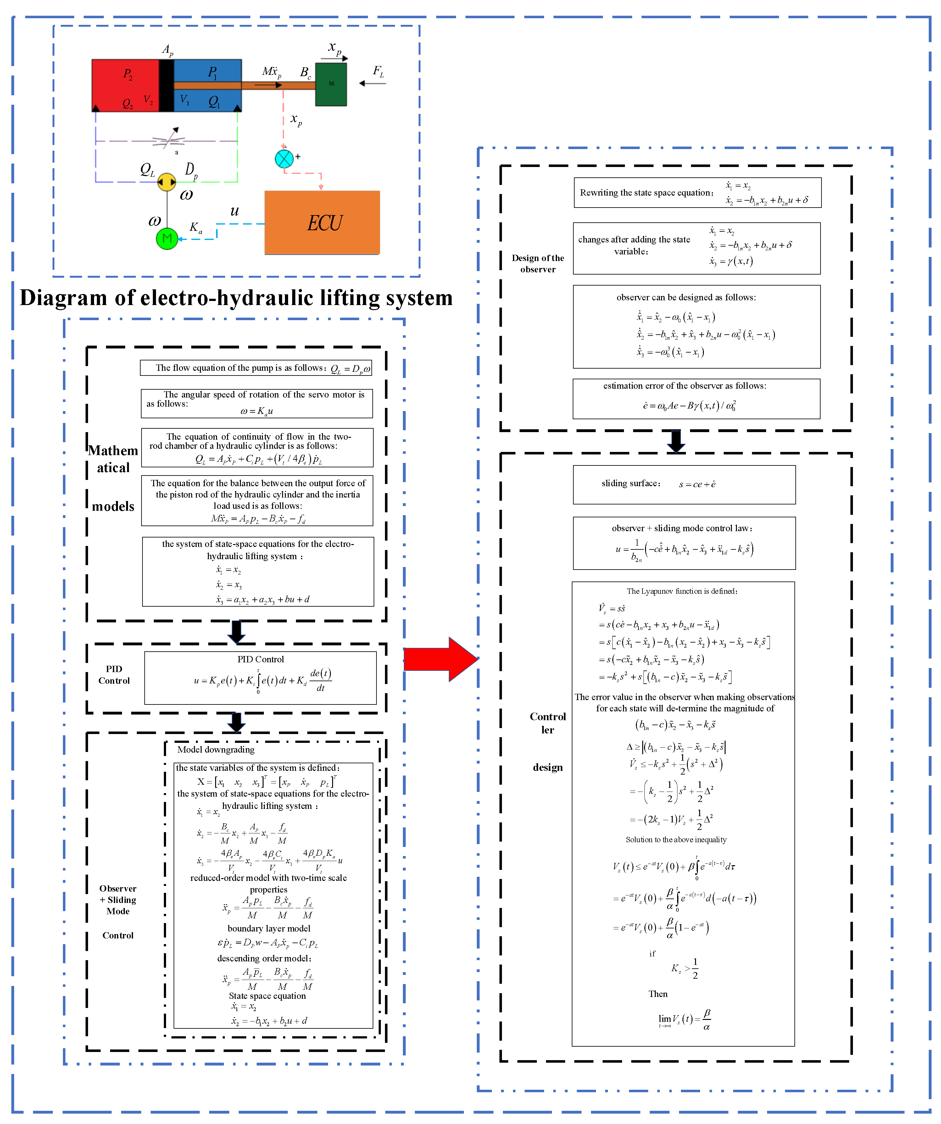
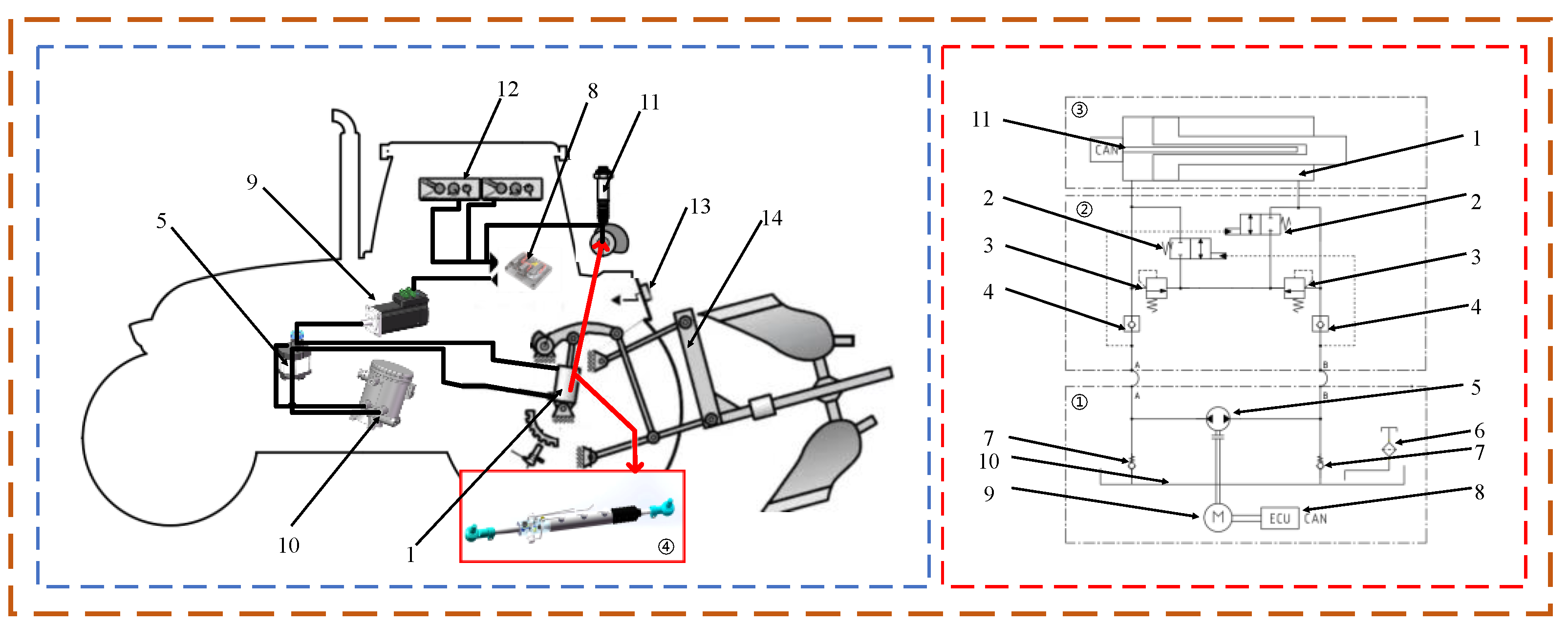
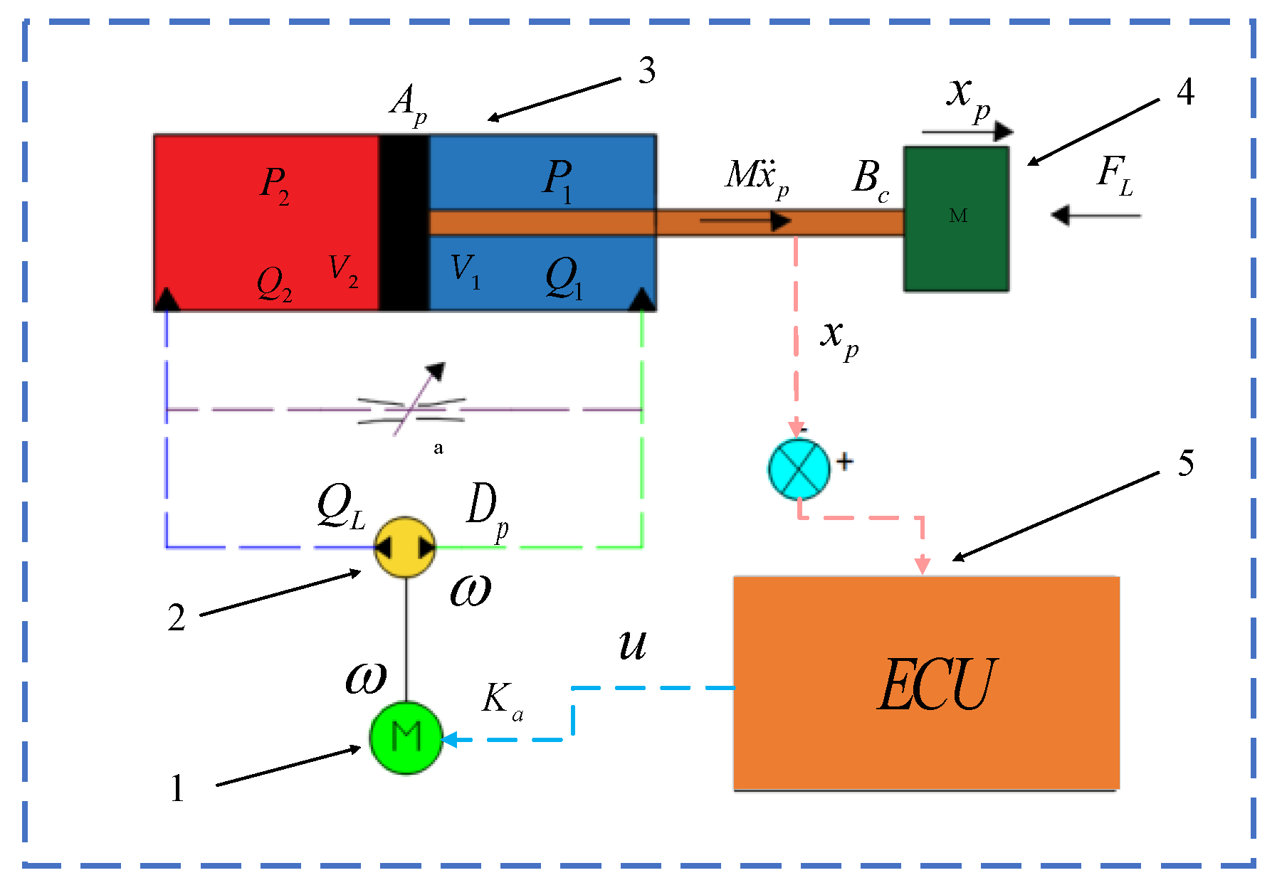
2. Electro-Hydraulic Lifting System Structure and Working Principle

The structure of the tractor electro-hydraulic lifting system is shown in Figure 1. It is mainly composed of the servo motor, dosing pump, hydraulic cylinder, check valve, relief valve, and controller.

Figure 1. Tractor electro-hydraulic lifting device hydraulic schematic. 1—Hydraulic cylinder, 2—Directional valve, 3—Relief valve, 4—One-way valve, 5—Hydraulic pump, 6—Filters, 7—One-way valve with spring, 8—Controller, 9—Motor, 10—Oil tank, 11—Sensors built into hydraulic cylinder, 12—Control panel, 13—Button, 14—Lifting agencies. ①—Power train, ②—Valve train, ③—Executive train, ④—Hydraulic cylinder details.

The electro-hydraulic lifting system uses a closed-loop control scheme in which a servo motor is used as the power unit for the electro-hydraulic lifting system and is connected directly to the gear pump via a coupling. The servo motor controls the gear pump by varying the speed and torque, and the two are combined to achieve control of the system pressure and flow. The thrust and displacement generated by the hydraulic cylinder are controlled by adjusting the magnitude of the system pressure and flow. A relief valve protects the system from pressure overload; the controller collects the status information from the relevant pressure and displacement sensors and outputs control commands to achieve servo control of the hydraulic cylinder.

The purpose of this paper is to design a control strategy to improve the position tracking performance of electro-hydraulic servo system in order to improve the position tracking performance and expand its application range. The working principle is that the tillage depth mode is selected according to the tractor settings, and the ECU transmits the motor signal to the motor. The system uses a servo motor coaxial to drive the dosing pump, and the dosing pump suction and discharge ports are directly connected to the hydraulic cylinder two load oil port relief valve as a safety valve to protect the system pressure from exceeding the safety limit value. The controller outputs the torque and speed command to the servo motor, thus adjusting the output pressure and flow of the dosing pump, and finally realizing the purpose of controlling the output displacement of the hydraulic cylinder piston. The piston rod drives the plough head. The displacement sensor built into the hydraulic cylinder transmits the actual displacement measured by the sensor to the ECU via the CAN bus. The ECU makes a difference between the theoretical displacement and the actual displacement, and the control strategy adjusts it to compensate for the difference in displacement.

3. Mathematical Models and Control Strategy

3.1. Mathematical Models

The mathematical model is built while the following settings are made for the electro-hydraulic lifting system; the hydraulic cylinder has only internal leakage and no external leakage; the hydraulic cylinder load is an inertial load [21]. As shown in Figure 2, the servo motor and hydraulic pump have the same speed. The servo motor drives the hydraulic pump rotation, and the hydraulic cylinder deepens. At this time, the displacement sensor will displace the signal to the ECU, and the ECU will displace the signal into the voltage signal. The servo motor will displace the voltage signal into torque and speed to drive the hydraulic pump.

Figure 2. Mathematical model for electro-hydraulic lifting device. 1—Motor, 2—Hydraulic pump, 3—Hydraulic cylinder, 4—Load, 5—Controller.

Due to the complex structure of the servo motor system and the many non-linear factors, this paper chooses to ignore a part of the complex non-linear factors that are less influential to derive the servo motor mathematical model.

For idealistic reasons, the following assumptions are made for the pump-controlled cylinder system.

① The flow pulsations generated at the output port during the actual operation of the hydraulic pump are not considered.

② Consider the non-linear time-varying parameters in the system (fluid temperature and modulus of elasticity) as constant values.

③ Do not count the flow loss caused by the pressure and resistance along the pipeline during the transmission of the system fluid.

④ The pump-controlled cylinder hydraulic system is a volumetric servo-integrated structure, so there is little flow leakage.

The angular speed of rotation of the servo motor is as follows:

$$\omega =K_{a}u$$

(1)

where: $\omega$ is the angular speed of rotation of the servo motor, $\mathrm{r}\mathrm{a}\mathrm{d}/\mathrm{s}$; $K_a$ is the speed gain, $\mathrm{r}\mathrm{a}\mathrm{d}/\mathrm{s}/\mathrm{V}$; and $u$ is the control voltage input, $\mathrm{V}$.

The output shaft of the servomotor is directly connected to the gear pump via a coupling; thus, the angular speed of rotation of the pump is the same as the output angular speed of the servomotor. The flow equation of the pump is as follows:

$$\left\{\begin{array}{l}{Q}_1=D_p\omega -C_i\left(p_1-p_2\right)\\ Q_2=D_p\omega -C_i\left(p_1-p_2\right)\end{array}\right.$$

(2)

where: $p_1$, $p_2$ are chamber A and B pressures ($\mathrm{pa}$); $Q_1$ is the flow rate in the rod chamber of the hydraulic cylinder (${\mathrm{m}}^3/\mathrm{s}$); $Q_2$ is the flow rate of the rodless chamber of the hydraulic cylinder (${\mathrm{m}}^3/\mathrm{s}$); $C_i$ is the internal leakage coefficient of the quantitative pump $\left({\mathrm{m}}^3/\left(\mathrm{s}\cdot \mathrm{p}\mathrm{a}\right)\right)$; $\omega$ is the input speed $\left(\mathrm{rad}/\mathrm{s}\right)$; $D_p$ is quantitative pump displacement $\left({\mathrm{m}}^3/\mathrm{rad}\right)$.

As the electro-hydraulic lifting system is a non-linearized control system, the first step in the process of building the mathematical model is to linearize the non-linear model. The Rasch transformation is an important tool for solving non-linear problems by which the linearization is carried out. Using the Rasch transformation to solve the system response is relatively intuitive, and it can directly obtain the variations and expressions of the output curve with time.

Organizing Equation (2) after the Rasch transform gives:

$$Q_L=D_p\omega -C_i{P}_L$$

(3)

where: $Q_L$ is the flow equation of the pump, m³/s; $P_L$ is the differential pressure between chambers A and B of the system. $\omega$ is the angular speed of rotation of the pump and motor, rad/s.

The equation of continuity of flow in the two-rod chamber of a hydraulic cylinder is as follows:

$$Q_1=A_p{\dot{x}}_p+C_i\left(p_1-p_2\right)+V_1{\dot{p}}_1/{\beta }_e$$

(4)

$$Q_2=A_p{\dot{x}}_p+C_i\left(p_1-p_2\right)-V_2{\dot{p}}_2/{\beta }_e$$

(5)

where: $Q_1$ is the flow rate in the rod chamber of the hydraulic cylinder, m³/s; $Q_2$ is the flow rate of the rodless chamber of the hydraulic cylinder, m³/s; $A_p$ is the area of the piston rod, ${\mathrm{m}}^2$; $x_p$ is the piston rod displacement, $\mathrm{m}$; $C_i$ is the internal leakage coefficient of the hydraulic cylinder, $\left({\mathrm{m}}^3/\mathrm{s}\right)/\mathrm{P}\mathrm{a}$; $P_1$ and $P_2$ are the pressures in the two chambers of the hydraulic cylinder, $\mathrm{Pa}$; $V_1$ and $V_2$ are the volumes of the two chambers of the hydraulic cylinder, respectively, ${\mathrm{m}}^3$; and ${\beta }_e$ is the bulk modulus of elasticity, $\mathrm{Pa}$.

The load pressure is defined as $P_L=P_1-P_2$, and the load flow is defined as $Q_L=\left(Q_1+Q_2\right)/2$. Thus, combining (3) and (4) gives the following:

$$Q_L=A_P{\dot{x}}_P+C_i{p}_L+\left(V_t/4{\beta }_e\right){\dot{p}}_L$$

(6)

where $V_t$ is the total volume in the hydraulic cylinder chamber, ${\mathrm{m}}^3$.

The equation for the balance between the output force of the piston rod of the hydraulic cylinder and the inertia load used is as follows:

$$M{\ddot{x}}_P=A_P{p}_L-B_c{\dot{x}}_P-f_d$$

(7)

where $M$ is the total mass applied to the piston rod of the hydraulic cylinder, $\mathrm{kg}$; $B_c$ is the viscous damping factor, $\mathrm{N}\cdot \mathrm{s}/\mathrm{m}$; and $f_d$ for items that are difficult to model accurately includes external random disturbance forces and unmodeled friction.

$$x_p=\frac{\frac{D_p{N}_p}{A_p}-\frac{1}{A_p^2}\left(C_i+V_{t}s/4{\beta }_e\right)F_L}{s\left[\frac{s^2}{{\omega }_h^2}+\frac{2{\zeta }_h}{{\omega }_h}s+1\right]}$$

(8)

where: ${\omega }_h$ is the hydraulic inherent frequency, ${\omega }_h=\sqrt{\left(4{\beta }_e{A}_p^2/m_t{V}_t\right)}$; ${\zeta }_h$ is the hydraulic damping ratio, ${\zeta }_h=C_i/A_p\sqrt{\left({\beta }_e{m}_t/V_t\right)}$.

Equation (8) expresses the dynamic response mechanism of the pump-controlled system when subjected to external load disturbances.

According to Equation (8), the position output $x_p$ of the electro-hydraulic lifting system is related to the control speed input, $N_p$, as a function of the following:

$$\frac{x_p}{N_p}=\frac{D_p/A_p}{s\left[\frac{s^2}{{\omega }_h^2}+\frac{2{\zeta }_h}{{\omega }_h}s+1\right]}$$

(9)

The expression structure of Equation (9) is a general formula for the transfer function of pump-controlled hydraulic systems, which is commonly used in various hydraulic servo systems in the research and analysis.

According to Equation (8), the pump control system position output $x_p$ as a function of the external load disturbance input, $F_L$, is as follows as follows:

$$\frac{x_p}{F_L}=\frac{-\frac{1}{A_p^2}\left(C_t+\frac{V_t}{4{\beta }_e}s\right)}{s\left[\frac{s^2}{{\omega }_h^2}+\frac{2{\zeta }_h}{{\omega }_h}s+1\right]}$$

(10)

Combining (1)–(10) and defining the state variables $\mathrm{{\rm X}}={\left[\begin{array}{ccc}{x}_1& x_2& x_3\end{array}\right]}^T={\left[\begin{array}{ccc}{x}_P& {\dot{x}}_P& {\ddot{x}}_P\end{array}\right]}^T$, the system of state-space equations for the electro-hydraulic lifting system is obtained as follows:

$$\begin{array}{l}{\dot{x}}_1=x_2\\ {\dot{x}}_2=x_3\\ {\dot{x}}_3=a_1{x}_2+a_2{x}_3+bu+d\end{array}$$

(11)

where $a_1=\frac{4{\beta }_e{A}_p{}^2+4{\beta }_e{C}_i{B}_c}{V_{t}M}$, $a_2=\frac{4{\beta }_e{C}_{i}M+V_t{B}_c}{V_{t}M}$, $b=\frac{4{\beta }_e{A}_p{D}_p{K}_a}{V_{t}M}$, and $d=-\frac{4{\beta }_e{C}_i}{V_{t}M}{f}_d-\frac{{\dot{f}}_d}{M}$, where the interference $d$ is bounded and satisfies $\left|d\right|\le D$.

3.2. Electro-Hydraulic Lifting System Control Strategy

The tractor’s electro-hydraulic lifting system regulates the lifting system’s attitude using the telescopic movement of the end-effector hydraulic cylinder, thus indirectly controlling the plowing depth. First, the target plowing depth set by the user is transmitted to the controller, whereas the controller reads the value of the position (angle) sensor in real-time to obtain the actual plowing depth. Then, the controller sends the corresponding electrical control command to the controlled element (servo motor) of the hydraulic system through a logic operation to regulate the expansion and contraction of the hydraulic cylinder and finally realize the control of the position of the implements.

3.2.1. Conventional PID Control

The PID controller is a linear controller that controls the control object by linearly combining the proportional (P), integral (I), and differential (D) of the deviation of the given value $U\left(0\right)$ from the actual output value $U\left(t\right)$ to form the control quantity. The control signal input to the system is the deviation of the target signal from the actual signal, and the output of the system is as follows:

$$u=K_{p}e\left(t\right)+K_i{\displaystyle \underset{0}{\overset{t}{\int }}e\left(t\right)dt+K_d\frac{de\left(t\right)}{dt}}$$

(12)

where $u$ is the output of the controller; $e\left(t\right)$ is the deviation signal; $K_p$ is the input to the system; $K_i$ is the proportional amplification factor of the controller; and $K_d$ is the integration factor of the controller.

The transfer function is as follows:

$$G_e\left(S\right)=K_p+K_i\frac{1}{s}+K_{d}s$$

(13)

$K_p$, $K_i$, and $K_d$ act on the system in terms of proportionality, integration, and differentiation, respectively, solving for the appropriate parameters to bring the closed loop system to the desired control effect.

In this paper, the PID parameters are adjusted by means of the Ziegler–Nichols parameter adjustment method.

$$K_p=0.6K_m, K_d=\frac{0.25k_p\pi }{{\omega }_m}, K_i=\frac{K_p{\omega }_m}{\pi }$$

(14)

where $K_m$ is the value of K at the start of the system oscillation, and ${\omega }_m$ is the frequency of oscillation rate. Using the root trajectory method, we obtain $K_m$, ${\omega }_m$.

The most important of these is the determination of the 3 internal parameters of the system, namely the scale factor, the integration time constant, and the differential time constant. The optimal parameters for the speed PID controller and the position PID controller are sought by means of parameter tuning. In this paper, the parameters of the position PID controller with the optimal control effect are chosen as follows: $K_p=4000$, $K_i=20$ and $K_d=0$.

PID control parameters are optimized by using the packaging technique of the NCD Outport function module in the subsystem model library and the NCD Blockset submodule library in Simulink. They are optimized with $K_p=5000$, $K_i=10$, and $K_d=0$.

3.2.2. Observer–Sliding Mode Control

The sliding-mode controller is built on the basis of the higher-order mathematical model of the electro-hydraulic lifting system. In this study, the higher-order mathematical model of the electro-hydraulic lifting system is first reduced to simplify the design process of the controller. As the electro-hydraulic hoisting system of the tractor has some problems such as different soil conditions and random external load disturbance in actual operation, an observer-sliding mode controller is designed for this purpose, and a Lyapunov stability proof of the system is given [22].

(1)

Model downgrading

First, the state variables of the system are defined: $\mathrm{{\rm X}}={\left[\begin{array}{ccc}{x}_1& x_2& x_3\end{array}\right]}^T={\left[\begin{array}{ccc}{x}_P& {\dot{x}}_P& p_L\end{array}\right]}^T$. The system of state space equations can then be obtained by the union of Equations (1)–(10), which is as follows:

$$\begin{array}{l}{\dot{x}}_1=x_2\\ {\dot{x}}_2=-\frac{B_c}{M}{x}_2+\frac{A_P}{M}{x}_3-\frac{f_d}{M}\\ {\dot{x}}_3=-\frac{4{\beta }_e{A}_p}{V_t}{x}_2-\frac{4{\beta }_e{C}_i}{V_t}{x}_3+\frac{4{\beta }_e{D}_p{K}_a}{V_t}u\end{array}$$

(15)

The effects of unmodeled friction and external random disturbance forces on the control performance should also be considered, but Equation (11) shows that compensation for non-matching disturbances in the system is not possible because its input and disturbance are not in the same differential equation [23].

In practical electro-hydraulic lifting systems, $V_t$ is much smaller than ${\beta }_e$. Thus, this study defines the perturbation parameters as $\epsilon =V_t/\left(4{\beta }_e\right)$.

The system model is decomposed into a reduced-order model with two-time scale properties (16) and a boundary layer model (17).

$${\ddot{x}}_p=\frac{A_p{p}_L}{M}-\frac{B_c{\dot{x}}_p}{M}-\frac{f_d}{M}$$

(16)

$$\epsilon {\dot{p}}_L=D_{P}w-A_P{\dot{x}}_p-C_i{p}_L$$

(17)

Let $\epsilon =0$. Equation (17) becomes an algebraic equation:

$$0=D_{p}w-A_p{\dot{x}}_p-C_i{p}_L$$

(18)

From Equation (18), the quasi-steady state ${\overline{p}}_L$ is as follows:

$${\overline{p}}_L=h\left(t,x\right)=\left(D_{p}w-A_p{\dot{x}}_p\right)/C_i$$

(19)

Variable substitution is performed as follows:

$$y=p_L-h\left(t,x\right)$$

(20)

$\tau =t/\epsilon$ is redefined for the time variable as follows:

$$\frac{dy}{d\tau }=\epsilon \frac{dy}{dt}=\epsilon {\dot{p}}_L-\epsilon \dot{h}$$

(21)

From the conjunction of (17), (20), and (21), we obtain the following:

$$\begin{array}{l}\frac{dy}{d\tau }=D_{p}w-A_p{\dot{x}}_p-C_i\left(y+h\right)\\ =D_{p}w-A_p{\dot{x}}_p-C_i\left[y+\left(D_{p}w-A_p{\dot{x}}_p\right)/C_i\right]\\ =-C_{i}y\end{array}$$

(22)

where $C_i$ is the internal leakage coefficient of the hydraulic cylinder and is positive. The boundary had the exponential constant stability of model (15); as shown in Formula (20), the model reduces the order work correctly.

According to Tikhonov’s theorem [24], given any $t_b>0$, ${\epsilon }^{\ast }$ exists such that $t>t_b$. Only $\epsilon <{\epsilon }^{\ast }$; $p_L-h\left(t,x\right)=O\left(\epsilon \right)$ is established.

Thus, the electro-hydraulic lifting system descending order model is as follows:

$${\ddot{x}}_p=\frac{A_p{\overline{p}}_L}{M}-\frac{B_c{\dot{x}}_p}{M}-\frac{f_d}{M}$$

(23)

where ${\overline{p}}_L$ is the quasi-steady state of the load pressure $p_L$.

Define state variables: $\mathrm{{\rm X}}={\left[\begin{array}{cc}{x}_1& x_2\end{array}\right]}^T={\left[\begin{array}{cc}{x}_p& {\dot{x}}_p\end{array}\right]}^T$. Equation (23) can be written in the form of a state space, which is as follows:

$$\begin{array}{l}{\dot{x}}_1=x_2\\ {\dot{x}}_2=-b_1{x}_2+b_{2}u+d\end{array}$$

(24)

where $b_1=\left(A_p^2{C}_i^{-1}+B_c\right)/M, b_2=A_p{D}_p{K}_a/\left(C_{i}M\right), d=f_d/M$.

Equation (24) shows that the control input u and disturbance d fit in the model. The objective is met after the higher order model of the electro-hydraulic lifting system has been downscaled. This study aims to control the output position to track the given desired trajectory as closely as possible by means of a reasonable control law u.

(2)

Controller design

The role of the observer is to estimate the velocity signal of the hydraulic cylinder and solve the problem of missing information on the velocity of the hydraulic cylinder piston during the design of the controller. After downscaling the mathematical model, strong external random disturbances and parameter uncertainties usually occur. This study designs an observer to estimate system disturbances and compensate for them to improve the robustness of the system.

①

Design of the observer [25]:

$M_n$, $B_{cn}$, and $C_{in}$ are nominal values of $M$, $B_c$, and $C_i$, respectively, and $b_{1n}$, $b_{2n}$, $d_n$, $b_{1n}=\left(A_p^2{C}_{in}^{-1}+B_{cn}\right)/M_n$, and $d_n=f_d/M_n$ are redefined, such that $\tilde{\ast }$ is the difference between the nominal and actual values of the parameter: $\tilde{\ast }={\ast }_n-\ast$. Thus, Equation (24) can be rewritten as follows:

$$\begin{array}{l}{\dot{x}}_1=x_2\\ {\dot{x}}_2=-b_{1n}{x}_2+b_{2n}u+\delta \end{array}$$

(25)

where $\delta ={\tilde{b}}_1{x}_2-{\tilde{b}}_{2}u+d$ represents the total disturbance of the system.

To estimate the total perturbation $\delta$ better, this study sets $\delta$ to be differentiable, thus defining $x_3=\delta$ as a state variable of the system. The system then changes after adding the state variable:

$$\begin{array}{l}{\dot{x}}_1=x_2\\ {\dot{x}}_2=-b_{1n}{x}_2+b_{2n}u+\delta \\ {\dot{x}}_3=\gamma \left(x,t\right)\end{array}$$

(26)

where $\gamma \left(x,t\right)$ represents the rate of change of $\delta$.

Let $\widehat{\mathrm{{\rm X}}}=\left[\begin{array}{ccc}{\widehat{x}}_1& {\widehat{x}}_2& {\widehat{x}}_3\end{array}\right]$ be the vector of estimates for state $\mathrm{{\rm X}}=\left[\begin{array}{ccc}{x}_1& x_2& x_3\end{array}\right]$. The observer can be designed as follows:

$$\begin{array}{l}{\dot{\widehat{x}}}_1={\widehat{x}}_2-{\omega }_0\left({\widehat{x}}_1-x_1\right)\\ {\dot{\widehat{x}}}_2=-b_{1n}{\widehat{x}}_2+{\widehat{x}}_3+b_{2n}u-{\omega }_0^2\left({\widehat{x}}_1-x_1\right)\\ {\dot{\widehat{x}}}_3=-{\omega }_0^3\left({\widehat{x}}_1-x_1\right)\end{array}$$

(27)

where ${\omega }_0$ is the bandwidth parameter of the observer.

We define $\widetilde{\mathrm{{\rm X}}}=\widehat{\mathrm{{\rm X}}}-\mathrm{{\rm X}}$; $e=\Lambda \widetilde{\mathrm{{\rm X}}}$ combining (26) with (27) yields the dynamics of the estimation error of the observer as follows:

$$\dot{e}={\omega }_{0}Ae-B\gamma \left(x,t\right)/{\omega }_0^2$$

(28)

where $\Lambda =\left[\begin{array}{ccc}1& 0& 0\\ 0& {\omega }_0^{-1}& 0\\ 0& 0& {\omega }_0^{-2}\end{array}\right]$$A=\left[\begin{array}{ccc}-1& 1& 0\\ -1& -b_{1n}/{\omega }_0& 1\\ -1& 0& 0\end{array}\right]$$B=\left[\begin{array}{c}0\\ 0\\ 1\end{array}\right]$.

For the estimation error of the observer above, the following condition is set: $\gamma \left(x,t\right)$ is bounded. That is, an unknown positive integer ${\gamma }_{\max }$ exists such that $\left|\gamma \left(x,t\right)\right|\le {\gamma }_{\max }$. If the setting condition above holds, then the following corollary exists: $t_1>0$ and ${\omega }_0>0$ at finite time $t_1$, such that, for ${\forall }_t\ge t_1$, $\left|{\tilde{x}}_i\right|\le {\sigma }_i\left(i=1,2,3\right)$, the corollary holds. Furthermore, the error bounds ${\sigma }_i=O\left({\omega }_0^{-m}\right)$ and $m$ are certain suitable positive integers.

The solution to Equation (28) can be expressed as follows:

$$e\left(t\right)=e\left(0\right)e^{{\omega }_{0}At}-{\displaystyle \underset{0}{\overset{t}{\int }}B\frac{\gamma }{{\omega }_0^2}{e}^{{\omega }_{0}A\left(t-\tau \right)}}d\tau$$

(29)

where $e\left(0\right)={\left[\begin{array}{ccc}{e}_1\left(0\right)& e_2\left(0\right)& e_3\left(0\right)\end{array}\right]}^T$ is the initial estimation error vector.

According to the previous setting, $\left|\gamma \left(x,t\right)\right|\le {\gamma }_{\max }$ holds. Then,

$$\begin{array}{l}\left|e_i\left(t\right)\right|\le \left|e_i\left(0\right)e^{{\omega }_{0}At}\right|+\\ \frac{{\gamma }_{\max }}{{\omega }_0^3}\left[{\left|\left(A^{-1}B\right)\right|}_i+\left|{\left(A^{-1}{e}^{{\omega }_{0}At}B\right)}_i\right|\right]\end{array}$$

(30)

where $A^{-1}=\left[\begin{array}{ccc}0& 0& -1\\ 1& 0& -1\\ b_{1n}/{\omega }_0& 1& -\left(b_{1n}+{\omega }_0\right)/{\omega }_0\end{array}\right]$, that ${\left|\left(A^{-1}B\right)\right|}_i\le 1+b_{1n}/{\omega }_0$.

Given that A is Hurwitz [26] (as a positive number), a certain time $t_1$ will make $\left|{\left(e^{{\omega }_{0}At}\right)}_{i,j}\right|\le {\omega }_0^{-1}$, for ${\forall }_t\ge t_1$, $\left|{\left(A^{-1}{e}^{{\omega }_{0}At}B\right)}_i\right|\le \left(3{\omega }_0+b_{1n}\right)/{\omega }_0^2(i,j=1,2,3)$.

In summary,

$$\left|e_i\left(t\right)\right|\le \frac{{\displaystyle \sum \left|e_i\left(0\right)\right|}}{{\omega }_0}+\frac{{\gamma }_{\max }}{{\omega }_0^3}\left(\frac{b_{1n}+{\omega }_0}{{\omega }_0}+\frac{3{\omega }_0+b_{1n}}{{\omega }_0^2}\right)$$

(31)

Given that ${\tilde{x}}_i={\omega }_0^{i-1}{e}_i(i,j=1,2,3)$, Equation (30) is turned into the following:

$$\left|{\tilde{x}}_i\left(t\right)\right|\le {\sigma }_i=\left[\frac{{\displaystyle \sum \left|x_i\left(0\right)\right|}}{{\omega }_0}+{\gamma }_{\max }\left(\frac{1}{{\omega }_0^{4-i}}+\frac{3+b_{1n}}{{\omega }_0^{5-i}}+\frac{b_{1n}}{{\omega }_0^{6-i}}\right)\right]$$

(32)

②

Controller design

In this study, an observer–sliding mode control strategy is used to improve the position-tracking performance of the system.

Defining the position-tracking error as $e=x_1-x_{1d}$, the design sliding surface is as follows:

$$s=ce+\dot{e}$$

(33)

The parameter $c$ is chosen with the precondition that $\lambda +c$ is Hurwitz [18], and the eigenvalues of the polynomial $\lambda +c=0$ contain negative real parts, $c>0$. Taking the derivative with respect to $s$ yields:

$$\begin{array}{l}\dot{s}=c\dot{e^{″}}+\ddot{e}\\ =c\dot{e}+{\dot{x}}_2-{\ddot{x}}_{1\mathrm{d}}\\ =c\dot{e}-b_{1n}{x}_2+x_3+b_{2n}u-{\ddot{x}}_{1d}\end{array}$$

(34)

The observer–sliding mode control law is designed as follows:

$$u=\frac{1}{b_{2n}}\left(-c\widehat{\dot{e}}+b_{1n}{\widehat{x}}_2-{\widehat{x}}_3+{\ddot{x}}_{1d}-k_s\widehat{s}\right)$$

(35)

where $k_s$ is a positive number: $\widehat{\dot{e}}={\widehat{x}}_2-{\dot{x}}_{1d}$, $\widehat{s}=c\widehat{e}+\widehat{\dot{e}}$ and $\widehat{e}={\widehat{x}}_1-x_{1d}$.

The Lyapunov function is defined as $V_s=\frac{1}{2}{s}^2$, then:

$$\begin{array}{l}{\dot{V}}_s=s\dot{s}\\ =s\left(c\dot{e}-b_{1n}{x}_2+x_3+b_{2n}u-{\ddot{x}}_{1d}\right)\\ =s\left[c\left({\dot{x}}_1-{\widehat{x}}_2\right)-b_{1n}\left(x_2-{\widehat{x}}_2\right)+x_3-{\widehat{x}}_3-k_s\widehat{s}\right]\\ =s\left(-c{\tilde{x}}_2+b_{1n}{\tilde{x}}_2-{\tilde{x}}_3-k_s\widehat{s}\right)\\ =-k_s{s}^2+s\left[\left(b_{1n}-c\right){\tilde{x}}_2-{\tilde{x}}_3-k_s\tilde{s}\right]\end{array}$$

(36)

where ${\tilde{x}}_2={\widehat{x}}_2-x_2$, ${\tilde{x}}_3={\widehat{x}}_3-x_3$ and $\tilde{s}=\widehat{s}-s=c{\tilde{x}}_1+{\tilde{x}}_2$.

The error value in the observer when making observations for each state will determine the magnitude of $\left(b_{1n}-c\right){\tilde{x}}_2-{\tilde{x}}_3-k_s\tilde{s}$. In this article, take $\Delta \ge \left|\left(b_{1n}-c\right){\tilde{x}}_2-{\tilde{x}}_3-k_s\tilde{s}\right|$, then:

$$\begin{array}{l}{\dot{V}}_s\le -k_s{s}^2+\frac{1}{2}\left(s^2+{\Delta }^2\right)\\ =-\left(k_s-\frac{1}{2}\right)s^2+\frac{1}{2}{\Delta }^2\\ =-\left(2k_s-1\right)V_s+\frac{1}{2}{\Delta }^2\end{array}$$

(37)

Let $a=2k_s-1$, $\beta =\frac{1}{2}{\Delta }^2$. The solution of ${\dot{V}}_s\le \left(-2k_s-1\right)V_s+\frac{1}{2}{\Delta }^2$ can be expressed as follows:

$$\begin{array}{l}{V}_s\left(t\right)\le e^{-at}{V}_s\left(0\right)+\beta {\displaystyle \underset{0}{\overset{t}{\int }}{e}^{-a\left(t-\tau \right)}}d\tau \\ =e^{-at}{V}_s\left(0\right)+\frac{\beta }{\alpha }{\displaystyle \underset{0}{\overset{t}{\int }}{e}^{-a\left(t-\tau \right)}}d\left(-a\left(t-\tau \right)\right)\\ =e^{-at}{V}_s\left(0\right)+\frac{\beta }{\alpha }\left(1-e^{-at}\right)\end{array}$$

(38)

If $K_s>\frac{1}{2}$, then,

$$\underset{t\to \infty }{\lim }{V}_s\left(t\right)=\frac{\beta }{\alpha }$$

(39)

The stability of the closed-loop system is analyzed by constructing a Lyapunov function, which ensures convergence. The convergence rate depends on the control gain and the observer parameters. The control signal consists of an equivalent sliding mode control term, a robust term, and a disturbance compensation term. The interference compensation term suppresses the uncertainty of the system parameters and the influence of disturbing external forces. The equivalent sliding mode control term is the control function that causes the system state to lie on the surface of the sliding mode, which has an interference-free effect. The electro-hydraulic lifting system can improve its position-tracking performance by combining the three control functions. As shown in Figure 3.

Figure 3. Mathematical models and control strategy.

4. Simulation and Test Studies

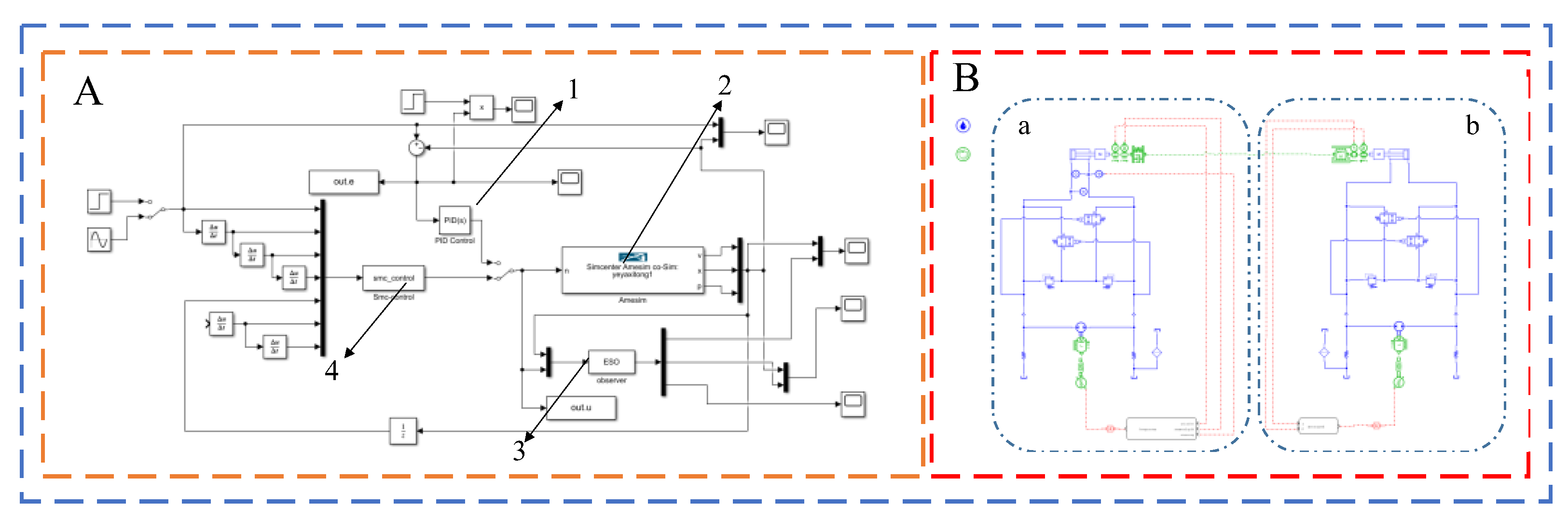
4.1. Simulation and Experimental Principles

The tractor electro-hydraulic lifting control strategy is simulated and verified by means of a step curve and a sinusoidal curve, representing fixed and continuously varying tillage depths, respectively. In the experimental verification, the load resistance cylinder is used to simulate the fixed and continuously varying tillage depth values. In the fixed plowing mode, the displacement sensor of the hydraulic cylinder collects the plowing depth signal, and the difference between the actual plowing depth value and the theoretical target plowing depth value is fed back to the controller, which sends the signal to the servo motor. Then, the servo motor rotates to reduce the difference to 0 further. Based on this, the main purpose of the joint simulation and experimental verification is to verify the response time and accuracy of the process in which the difference was changed to 0 by using different control strategies. The motor is turned forward and reverse to achieve the expansion and contraction of the hydraulic cylinder, which verified the effectiveness of the control strategy utilized in the lowering and lifting process of the tractor electro-hydraulic lifting system. The main purpose of the joint simulation and experimental validation is to verify the difference in response time and accuracy during the process of changing the difference to 0 by using different control strategies, ultimately selecting the optimal control strategy.

In both simulation and practice, the PID mediation process uses the same controller parameters in the displacement control for both Constant load condition and Variable load condition.

4.2. Simulation Studies

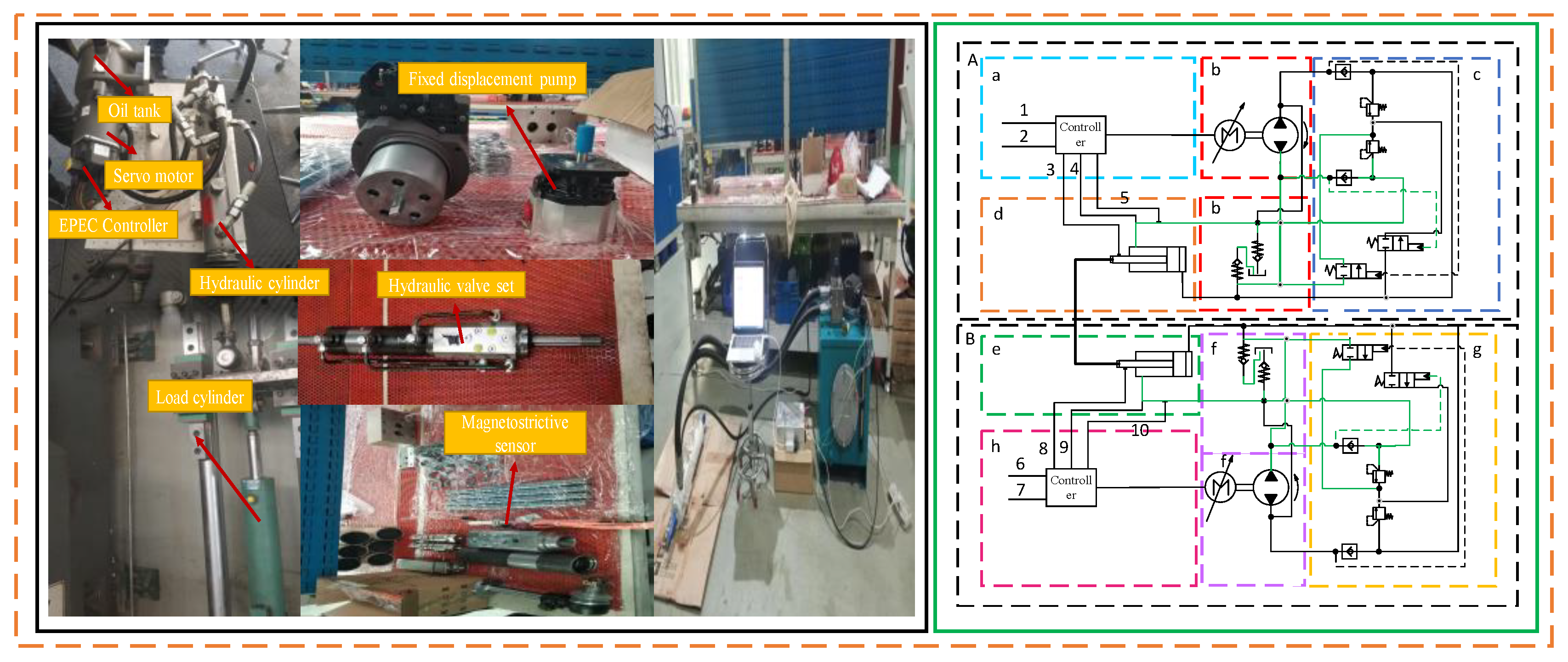
A joint simulation platform is built using MATLAB/Simulink and AMESim to construct a joint simulation model of the electro-hydraulic lifting system. The operation of the electro-hydraulic lifting system is simulated.

Constant load condition: the tractor electro-hydraulic lifting system maintains a constant plowing depth under the same uniform land geology.

Variable load condition: In various land geologies, the tractor’s electro-hydraulic lifting system is switched from a low tillage depth to a high tillage depth rapidly and continuously.

The hydraulic system model in the electro-hydraulic lifting system is built in AMESim. In Figure 4B, a is the electro-hydraulic lifting system, and b is the plowing depth simulation system. A plowing depth simulation with a symmetric structure to the electro-hydraulic lifting system is built in AMESim, which makes the plowing depth simulation system form a symmetry with the electro-hydraulic lifting system. The AMESim simulation model is a left-right symmetric structure with the electro-hydraulic lifting system on the right module and the plowing depth simulation system on the left. The plowing depth simulation system is symmetric to the electro-hydraulic lifting system, which simulates different soil environment resistance depending on the hydraulic cylinder thrust variation. The control effect of the electro-hydraulic lifting system under different resistances provided by the symmetric plowing depth simulation system is verified. The S-function module is created in MATLAB. AMESim creates a MATLAB interface, whose role is to import the hydraulic system model built in AMESim into MATLAB. The input of the interface is the displacement signal x, while the output is the servo motor speed calculated by MATLAB, whereas the observer–sliding mode controller model is built in MATLAB/Simulink. The MATLAB simulation model is shown in Figure 4A. The AMESim model of the hydraulic system is shown in Figure 4B.

Figure 4. Matlab /Simulink and AMESim simulation model. (A)—Matlab simulation module, (B)—AMEsim simulation module, a—Execution module, b—Load simulation module. 1—PID controller, 2—Co-simulation Interface, 3—Extension observer, 4—Sliding mode controller.

As shown in Figure 4A, 1 is the PID controller; 2 is the joint simulation interface; 3 is the observer; 4 is the sliding mode controller. The operational model of the control algorithm of the electro-hydraulic lifting control system can be built in the MATLAB/ Simulink environment. The interface to AMESim can be invoked in Simulink, and the interface file can be generated by compiling the MATLAB interface block in AMESim, and the interface file can be imported into the interface block in Simulink to complete the connection. As shown in Figure 4B, the AMESim hydraulic system model of a variable-amplitude mechanism uses a single-acting hydraulic cylinder model with load, a servo motor model, a quantitative pump model, two sensors for piston rod displacement and pressure measurement, and a proportional gain link for conversion between different unit levels by setting the proportional coefficient. The input to the MATLAB interface is the displacement, speed, and pressure of the piston rod movement, and the output is that of the PID control algorithm, the sliding film control algorithm, and the observer + sliding mode control algorithm, which is output to the servo motor and thus controls the servo action. The simulation parameters are set as shown in Table 1.

Table 1. Basic parameter settings for hydraulic components.

Component Parameters		Numerical
Servo motors	Rated power/kW	2.3
	Rated speed/ (r·min−1)	2300
Dosing gear pumps	Displacement/(cc·r−1)	3
	Rated speed/(r·min−1)	2300
Dosing gear pumps	Bore/mm	50
	Rod diameter/mm	28
	Trips/mm	500
	Coefficient of viscous friction/ (N·(m·s)−1)	1000
	Hydraulic oil density/(kg·m3)	880
	Accumulator volume/L	1
	Relief valve opening pressure/bar	180

In order to verify the effectiveness of parameter optimization in PID control, joint simulations are used to compare and analyze PID control that has not yet been optimized and PID control that has been optimized.

To verify the proposed control strategy, the three control schemes of the observer–sliding mode controller, optimized PID controller, and sliding mode controller are simulated and compared using the joint simulation platform built for the two operating conditions.

4.3. Test Studies

In order to test the accuracy of the proposed control strategy for the electro-hydraulic lifting system of the tractor, validation tests were carried out. Figure 5 shows the test equipment built. In Figure 5, A is an electro-hydraulic lifting system for the application actuator, and B is a plowing depth simulation system, which provides different resistance for A. Similar to the simulation, the semi-physical test stand has a symmetric structure, with the electro-hydraulic lifting system in the upper module and the plowing depth simulation system in the lower module. The plowing depth simulation system, which is symmetric to the electro-hydraulic lifting system, can simulate different soil environmental resistances by using variations in hydraulic cylinder thrusts. The control of the electro-hydraulic lifting system under different operating conditions is verified by means of a semi-physical test rig. The test equipment mainly consists of components such as an EPEC controller, a hydraulic cylinder with magnetostrictive sensors built-in, an integrated valve train, a servo motor, a dosing pump, and an oil tank. During the control process, different control strategies are input via the EPEC controller. Firstly, the displacement of the hydraulic cylinder is measured by a magneto strictive sensor. Secondly, the pressure sensor is mounted on the end chamber of the cylinder head to measure the pressure. In addition, finally, a flow meter is mounted on the hydraulic pump outlet to measure the flow. The EPEC controller is used to collect the above test data.

Figure 5. Diagram of the test stand. A—Execution mechanics, B—Load mechanics, a—Control unit b—Power unit, c—Valve block unit, d—Hydraulic cylinder, e—Hydraulic cylinder in Load mechanics, f—Power unit in Load mechanics, g—Valve block unit in Load mechanics, h—Control unit in Load mechanics. 1—Command signals, 2—Power, 3—Current feedback, 4—Pressure feedback, 5—Displacement feedback, 6—Command signals in Load mechanics, 7—Power in Load mechanics, 8—Current feedback in Load mechanics, 9—Pressure feedback in Load mechanics, 10—Displacement feedback in Load mechanics.

In the test studies, the magnetostrictive displacement sensor collects the displacement of the hydraulic cylinder and transmits the actual displacement to the EPEC controller via the CAN bus. In the controller, the difference between the target displacement and the actual displacement is made, and the displacement signal is converted into a voltage signal recognized by the servo motor, and, through the control strategy proposed above, the servo motor rotation is adjusted according to the displacement difference. The technical parameters of the displacement transducer are shown in Table 2, the technical parameters of the flow meter in Table 3, and the technical parameters of the pressure transducer in Table 4.

Table 2. Technical parameters of the displacement transducer.

Component Parameters	Numerical
Power supply	24VDC
Displacement range	800 mm
Linearity error	10 μm
Update time	0.5 ms
Responsive	1 mm/s
Working temperature	−40 °C–80 °C
Repetition error	2 μm
Output signal	CAN

Table 3. Technical parameters of the flow meter.

Component Parameters	Numerical
Measurement range	0–10 L/min
Precision	0.01 L/min
Responsive	80 ms
Hysteresis	10 mL/min
Working mode	Instantaneous flow
Average display time	0.05 s

Table 4. Technical parameters of the pressure transducer.

Component Parameters	Numerical
Measurement range	−0.1~+10.0 MP
Precision	0.02 Mpa
Responsive	2 ms
Working temperature	−20 °C~+80 °C

5. Results

5.1. Analysis under Constant Load Conditions

5.1.1. PID Parameter Optimization Analysis under Constant Load Conditions

In many engineering applications, PID control parameters are optimized to improve the stability and accuracy of control systems. In this paper, we use joint simulations to verify the correctness of the PID control parameters optimization proposed above under constant load. As shown in Figure 6, the control effect of the conventional PID control and that of the optimized PID control in the displacement control mode are compared. As shown in Figure 7, the control effect of the conventional PID control and that of the optimized PID control in the pressure control mode are compared.

Figure 6. PID control in displacement mode compared with optimized PID control.

Figure 7. PID control in pressure mode compared with optimized PID control.

As shown in Figure 6, without optimizing the PID control parameters, the system reaches the target value at 3.51 s. After parameter optimization, the system reaches the target value at 2.35 s, an improvement of 1.16 S and 33% over the response time of the PID control that is not optimized.

As shown in Figure 7, without optimization of the PID control parameters, the system pressure reaches the target pressure value at 2.35 s. After parameter optimization, the system has fluctuations with a peak value of 52.347 bar from 1.96 s to 2.03 s, and then quickly plateaus and finally reaches the target displacement value at 2.22 s, 0.13 S quicker than the response time of the not yet optimized PID control, which is an improvement of 5%.

After the above verification, the optimized PID control is superior to the conventional PID. In the next work, the optimized PID control will be analyzed in comparison with the proposed control strategy.

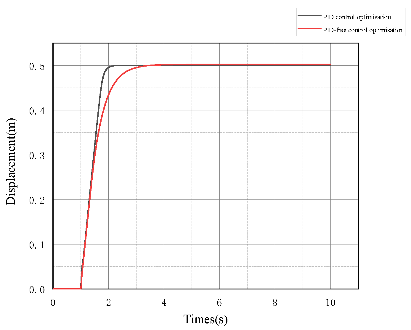
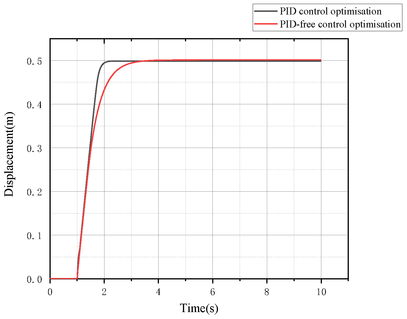
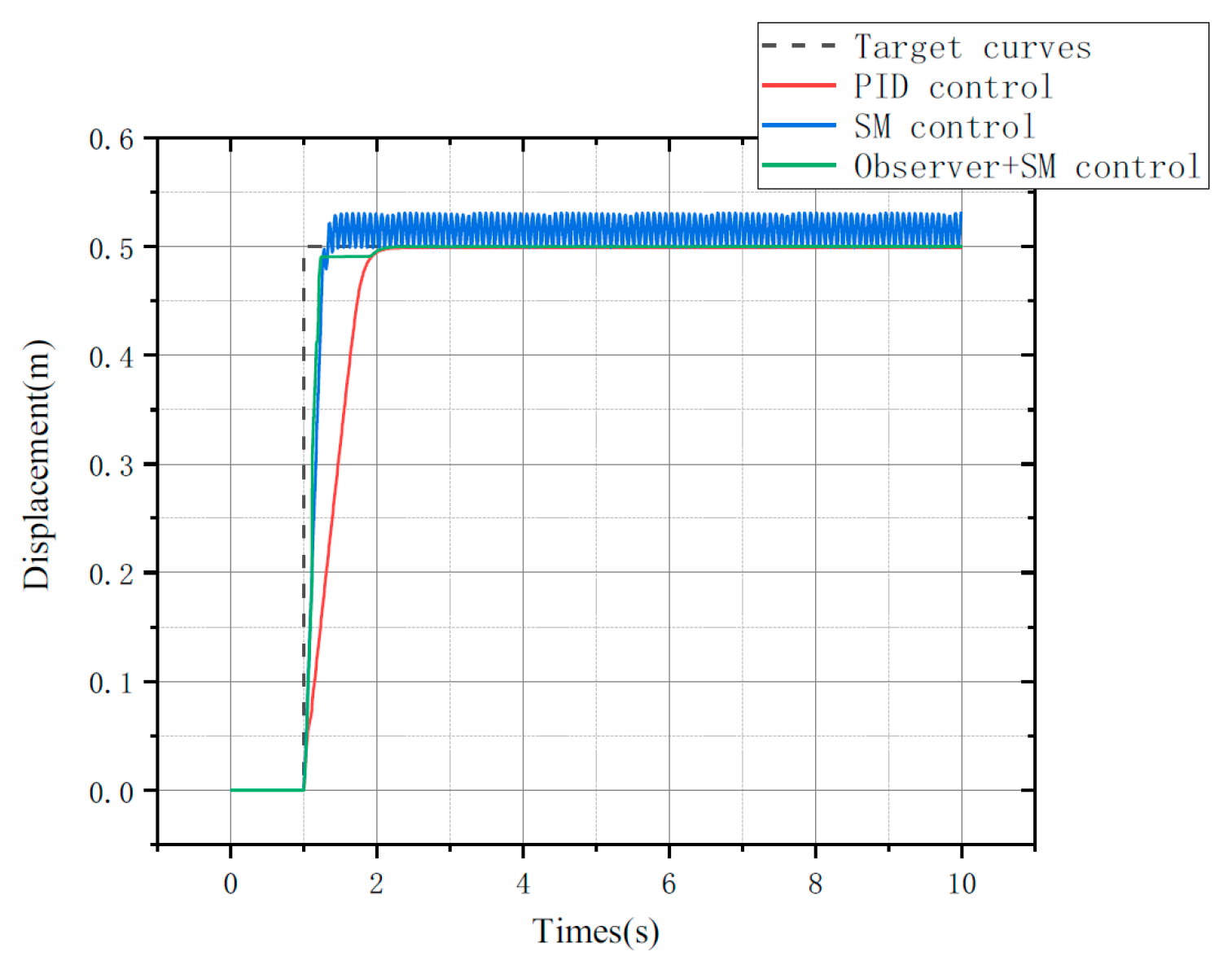
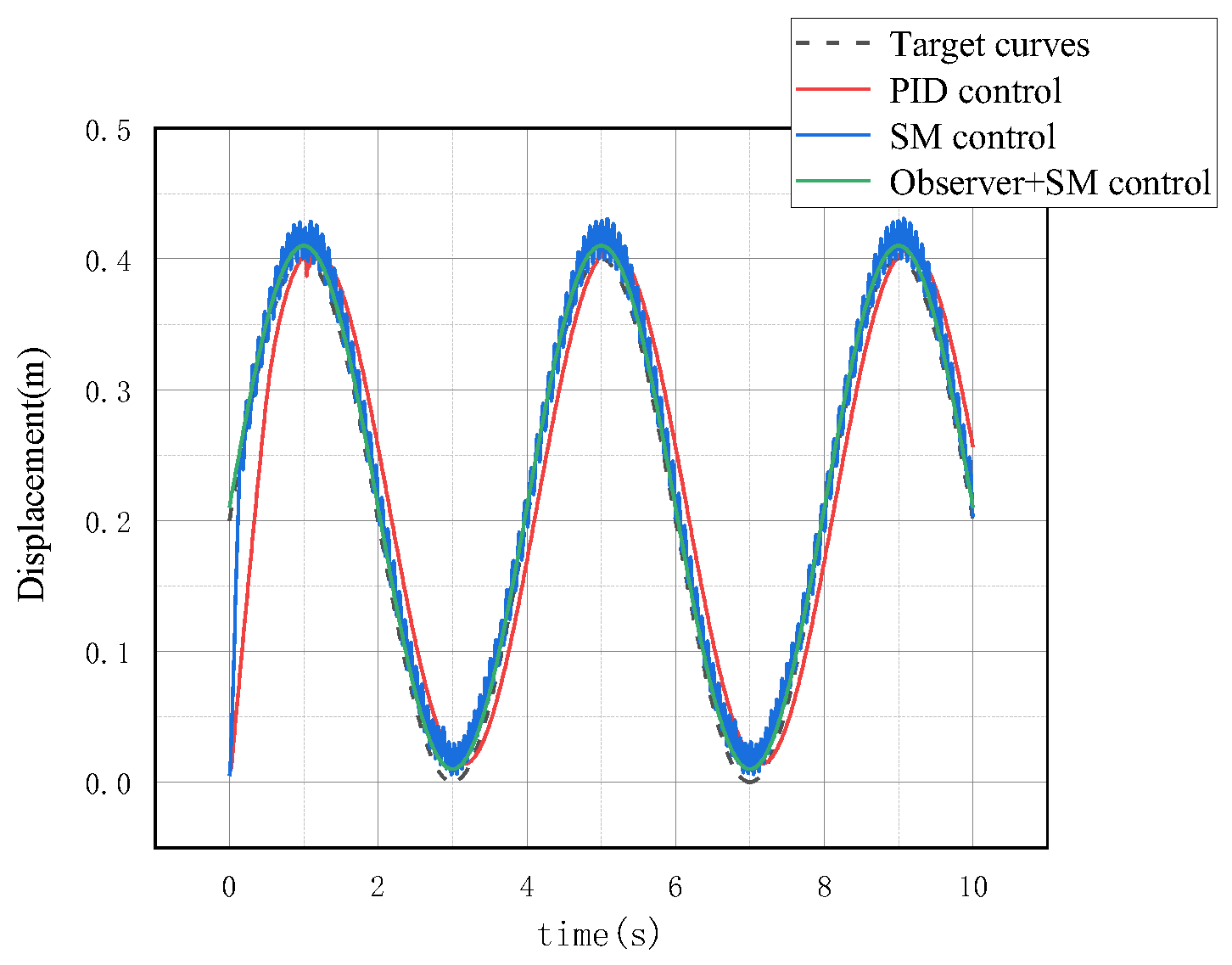
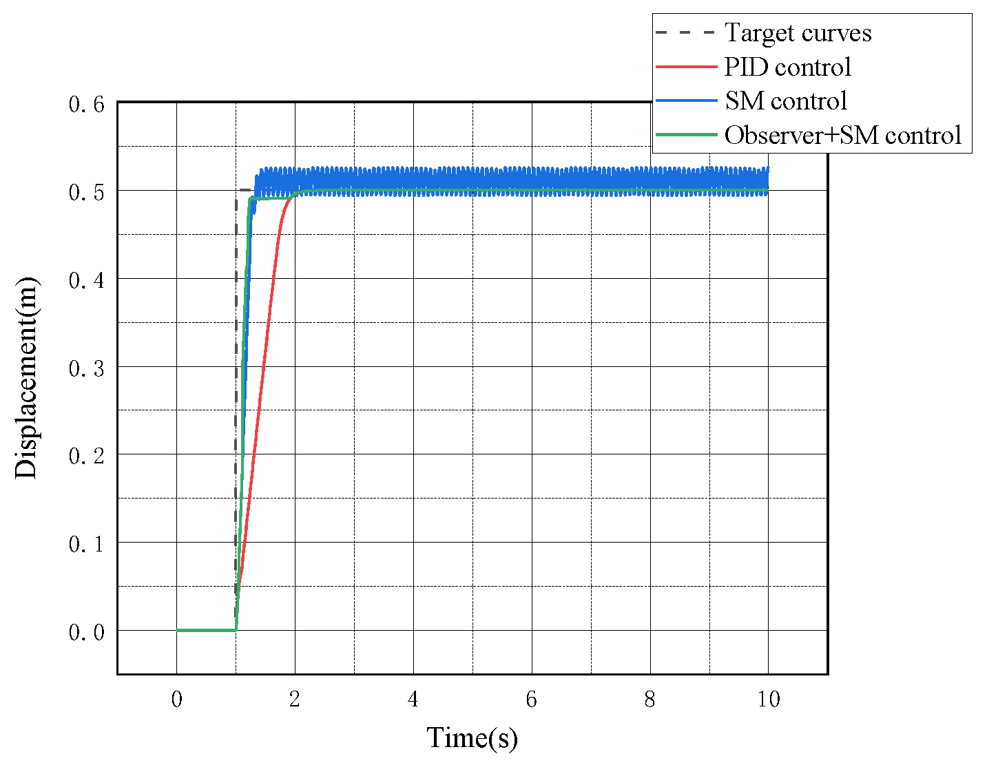
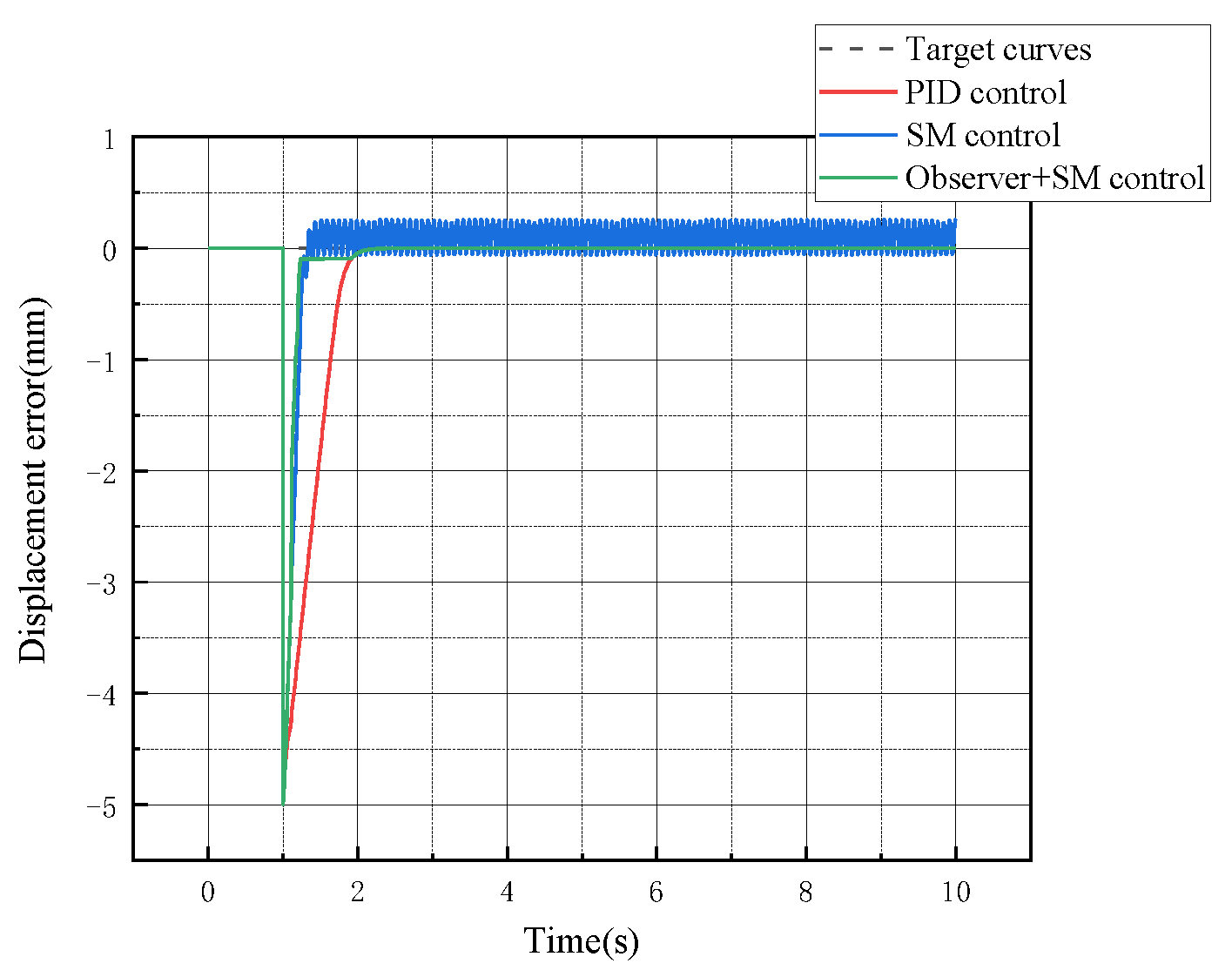
5.1.2. System Displacement Curve Analysis

In this control mode, the system keeps the implement at a constant tillage depth in all soil conditions. Based on this, the constant plowing depth is set to a hydraulic cylinder load of 200 kg. The plowing depth of the realistic tractor electro-hydraulic lifting system is rapidly switched from 0 m to 0.5 m, and the plowing depth of 0.5 m is continuously maintained. The input signal of the simulation system is a 0–0.5 m step signal. The theoretical curve of the hydraulic cylinder displacement, the displacement curve under PID control, the sliding mode control, and the observer–sliding mode control are compared. The displacement curves are compared, and the comparison curves are shown in Figure 8.

Figure 8. Comparison of hydraulic cylinder displacement curves under constant load conditions.

Figure 8 shows that the response speed of PID control is 1.89 s, which is slightly lower than the response speed of 1 s of the desired curve, and the response speed of sliding mode control is 1.32 s. However, the phenomenon of jitter vibration exists in the sliding mode control. Given the jitter phenomenon of the sliding film control, an observer–sliding mode control is designed. The response speed of the observer–sliding mode control is 1.25 s, and the jitter phenomenon of the sliding mode control is effectively solved. The response speed is faster and more accurate than other control strategies.

The displacement error curves of the actual displacement and the desired displacement for the three control methods are shown in Figure 9.

Figure 9. System displacement error under constant load conditions.

As shown in Figure 9, the PID control method has a certain pressure hysteresis when following the steep curve, and the error is large, reaching about 0.48 mm. The error of the sliding mode control method is maintained within 0.3 mm, and its steady state has an obvious jittering phenomenon afterward. The maximum error of the observer–sliding mode control method is 0.5 mm. However, after the steady state, the error can be stabilized within 0.03 mm, and the jitter phenomenon is significantly reduced. The steady-state accuracy of the displacement control under step response is significantly improved using the observer–sliding mode control method.

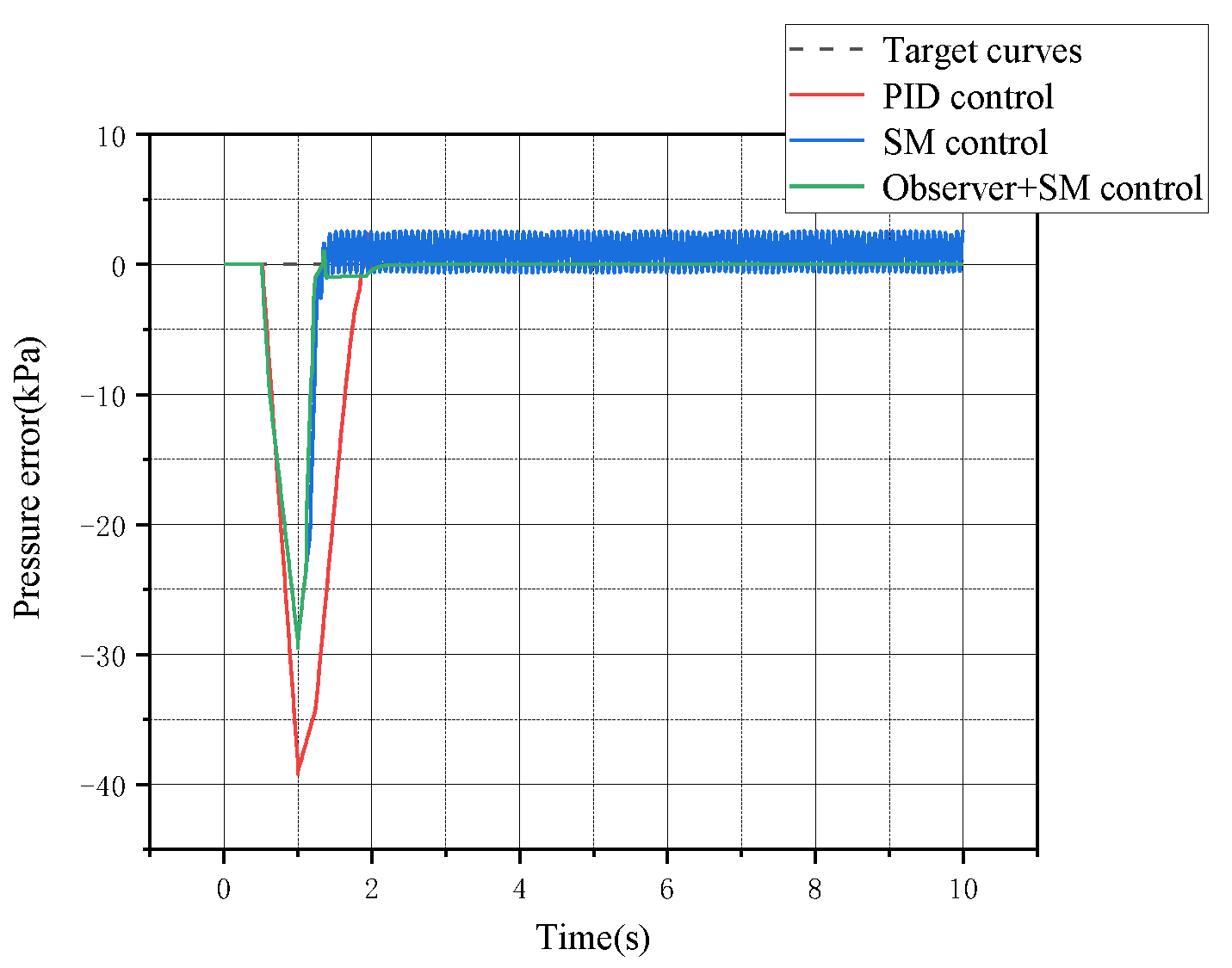
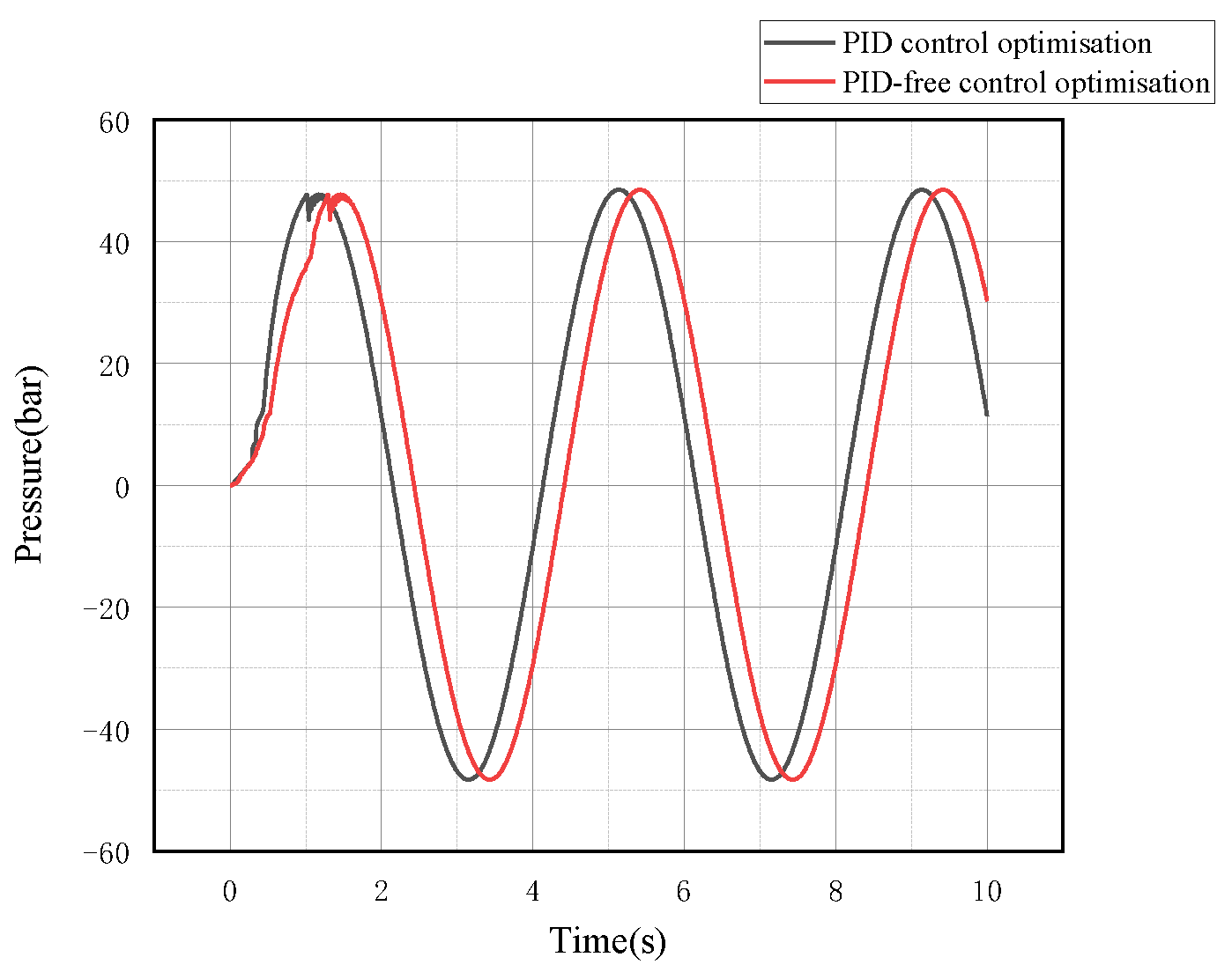
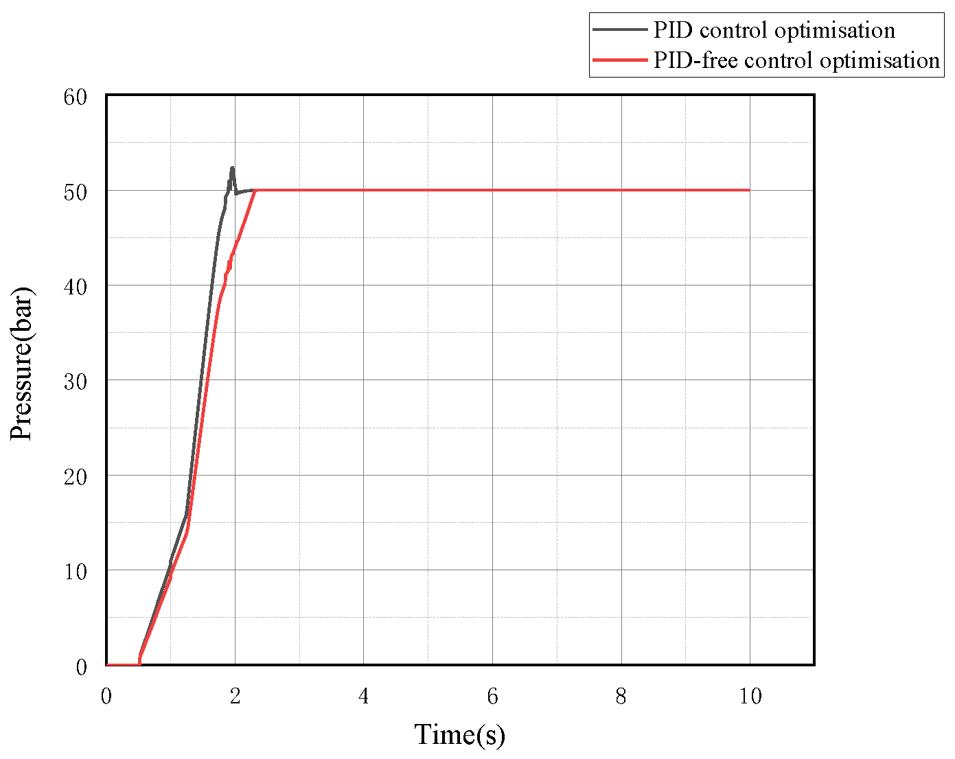
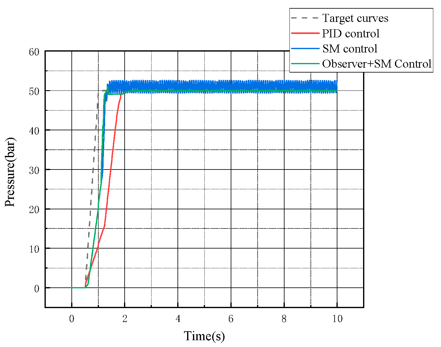
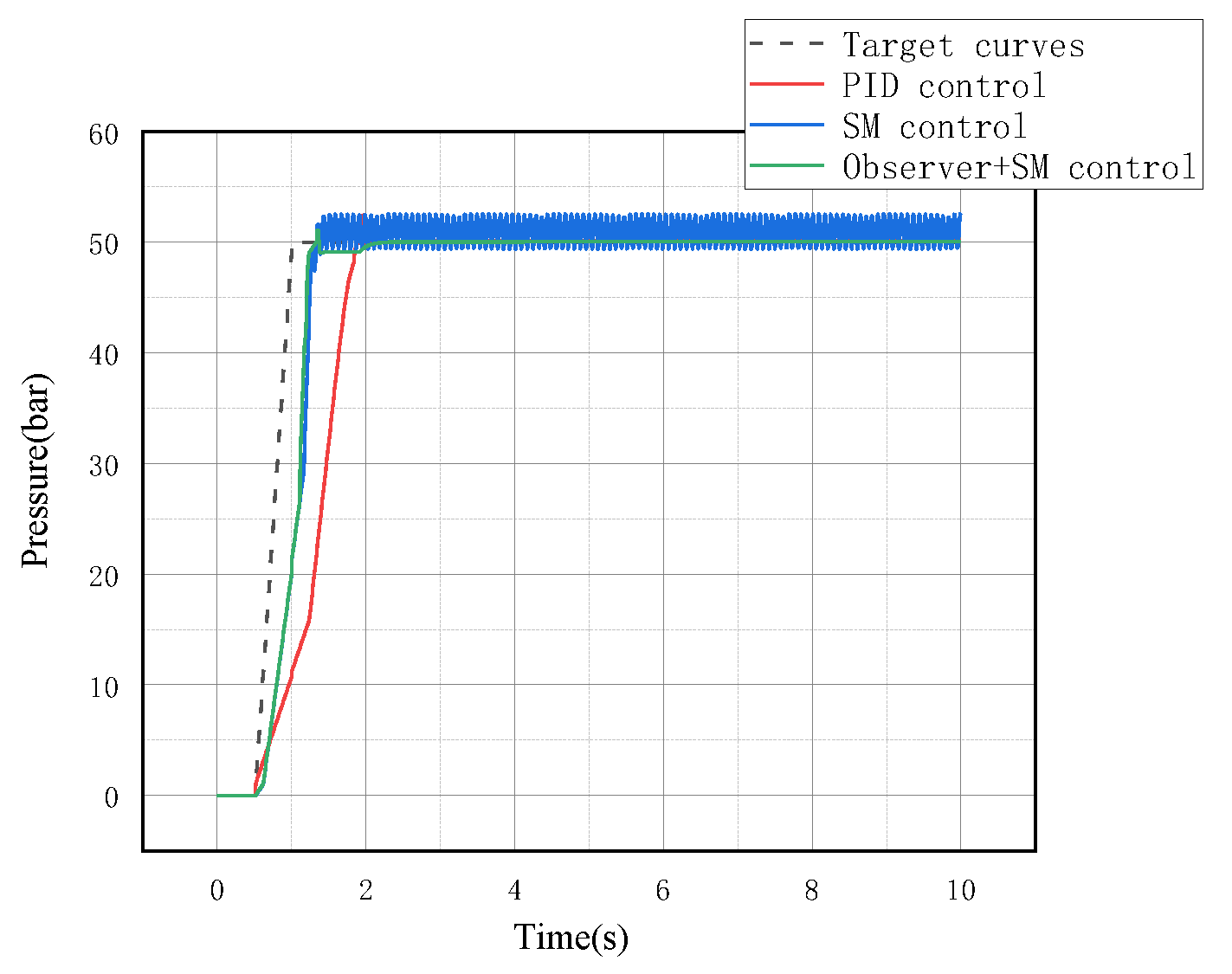
5.1.3. System Pressure Curve Analysis

The above-mentioned fixed plowing depth is set to a hydraulic cylinder load of 200 kg. A realistic tractor electro-hydraulic lifting system has a plowing depth of 0 m to 0.5 m; it rapidly switches and continuously maintains a plowing depth of 0.5 m. The system is represented as the input signal of the simulation system as a 0–0.5 m step signal. Along with the change in displacement signals, the system pressure detection value of the electro-hydraulic lifting system also changes signals. The actual pressure and desired pressure following the process under the PID control are observed, namely sliding film control and observer–sliding mode control methods, as shown in Figure 10.

Figure 10. Comparison of system pressure curves under constant load conditions.

The dynamic response of the PID control, sliding mode control, and observer–sliding mode control methods can be seen in Figure 8. The response speed is 1.89 s with classical PID control, which is slower than 1.53 s for sliding mode control and 1.32 s for observer–sliding mode control. However, the sliding mode control has the phenomenon of jitter and vibration, which cause pressure instability. The observer–sliding mode control method has the response speed of the sliding mode control and can solve the unstable situation of the sliding mode control.

The pressure error curves of the actual pressure and the desired pressure using the three control methods are shown in Figure 11.

Figure 11. System pressure error under constant load conditions.

As shown in Figure 11, the maximum pressure error of the PID control reaches a maximum value of −38.745 kPa at 1.12 s and then increases rapidly and finally stabilizes at −2.014 kPa at 2.15 s. The maximum pressure error of the sliding mode control occurs at 1.31 s, when the pressure error value is −28.54 kPa, and then rises rapidly at 1.56 s and oscillates between 3.4 kPa. The maximum pressure error of −29.45 kPa is reached at 0.94 s with the observer–sliding mode control method and rises quickly at 1.4 s to stabilize at 1.2 kPa.

After a comparative analysis, the steady-state accuracy of pressure control is significantly improved using the observer–sliding mode control method.

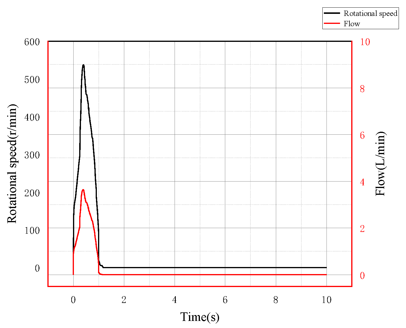
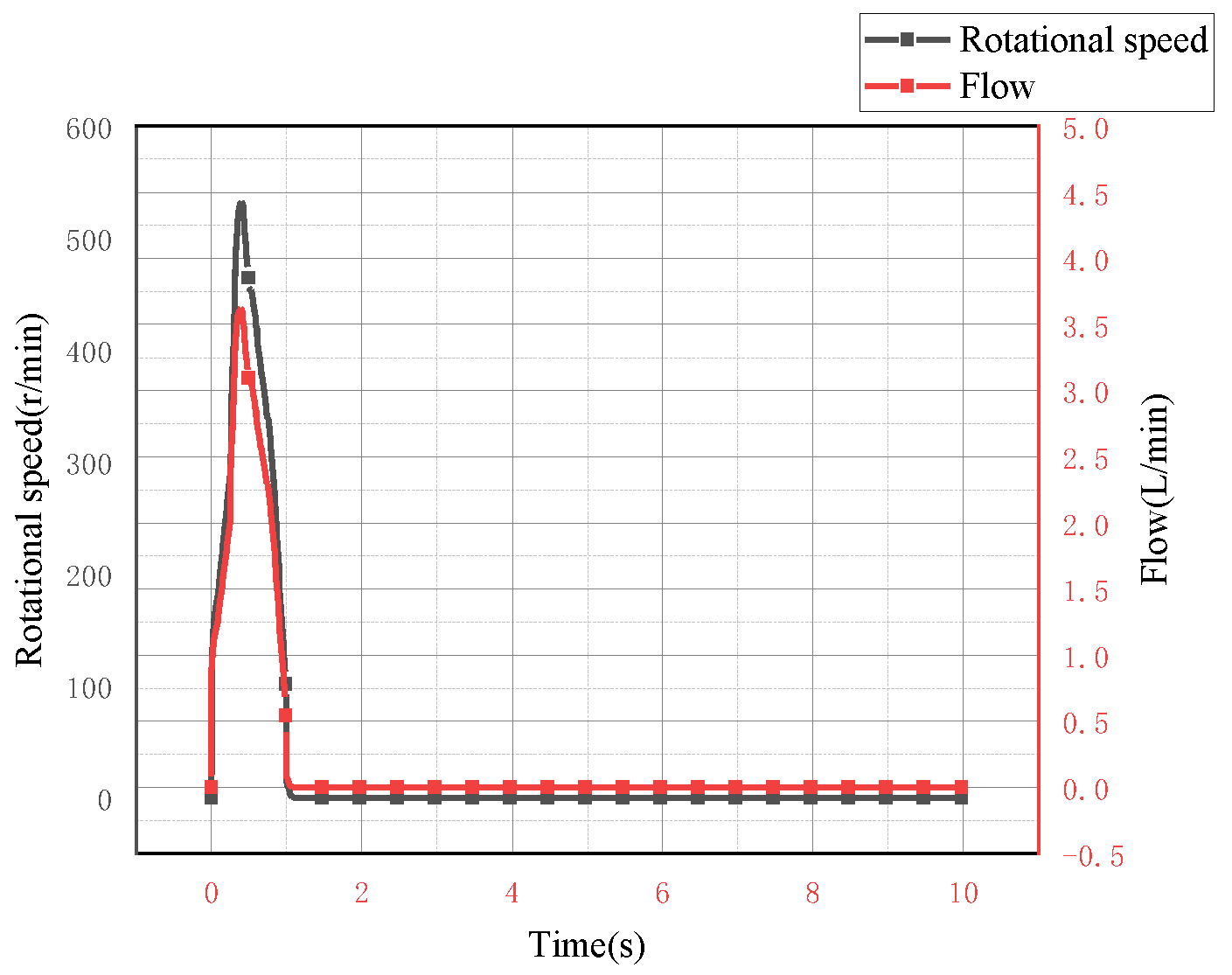
5.1.4. System Speed and Flow Analysis

When using the observer–sliding mode control, the process of changing the speed of the control object servo motor and the system’s flow rate is observed, as shown in Figure 12.

Figure 12. Speed-flow curve under constant load conditions.

Figure 12 shows that the servomotor reaches its peak speed of 545 r/min at 0.5 s and then decreases rapidly (the system flow rate is 3.6 L/min at this point). After 1.32 s, the servomotor stops, and the system flow rate is 0 L/min, with the system reaching a stable plowing depth position. The servomotor speed and flow rate trends are the same. Therefore, the observer–sliding mode control method has a significantly higher response rate.

5.2. Analysis under Variable Load Conditions

5.2.1. PID Parameter Optimization Analysis in Variable Load Conditions

The advanced nature of the optimized PID control compared with conventional PID control is verified. Under the same conditions, the load conditions are variable. As shown in Figure 13, the responsiveness of the conventional PID control and that of the optimized PID control in the displacement control mode are compared under the Variable load condition. As shown in Figure 14, the responsiveness of conventional PID control and that of the optimized PID control in the pressure control mode are compared under the Variable load condition.

Figure 13. PID control in displacement mode compared with optimized PID control.

Figure 14. PID control in pressure mode compared with optimized PID control.

As shown in Figure 13, without optimizing the PID control parameters, the system runs for one cycle at 3.48 s and reaches the target peak at 1.48 s. After parameter optimization, the system runs for one cycle at 3.15 s and reaches the target peak at 1.15 s. After analysis, the one-cycle running time is improved by 0.33 s, and efficiency is increased by 9.48% compared with the PID control that is not optimized; the target peak time is improved by 0.33 s, and efficiency is increased by 22.3%.

As shown in Figure 14, without optimizing the PID control parameters, the system runs for one cycle at 4.42 s and reaches the target peak at 1.45 s. After parameter optimization, the system runs for one cycle at 4.14 s and reaches the target peak at 1.19 s. After analysis, the one-cycle running time is improved by 0.28 s, and efficiency is increased by 6% compared with the PID control that is not optimized; the target peak time is improved by 0.26 s, and efficiency is increased by 17.9%.

After the above verification, the optimized PID control is superior to the conventional PID. In the next work, the optimized PID control will be analyzed in comparison with the proposed control strategy.

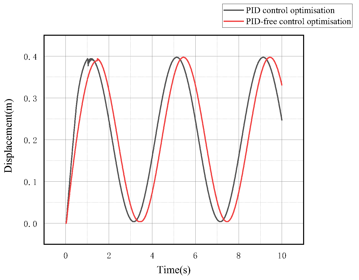
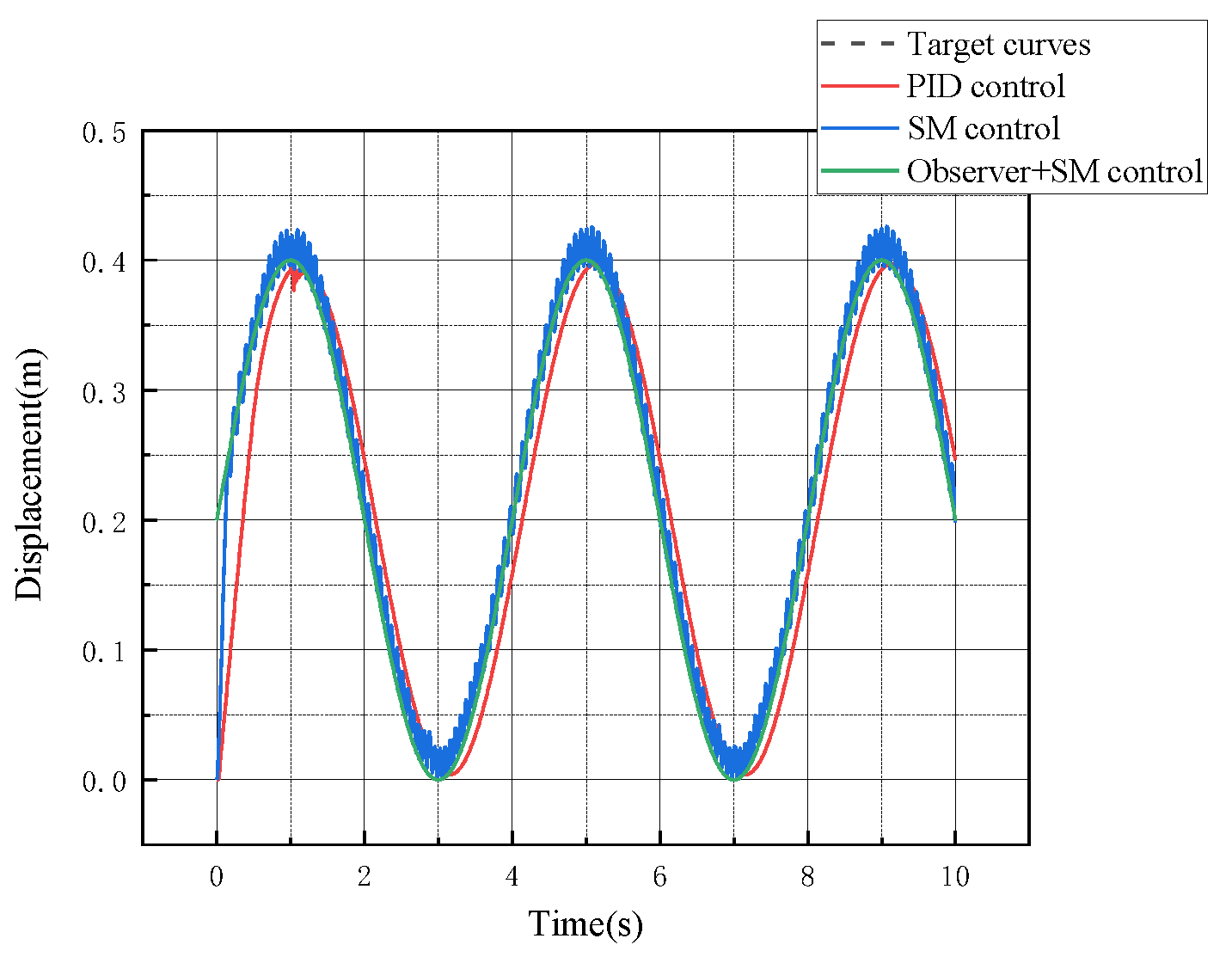
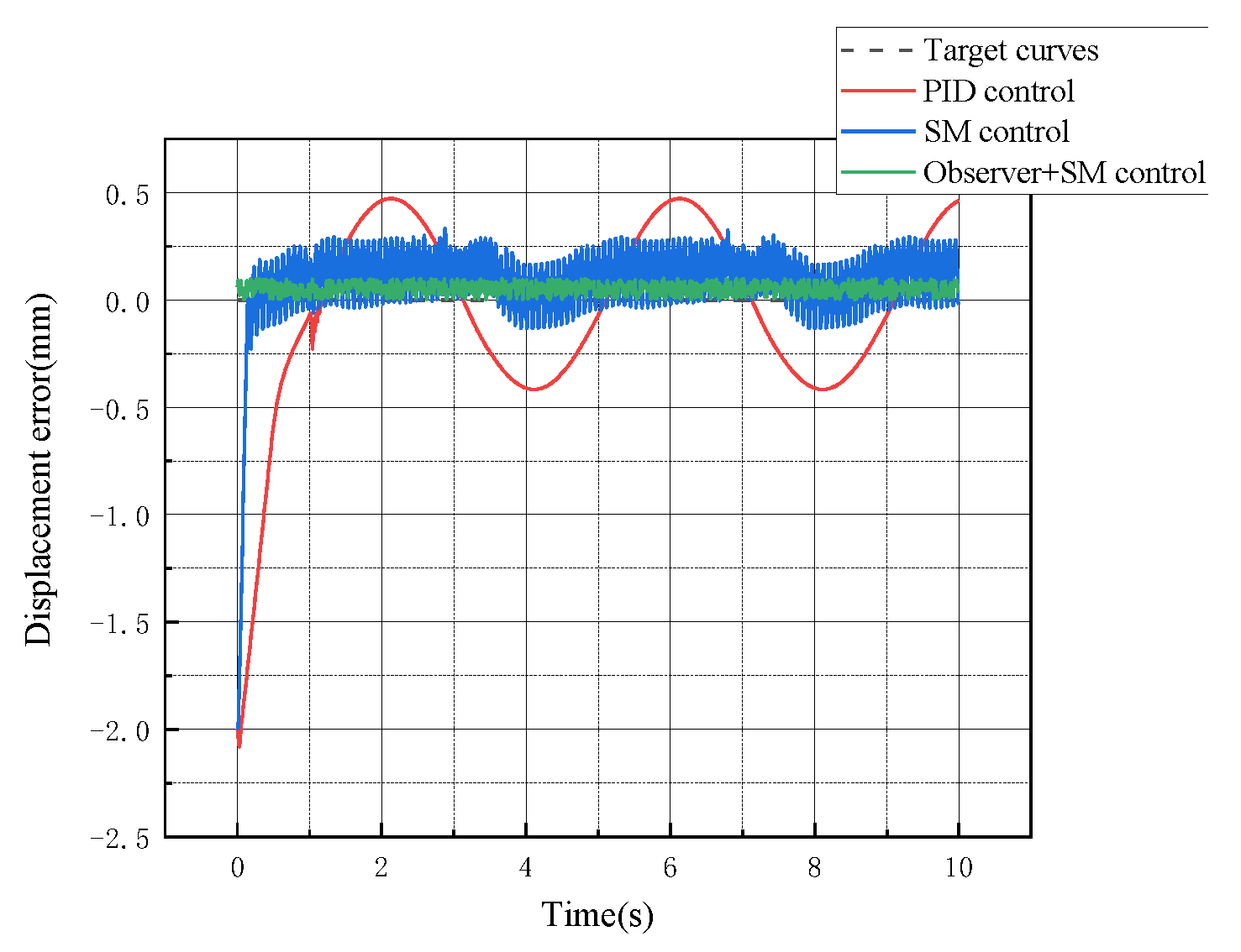
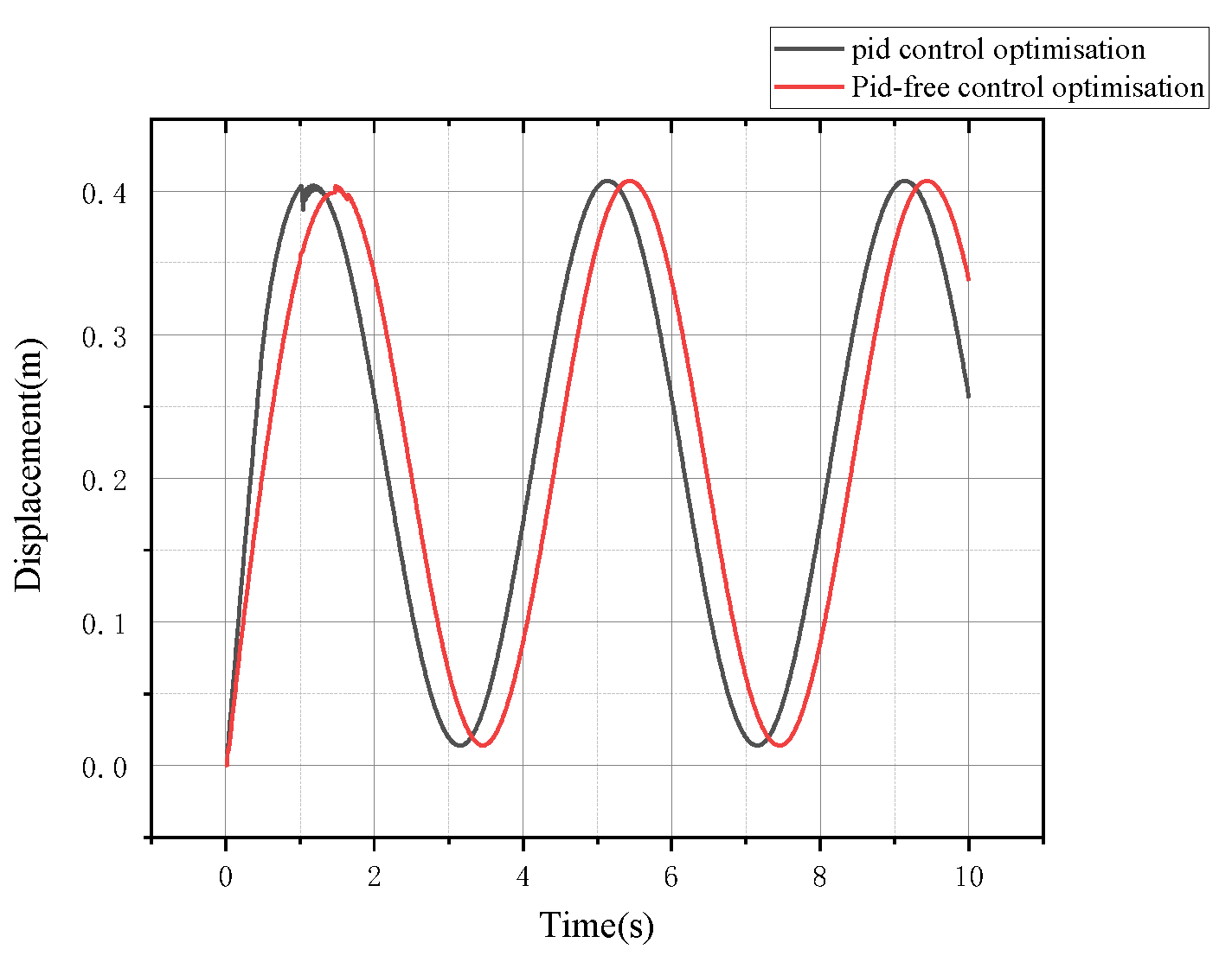
5.2.2. System Displacement Curve Analysis

The electro-hydraulic lifting system commands to the controller based on a different soil geology and different plowing depth values. In response to the above problems, this study selects the hydraulic cylinder load with the form of variable load, which is simulated in the case of different soil, to verify the control effect and control accuracy of the electro-hydraulic lifting system using PID control, sliding mode control, and observer–sliding mode control. The specific condition set in this study is that the tractor application scenario is arable land with a different soil geology. In the joint simulation process, the simulation environment is set to the system input frequency of 0.25 Hz and the amplitude of 200 mm sinusoidal signal as the input signal. The theoretical curve of hydraulic cylinder displacement, the displacement curve under PID control, the displacement curve under sliding mode control, and the displacement curve under observer–sliding mode control are observed for comparison, as shown in Figure 15.

Figure 15. Comparison of hydraulic cylinder displacement curves under variable load conditions.

Figure 15 shows that, under variable load conditions, the tracking effect and response frequency of the electro-hydraulic lifting system using the observer–sliding mode control is significantly better than the PID control strategy and can solve the jitter and vibration phenomenon existing in the single slide film control. The observer–sliding mode control strategy can meet the dynamic and static performance and ensure the stiffness and robustness of the system.

As shown in Figure 16, the PID control method has a certain pressure lag following a sinusoidal curve, and the error is large, reaching 0.25 mm. The error of the sliding mode control method is maintained within 0.22 mm, and it has an obvious jittering phenomenon after the steady state. The maximum error of the observer–sliding mode control method is 0.02 mm, and the jitter phenomenon is significantly reduced. The steady-state accuracy of displacement control under the sinusoidal response is significantly improved by the observer–sliding mode control method.

Figure 16. System displacement error under variable load conditions.

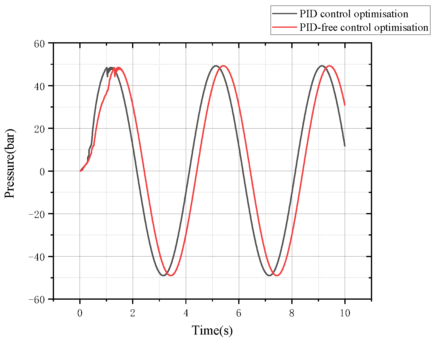
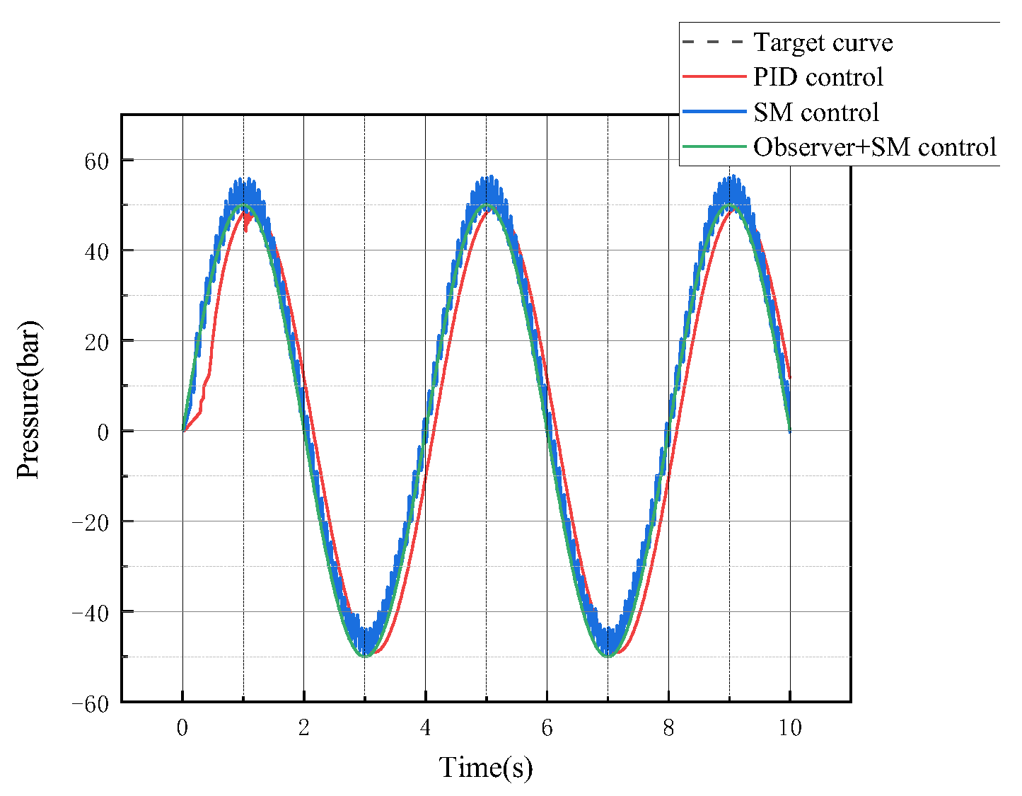
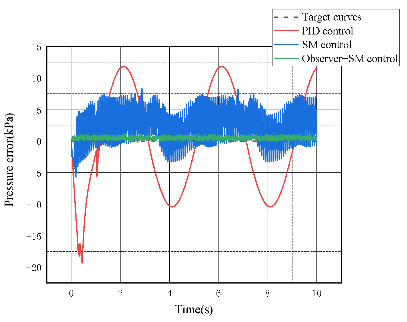
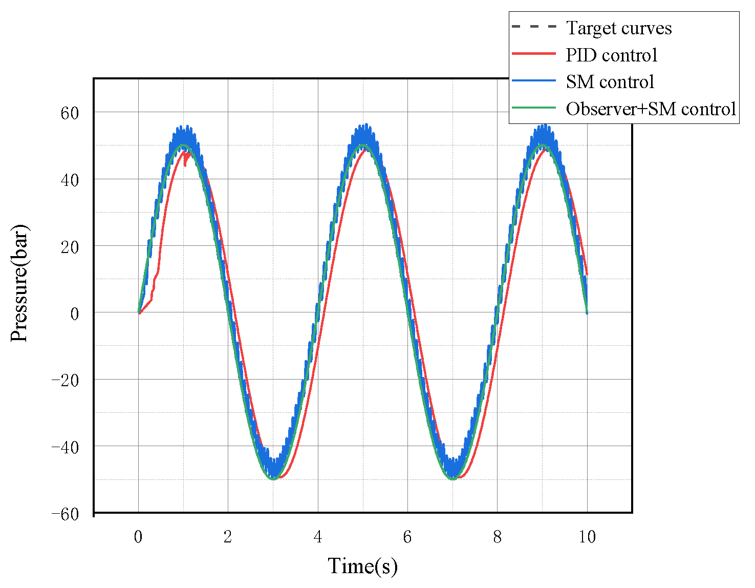
5.2.3. System Pressure Curve Analysis

According to the displacement curve of the hydraulic cylinder under variable load conditions above, the pressure variation of the electro-hydraulic lifting system under the PID control, sliding mode control, and observer–sliding mode control methods is observed analytically, as shown in Figure 17.

Figure 17. Comparison of system pressure curves under variable load conditions.

In Figure 17, the system pressure increases with the increasing displacement. The maximum value is at 52 bar. The response speed under PID control is slower than the others, whereas the response speed under sliding mode control is faster but shows an oscillation phenomenon. The response speed under observer–sliding mode control is the fastest and shows no oscillation phenomenon. Compared with the classical PID control and sliding mode control methods, the observer–sliding mode control method has better response characteristics when following the pressure profile under variable load conditions [27].

As shown in Figure 18, the system pressure error under variable load conditions has a maximum value of −19.3 kPa under PID control and tends to be sinusoidal after 1 s, fluctuating between 12 kPa and −10.5 kPa. The system pressure error curve under sliding mode control also has irregular dithering between 7.7 kPa and −3 kPa because of the dithering nature of the system pressure curve. The system pressure error curve under the observer–sliding mode control is significantly reduced compared with the other controls, with an average value of 0.7 kPa approximately. After comparison, the system pressure error under variable load conditions is verified to be effectively controlled using the observer–sliding mode control.

Figure 18. System pressure error under variable load conditions.

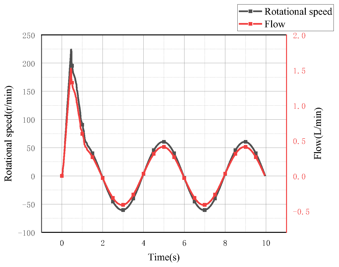
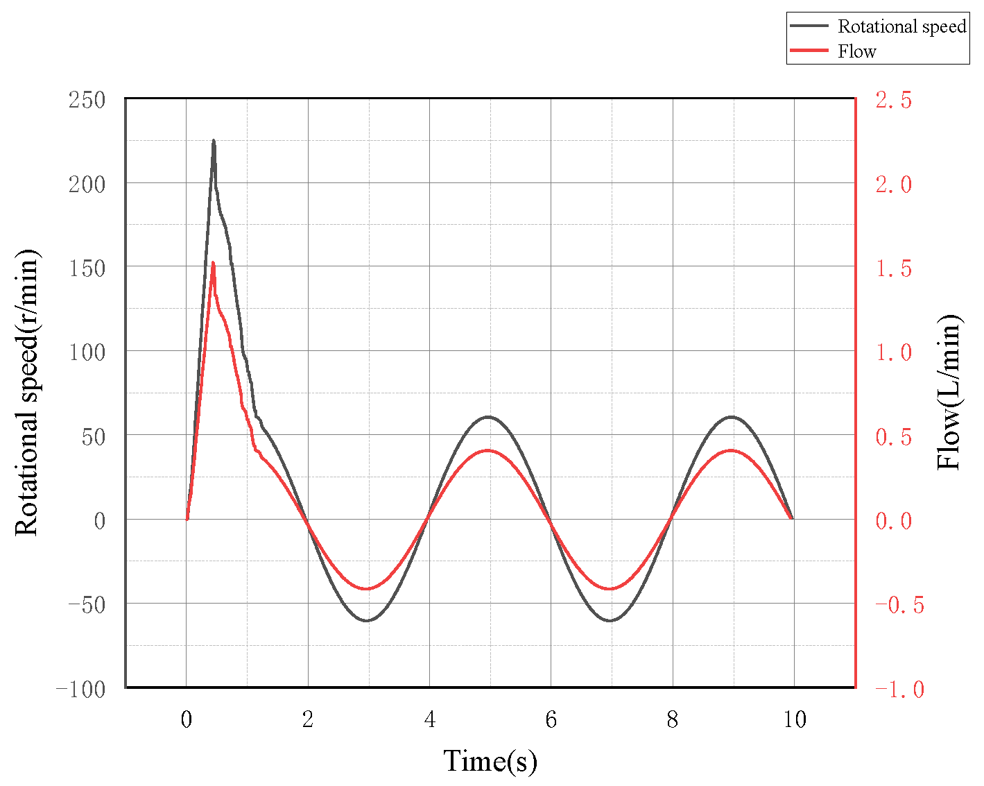
5.2.4. System Speed and Flow Analysis

When using the observer–sliding mode control method, the speed of the servo motor and the process of system flow and pressure changes are observed, as shown in Figure 19. The servo motor speed rises rapidly to 224 r/min approximately during the start-up process, and the flow rate is 1.6 L/min. After that, the flow rate is stabilized at ±60 r/min approximately, and the flow rate is also stabilized at ±0.5 L/min. The system flow rate can respond quickly and fluctuate less with the change in speed. The dynamic response speed of the PID control and sliding mode control methods can be improved significantly.

Figure 19. Speed-flow variation curve under variable load conditions.

5.3. Test Validation Results

5.3.1. Test Validation of PID Parameter Optimization in Constant Target Tillage Depth Values

In this paper, the proposed PID control optimization will be experimentally verified by using a semi-physical testbed, which is built to change and optimize the PID control parameters in constant target with all other conditions being equal. It verifies a better improvement over conventional PID control with the simulation results presented above.

As shown in Figure 20, after collecting and collating the experimental data, the system reached the displacement target value at 3.55 s without optimizing the PID control parameters. After parameter optimization, the system reached the displacement target value at 2.12 s, an improvement of 1.43 s over the response time of the PID control that is not optimized and a 40% improvement in response efficiency.

Figure 20. PID control in displacement mode compared with optimized PID control in constant target.

As shown in Figure 21, without optimization of the PID control parameters, the system pressure reaches the target pressure value at 2.43 s. After parameter optimization, the system has fluctuations with a peak value of 52.82 bar from 2.01 s to 2.1 s, and then quickly plateaus and finally reaches the target displacement value at 2.32 s, 0.11 s quicker than the response time of the not yet optimized PID control, which is an improvement of 4.5%.

Figure 21. PID control in pressure mode compared with optimized PID control in constant target.

After verification on a semi-physical testbed, the existence of an ideal state in the joint simulation led to deviations within a controlled range between the test data and the simulation data. After test verification and joint simulation, it was verified that the optimized PID control has a faster response and greater stability than the conventional PID.

5.3.2. Test Results for Constant Target Tillage Depth Values

The test equipment is used to verify the displacement and pressure control effects of the system with different control strategies for a fixed tillage depth value.

Using the test equipment to verify the control strategy of the simulation, the step displacement signal of the hydraulic cylinder in 0–0.5 m was collected through the displacement sensor, as shown in Figure 22. The response speed of the PID control in the test verification was 2 s, which was 0.11 s slower than the 1.89 s in the simulation test due to the delay of the signal transmission, and 1 s slower than the response speed of the theoretical expectation curve of 1 s; the response speed of the sliding mode control response speed was 1.4 s, 0.08 s slower than the response time of 1.32 s in the simulation test using sliding mode control, but the sliding mode control in the experimental verification was about 5% larger than the sliding film jitter amplitude in the simulation test; in the experimental verification, the response speed of observer–sliding mode control was 1.30 s, 0.05 s slower than the response time of 1.25 s in the simulation test. However, after the test, it was verified that the jitter phenomenon of sliding mode control was still effectively solved by using observer–sliding mode control. Compared with other control strategies, the response is faster and more accurate.

Figure 22. Displacement response curve for fixed tillage depth values.

The system pressure was collected through the pressure sensor in the experimental equipment to verify the step signal response of the system from 0 to 50 bar with various control strategies, as shown in Figure 23. The system reached 50 bar at 1 s under theoretical control; when PID control was used, the pressure slowly increased from 0 s, but after 1.89 s, there was a fluctuation beyond the target value, and then at 2.12 s, the pressure quickly dropped to the target value and stabilized; with sliding film control, the system response time iwa 1.12 s and reached the target value after 1.12 s, but after 1.12 s, the system had a continuous jitter from 49.1 to 52.8 bar, causing the system to be unstable. For the continuous jitter problem in sliding mode control, the observer–sliding mode control strategy was used after testing. The response time of observer–sliding mode control was about 1.09 s, which was 42% faster than the response time of PID control and 2.1% faster than the response time of sliding mode control. At about 0.91 s, the system also had a fluctuation beyond the target value, which was similar to PID control, with a fluctuation value of 2 bar, and then decreased rapidly and reached the expected. After the target value is reached, the system stabilizes [28].

Figure 23. Pressure response curve for fixed tillage depth values.

After experimental verification, the values are in general agreement with the simulated values above, and the error value is below 5%, which fully verifies that the use of the observer–sliding mode control strategy is superior to PID control and sliding mode control.

When using the observer–sliding mode control, the flow curve of the servo motor and the system in the power unit was collected, as shown in Figure 18.

As shown in Figure 24, after using the observer–sliding mode control, the servo motor from the start of operation continued to rise in 0.45 s. The speed reached a maximum of 551 r/min (at this time, the system flow rate was 3.6 L/min). After the running speed was reduced, or after 1.15 s, the servo motor stopped (at this time, the system flow rate was 0 L/min). The system reached the step target value (the actual target plowing target position). Combined with the displacement and pressure curves above, the servomotor and flow rate trends are consistent with the displacement and pressure curves, verifying the correctness of the test.

Figure 24. Variation of servo motor speed and flow rate for fixed tillage depth values.

5.3.3. Test Validation of PID Parameter Optimization in Continuously Varying Target Tillage Depth Values

In this paper, the proposed PID control optimization will be experimentally verified by using a semi-physical testbed, which is built to change and optimize the PID control parameters in constant target with all other conditions being equal. It verifies a better improvement over conventional PID control with the simulation results presented above.

As shown in Figure 25, without optimizing the PID control parameters, the system runs for one cycle at 3.53 s and reaches the target peak at 1.47 s. After parameter optimization, the system runs for one cycle at 3.15 s and reaches the target peak at 1.18 s. After analysis, the one-cycle running time is improved by 0.38 s, and efficiency is increased by 10.7% compared to the PID control that is not optimized; the target peak time is improved by 0.29 s, and efficiency is increased by 19.7%.

Figure 25. PID control in displacement mode compared with optimized PID control varying target.

As shown in Figure 26, without optimizing the PID control parameters, the system runs for one cycle at 4.42 s and reaches the target peak at 1.45 s. After parameter optimization, the system runs for one cycle at 4.14 s and reaches the target peak at 1.19 s. After analysis, the one-cycle running time is improved by 0.28 s, and efficiency is increased by 6% compared to the PID control that is not optimized; the target peak time is improved by 0.26 s, and efficiency is increased by 17.9%.

Figure 26. PID control in pressure mode compared with optimized PID control in varying target.

5.3.4. Test Results for Continuously Varying Target Tillage Depth Values

The test equipment is used to verify the displacement and pressure control of the system with different control strategies for continuously varying tillage depth values.

In the case of continuously varying plowing depths, the controller collects the hydraulic cylinder sensor signal and records the continuous displacement change of the hydraulic cylinder piston rod under continuously varying plowing depths, as shown in Figure 27 [28].

Figure 27. Displacement response curve for continuously varying plough depth values.

As shown in Figure 27, the maximum tillage depth was set at 0.4 m, and the tractor was simulated to change continuously within the maximum tillage depth value; the PID control reached the maximum tillage depth at 1.12 s, 5.05 s, and 9.1 s under three tillage depth changes, and the response time was longer; the slide film control reached the maximum tillage depth at 0.72 s, 4.69 s, and 8.7 s under three tillage depth changes, and the response time was 35% lower than the PID control. Compared with the PID control, the response time was reduced by 35%. However, under the slide film control, there was a continuous jitter vibration with the amplitude of 0.042 m in the process of continuous change, which caused the instability of the system; for the jitter vibration problem of slide film, the design adopted the observer–slide film control, and the maximum tillage depth was reached at 0.71 s, 4.65 s, and 8.67 s under three tillage depth changes, respectively. Compared with the sliding film control, the response speed is not greatly improved, but it solves the continuous jitter vibration problem, which is closer to the theoretical response curve, and improves the stability of the system.

As shown in Figure 28, the controller collected the pressure sensor information to detect the variability of the system pressure under different tillage depth values to verify the degree of system pressure response under different control strategies. They are 0.7 s, 4.6 s, and 8.5 s, respectively. In addition, the response efficiency was increased by 36.4% compared with the PID control. However, the system pressure response curve under the sliding mode control also generated the phenomenon of jitter vibration with an amplitude of 6 bar, and the existence of this phenomenon caused the instability of the system; to address this problem, the observer–sliding mode control was adopted to suppress the jitter vibration phenomenon appearing in the sliding film control, and, under the observer–sliding mode control, the system pressure reached the maximum pressure at 0.65 s, 4.65 s, and 8.45 s, respectively, which is the closest to the ideal state curve and can improve the jitter phenomenon, thus improving the response and stability of the system.

Figure 28. Pressure response curve for continuously varying tillage depth values.

When using the observer–sliding mode control, the flow curve of the servo motor and the system in the power unit was collected, as shown in Figure 21.

As shown in Figure 29, after using the observer–sliding mode control, the servomotor continuously rose from the start of operation, and reached a maximum speed of 225 r/min in 0.65 s (the system flow rate is 1.52 L/min at this time), and the speed-flow rate continued to decrease after operation. At 2 s, the servo motor stopped running (the system flow rate was 0 L/min at this time), and after starting from 2 s with a cycle of 4 s, the motor reversed in the 2–4 s time period. The system flow gradually increased sinusoidally. In 4 s, the motor switched running direction, and so on, so that the tractor could continuously switch the tillage depth target value of the action process. Combined with the above displacement and pressure curves, the servo motor and flow trends are consistent with the displacement and pressure curves, verifying the correctness of the test.

Figure 29. Variation of servo motor speed and flow rate for continuously varying tillage depth values.

6. Conclusions

To address the problem of jitter and vibration in the single sliding mode control in the tractor electro-hydraulic lifting system, an observer–sliding mode control strategy was designed, which was reasonable and could achieve a faster response and more accurate position control of the hydraulic cylinder in the system.

This study establishes a joint simulation model of MATLAB/Simulink and AMESim to verify that the observer–sliding mode controller is effective in improving the control accuracy of the tractor electro-hydraulic lifting system, which can give full play to the characteristics of the two software programs and help to analyze the system performance.

The observer–sliding mode control strategy was applied to the control of the tractor electro-hydraulic lifting system, which greatly improved the response frequency of the system, ensured the stiffness and robustness of the system, and proved to be an effective control method after simulation.

The electro-hydraulic lifting system uses a simple PID controller, which can basically achieve the following between command and feedback, verifying the rationality and correctness of the simulation model established. However, it is difficult for the PID controller to meet the control requirements of the electro-hydraulic servo pump control system for high precision and high response. Therefore, the proposed observer–sliding mode control strategy can better improve the system control performance in terms of system non-linear disturbance, following error abatement and external anti-interference performance.

At present, the application of electro-hydraulic lifting system energy saving is still a major problem. In the electro-hydraulic lifting system, a closed pump control system is used, which can eliminate the overflow loss and reduce energy loss. At the same time, for the two problems of poor robustness and that the control accuracy of the pump control system is not high, it can be further improved by changing the control strategy to improve the control accuracy. So, pump control will become a future trend due to its irreplaceable superiority. In the future, it can be applied to heavy vehicle steering, vehicle lifting devices, and various engineering and special equipment.

In the electro-hydraulic lifting system, the durability and safety of hydraulic components are particularly important, and the intelligence of hydraulic components is directly reflected in the life of the product, which will also promote the reliability of hydraulic products research. Now, most of them are used for the protection after the accident, and, in the future, they can be applied to the online fault monitoring and diagnosis technology to detect the early failure of the ageing hydraulic components, to improve the working period, and to ensure the life of the system. In the future, the pump can even be installed directly with the servo motor without piping.

For the electro-hydraulic lifting system, control precision is not high; in addition to a changing control strategy, the use of a high-performance servo motor with various types of sensors and other measures can also be considered in the future. Through the corresponding closed-loop control, a more precise rear axle steering control can be achieved. In the future, a dual-displacement design (large/small displacement) can be adopted: large displacement is used for fast movement and small displacement for precision control.

References

- Li, L.S. Discussion on the Development of Advanced Technology of Tractors in China. Agric. Technol. Equip. 2021, 10, 55–57. [Google Scholar]
- Wang, Y.S.; Wei, G.J. Tractor electro-hydraulic suspension technology application status and outlook. Jiangsu Agricultural Mechanization. Jiangsu Agric. Mech. 2022, 01, 36–37. [Google Scholar]
- Kut’kov, G.M. The development of the technical concept of the tractor. Tract. Agric. Mach. 2019, 86, 27–35. [Google Scholar] [CrossRef]
- Volk, R.; Rambhia, M.; Schultmann, F. Urban Resource Assessment, Management, and Planning Tools for Land, Ecosystems, Urban Climate, Water, and Materials—A Review. Sustainability 2022, 14, 7203. [Google Scholar] [CrossRef]
- Ou, Y.; Cui, T.; Lin, L. Development status and countermeasures of intelligent agricultural machinery equipment industry. Sci. Technol. Rev. 2022, 11, 55–66. [Google Scholar]
- Sun, X.X.; Lu, Z.X.; Song, Y.; Cheng, Z.; Jiang, C.; Qian, J.; Lu, Y. Development Status and Research Progress of a Tractor Electro-Hydraulic Hitch System. Agriculture 2022, 12, 1547. [Google Scholar] [CrossRef]
- Wang, L.; Wang, Y.; Dai, D.; Wang, X.; Wang, S. Review of electro-hydraulic hitch system control method of automated tractors. Int. J. Agric. Biol. Eng. 2021, 14, 1–11. [Google Scholar] [CrossRef]
- Singha, P.S.; Kumar, A.; Sarkar, S.; Baishya, S.; Kumar, P. Development of Electro-Hydraulic Hitch Control System through Lower Link Draft Sensing of a Tractor. J. Sci. Ind. Res. 2022, 81, 384–392. [Google Scholar]
- Pranav, P.K.; Tewari, V.K.; Pandey, K.P.; Jha, K. Automatic wheel slip control system in field operations for 2WD tractors. Comput. Electron. Agric. 2012, 84, 1–6. [Google Scholar] [CrossRef]
- Anche, G.; Velmurugan, M.; Kumar, A.; Subramanian, S.C.; Sreenivasulu, R.M. Model Based Compensator Design for Pitch Plane Stability of a Farm Tractor with Implement. IFAC-Pap. OnLine 2018, 51, 208–213. [Google Scholar] [CrossRef]
- Fernandez, B.; Herrera, P.J.; Cerrada, J.A. Self-tuning regulator for a tractor with varying speed and hitch forces. Comput. Electron. Agric. 2018, 145, 282–288. [Google Scholar] [CrossRef]
- Yang, J.R.; Li, N.; Li, R.C.; Jing, B.Y.; Li, H.; Mu, C.P. Control method and experimental study of tractor tillage depth based on sliding mode variable structure. Res. Agric. Mech. 2022, 44, 238–243. [Google Scholar]
- Li, M.S.; Ye, J.; Song, H.L.; Chen, J.J. Design and test of semi-physical simulation system for tractor electro-hydraulic suspension. J. Southwest Univ. Nat. Sci. Ed. 2018, 40, 14–21. [Google Scholar]
- Li, S.Z.; Wei, J.H.; Guo, K.; Zhu, W.-L. Nonlinear Robust Prediction Control of Hybrid Active-Passive Heave Compensator with Extended Disturbance Observer. IEEE Trans. Ind. Electron. 2017, 64, 6684–6694. [Google Scholar] [CrossRef]
- Zhang, W.; Liu, M.N.; Xu, L.Y. Design and simulation of hydraulic suspension system of electric tractor. Res. Agric. Mech. 2022, 44, 238–243. [Google Scholar]
- Xu, J.K.; Li, R.C.; Li, Y.C.; Zhang, Y.; Sun, H.; Ding, X.; Ma, Y. Research on Variable-Universe Fuzzy Control Technology of an Electro-Hydraulic Hitch System. Processes 2020, 9, 1920. [Google Scholar] [CrossRef]
- Gao, Q.; Lu, Z.X.; Xue, J.L.; Gao, H.; Sar, D. Fuzzy-PID controller with variable universe for tillage depth control on tractor-implement. J. Comput. Methods Sci. Eng. 2021, 21, 19–29. [Google Scholar] [CrossRef]
- Shafaei, S.M.; Loghavi, M.; Kamgar, S. A practical effort to equip tractor-implement with fuzzy depth and draft control system. Eng. Agric. Environ. Food 2019, 12, 191–203. [Google Scholar] [CrossRef]
- Timene, A.; Ngasop, N.; Djalo, H. Tractor-Implement Tillage Depth Control Using Adaptive Neuro-Fuzzy Inference System (ANFIS). Proc. Eng. Technol. Innov. 2021, 19, 53–61. [Google Scholar] [CrossRef]
- Zhou, M.K.; Xia, J.F.; Zhang, S.; Hu, M.; Liu, Z.; Liu, G.; Luo, C. Development of a Depth Control System Based on Variable-Gain Single-Neuron PID for Rotary Burying of Stubbles. Agriculture 2022, 12, 30. [Google Scholar] [CrossRef]
- Zhang, Z.; Xiao, Z.H.; Dai, L. Model order reduction method based on Laguerre polynomial expansion of matrix exponential function. Appl. Math. 2020, 33, 1002–1009. [Google Scholar]
- Liu, X.X.; Wang, Z.S. Lyapunov function optimization: Orthogonal matrix construction scheme. Control Theory Appl. 2022, 39, 1–10. [Google Scholar]
- Guo, X.P.; Wang, C.W.; Liu, H.; Zhang, Z.Y.; Ji, X.H.; Zhao, B. Extended-state-observer based sliding mode control for pump-controlled electro-hydraulic servo system. J. Beijing Univ. Aeronaut. Astronaut. 2020, 46, 1159–1168. [Google Scholar]
- Besova, M.; Kachalov, V. Analytical Aspects of the Theory of Tikhonov Systems. Mathematics 2021, 10, 72. [Google Scholar] [CrossRef]
- Zhang, S.Z.; Li, S.; Dai, F.Q. Integral Sliding Mode Backstepping Control of an Asymmetric Electro-Hydrostatic Actuator Based on Extended State Observer. Proceedings 2020, 64, 13. [Google Scholar]
- Hu, S.N.; Liu, J.H.; Qin, Z.T. The Number of Solutions of Certain Equations over Finite Fields. Wuhan Univ. J. Nat. Sci. 2022, 27, 49–52. [Google Scholar] [CrossRef]
- Cheng, C.; Liu, S.Y.; Wu, H.Z. Sliding mode observer-based fractional-order proportional–integral–derivative sliding mode control for electro-hydraulic servo systems. Proc. Inst. Mech. Eng. Part C J. Mech. Eng. Sci. 2022, 234, 1887–1898. [Google Scholar] [CrossRef]
- Du, H.; Shi, J.J.; Chen, J.D.; Zhang, Z.; Feng, X. High-gain observer-based integral sliding mode tracking control for heavy vehicle electro-hydraulic servo steering systems. Mechatronics 2021, 74, 49–52. [Google Scholar] [CrossRef]
Disclaimer/Publisher’s Note: The statements, opinions and data contained in all publications are solely those of the individual author(s) and contributor(s) and not of MDPI and/or the editor(s). MDPI and/or the editor(s) disclaim responsibility for any injury to people or property resulting from any ideas, methods, instructions or products referred to in the content. |
© 2023 by the authors. Licensee MDPI, Basel, Switzerland. This article is an open access article distributed under the terms and conditions of the Creative Commons Attribution (CC BY) license (https://creativecommons.org/licenses/by/4.0/).