An Improved Model Combining Outlook Attention and Graph Embedding for Traffic Forecasting

Abstract

Due to the highly non-linear nature of traffic data and the complex structure of road networks, traffic forecasting faces significant challenges. In this paper, we propose an improved model that combines outlook attention and graph embedding (MOAGE) for traffic forecasting, focusing on the construction of reasonable and effective spatio-temporal dependencies. Inspired by the idea of symmetry, MOAGE adopts a symmetrical encoder and decoder structure. Outlook attention blocks are important components of the encoder and decoder, consisting of spatial outlook attention and temporal outlook attention, used to model spatio-temporal dependencies in the road network. Cross attention are added to the model to reduce propagation errors. In addition, we learned the vertex representation of the graph via the node2vec algorithm and integrated the graph information into our model for a better prediction performance. Extensive experiments on two real datasets further demonstrate that the RMSE errors of the MOAGE on PEMS_BAY and METR_LA are reduced by approximately 14.6% and 12.2% for 60 min compared with the latest baseline models. Finally, the methodology used in this study will provide guidance to relevant ministries to better allocate transport resources and improve the efficiency and safety of traffic operations.

1. Introduction

In recent years, many countries have devoted themselves to intelligent transportation systems (ITSs). Advanced ITSs are inseparable from the processing of basic traffic data. At present, there are various data collection and processing methods in the transportation field, which can provide ITSs with multi-dimensional traffic data. Traffic forecasting, as an indispensable part of an intelligent transportation system, has attracted more and more researchers’ attention [1]. Accurate, real-time traffic forecasting is desired for relevant departments so as to better control traffic and reduce traffic congestion [2]. Unfortunately, traffic forecasting tasks face significant challenges owing to complex spatial–temporal correlations:

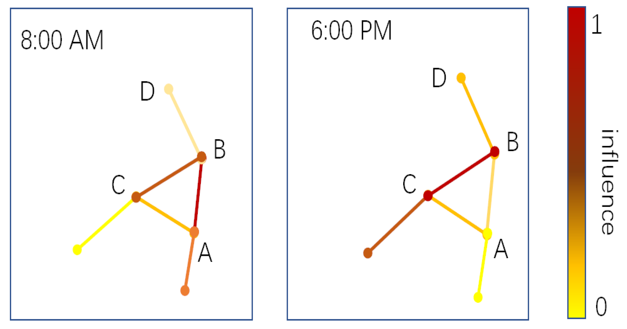
• Dynamic spatial correlations. Spatial dependencies between locations do not rely solely on the similarity of passed traffic flows. The traffic states between adjacent road segments in a road network are usually considered to interact with each other, and this impact is dynamic [3]. For example, as shown in Figure 1, for point A on a certain traffic segment, the influence of point B on its adjacent road segment on point A is different in the morning (8:00 a.m.) than in the evening (6:00 p.m.).
• Non-linear temporal correlations. For example, also for point A, its traffic status is not only affected by point B, but also closely related to its previous traffic status (traffic accidents, etc.). In other words, the current and future traffic state is affected by the historical traffic state.

Given the complex spatial–temporal dependencies of the traffic forecasting tasks, researchers in this field suggest many effective schemes. In the past few decades, mathematical statistical models have been widely used in the field of traffic forecasting. Generally speaking, such models [4] use historical data to make predictions, and assume that the predicted data and historical data have the same characteristics. These models [5] are simple in method, poor in accuracy, and are mostly static predictions, which cannot solve sudden traffic situations. Deep learning as a new machine learning approach has attracted extensive attention from researchers. It is a multi-layer perception containing multiple hidden layers, which realizes complex calculations by learning a deep nonlinear network structure. Thus, it can better restore the state of the traffic system and further achieve the purpose of predicting traffic flow more accurately [6]. Early recurrent neural network (RNN)-based models can establish connections for traffic data at adjacent moments and store memory through various gating mechanisms to learn the long-term dependencies of traffic flow sequences, showing strong advantages and potential in traffic flow prediction problems. However, these models cannot simulate the spatial structure of the traffic network in the real world. Convolutional neural networks (CNNs) [7,8,9] can further capture the characteristics of Euclidean space, which is not suitable for graph structure, so they are not the best way to learn the road network structure. It can be seen that the early algorithms have limitations. Recently, the convincing performance and high interpretability of graph neural networks (GNNs) make them a widely used method for graph structure analysis. Extending graph convolution operations to graph-structured data can capture traffic network information to model traffic forecasting problems [10,11,12]. In addition, the rapid development of technology has brought a new upgrade to intelligent transportation, but it has also brought a huge amount of traffic data. Traditional methods cannot solve such a huge amount of data at all, and traffic big data prediction through deep learning has become an inevitable trend.

In order to tackle the the traffic forecasting problem as reasonably and effectively as possible, we built an improved model combining outlook attention and graph embedding (MOAGE) that exploits an outlook-attention mechanism to efficiently encode fine-level information of both spatial and temporal dimensions. Furthermore, it simplifies the calculation process of attention weight through a reshape operation. In addition, we learned the vertex representation of the graph via the node2vec algorithm and integrated the graph information into our model for a better prediction performance. For the purpose of showing the traffic forecasting performance, we took the traffic speed prediction as an example. Nevertheless, our model is able to predict other traffic features efficiently.

In short, our main contributions are as follows:

• A spatial and temporal attention mechanism built on the outlook-attention is proposed to model complex spatial–temporal correlations. Moreover, we propose a gating mechanism to further fuse representations in both temporal and spatial dimensions.
• A cross attention mechanism is proposed to generate future traffic features by matrix multiplication of the traffic features outputted by the encoder with the corresponding attention weights, which further reduces the error propagation caused by different time steps.
• Extensive experiments were performed on two real-world large-scale highway datasets. Compared with the latest baseline models, for predictions 60 min ahead on PEMS_BAY and METR_LA, the RMSE errors of our model are reduced by approximately 14.6% and 12.2% at most, demonstrating the superior prediction performances of our model.

The rest of the paper is arranged as follows: Section 2 summaries previous work and limitations in this area. In Section 3, we describe the traffic forecasting problem in detail. In Section 4 and Section 5, we introduce our model in detail and analyze the experimental results, and finally conclude the paper and give out the future work.

2. Related Work

In an ITS, using the existing traffic data to accurately predict the future traffic situation in real-time is crucial for the control of traffic. Traffic flow forecasting has evolved through different stages.

Based on the statistical theory, the auto-regressive integrated moving average (ARIMA) [13,14] model is a rather rough forecasting approach that can only capture linear relationships. Therefore, the accuracy for the traffic forecasting task is not satisfactory. The Kalman filter cannot effectively deal with the randomness and complexity of traffic forecasting. Stephanedes applied the history average (HA) model [15] to urban traffic control in 1981. However, the HA model belongs to static prediction, which cannot reflect the uncertainty and nonlinear characteristics of dynamic traffic.

Machine learning models [16,17,18,19] such as the k-nearest neighbor algorithm (KNN) [20], which finds the nearest neighbors of the current real-time observation data from historical data and uses the prediction algorithm to obtain the traffic forecast at the next moment, have also been used.The core idea of the support vector regression (SVR) model [21] is to select the kernel function and train the support vector machine (SVM) to achieve the purpose of predicting the traffic flow.

Thanks to fast and cheap computing power and powerful hardware equipment, approaches based on deep learning have become the main method, and can characterize traffic features without requiring any prior knowledge. As a result, many deep learning approaches [11,22,23,24] are applied to the traffic forecasting task. For example, convolution long short-term memory (ConvLSTM), the study in [25] first proposed the combination of a convolutional neural network (CNN) and long short-term memory (LSTM) [26,27] to predict time-series problems.

However, conventional CNNs find it difficult to handle general network structures (transportation networks, etc.) [28]. In recent years, the abundance of graph data has led scholars to focus on building deep learning frameworks on graphs [29,30]. Benefiting from the excellent local feature extraction capability of the CNN and the natural dependencies between the nodes on the graph, the graph convolutional network (GCN) [31] has gradually become the most prominent and critical piece. However, most GCNs are not suitable for large-scale networks because of the extremely high computational complexity of the eigenvectors of the graph Laplacian matrix. For the spatial method, it relies on a large number of neighbor nodes when computing the representation of a new node, which also makes the calculation cost too high.

Recently, attention mechanisms [32,33] can be seen in diverse fields of deep learning, such as speech recognition, image classification, and natural language processing. The attention mechanism is essentially the same as the selective visual attention mechanism of humans. The core goal is to be able to select the more valuable part from the numerous information. Some researchers use the attention mechanism combined with graph convolution to predict traffic flow [7,31]. On the one hand, the limitation comes from the square-level computational complexity of self-attention, the memory bottleneck brought by stacking multiple layers, and the slow decoding prediction. On the other hand, the limitation is the high computational cost of graph convolution.

3. Problem Statement

In this paper, the weighted directed graph $G=(V,E,A)$ was used to denote the road network structure, where $\left|V\right|=N$ represents the set of vertices in the road network, E represents the set of edges, indicating the connectivity between vertices, and $A\in {\mathcal{R}}^{N\times N}$ represents the corresponding adjacency matrix. Each element $A_{v_i,v_j}$ represents the distance between vertex $v_i$ and $v_j$.

We used the graph signal $x_t\in {\mathcal{R}}^{N\times C}$ to represent the traffic situation at time step t, where C represents the number of traffic features. Information $\chi =(x_{t_1},x_{t_2,...x_{t_p}})$ for historical p time steps of a given traffic road accurately predicting the traffic conditions of the corresponding vertices in the next $\tau$ steps is our core goal, represented as $\chi =(x_{p+1},x_{p+2},...x_{p+\tau })$.

During the training fomentation, minimizing the error between the predicted value and the ground is our core idea: the smaller the error, the better the forecasting performance. ${\tilde{\mathcal{Y}}}_t$ and ${\widehat{\mathcal{Y}}}_t$ were used to represent the ground and the predicted value, respectively; thus, we formulated the loss function in the form:

$$\begin{array}{c}\hfill f\left(\alpha \right)=\frac{1}{\tau }\sum _{t=t_{(p+1)}}^{t_{(p+\tau )}}|{\tilde{\mathcal{Y}}}_t-{\widehat{\mathcal{Y}}}_t|\end{array}$$

(1)

where $\alpha$ means all trainable parameters.

In the next section, we illustrate our method in details. For ease of clarity, we list all symbols in this paper in

Table 1. Description of the main symbols in this paper.

Notation	Description
G	A graph.
V	Vertices of a graph, $\left|V\right|=N$.
p	Historical time step.
$\tau$	Future time step.
D	Dimensions of embedding.
K	The number of attention heads.
d	The dimension of each attention head.
$A,A_{v_i,v_j}$	Adjacency matrix of a graph and each of its elements.
$x_t\in {\mathcal{R}}^{N\times C}$	The traffic situation at time step t.

.

4. Methodology

4.1. Model Architecture

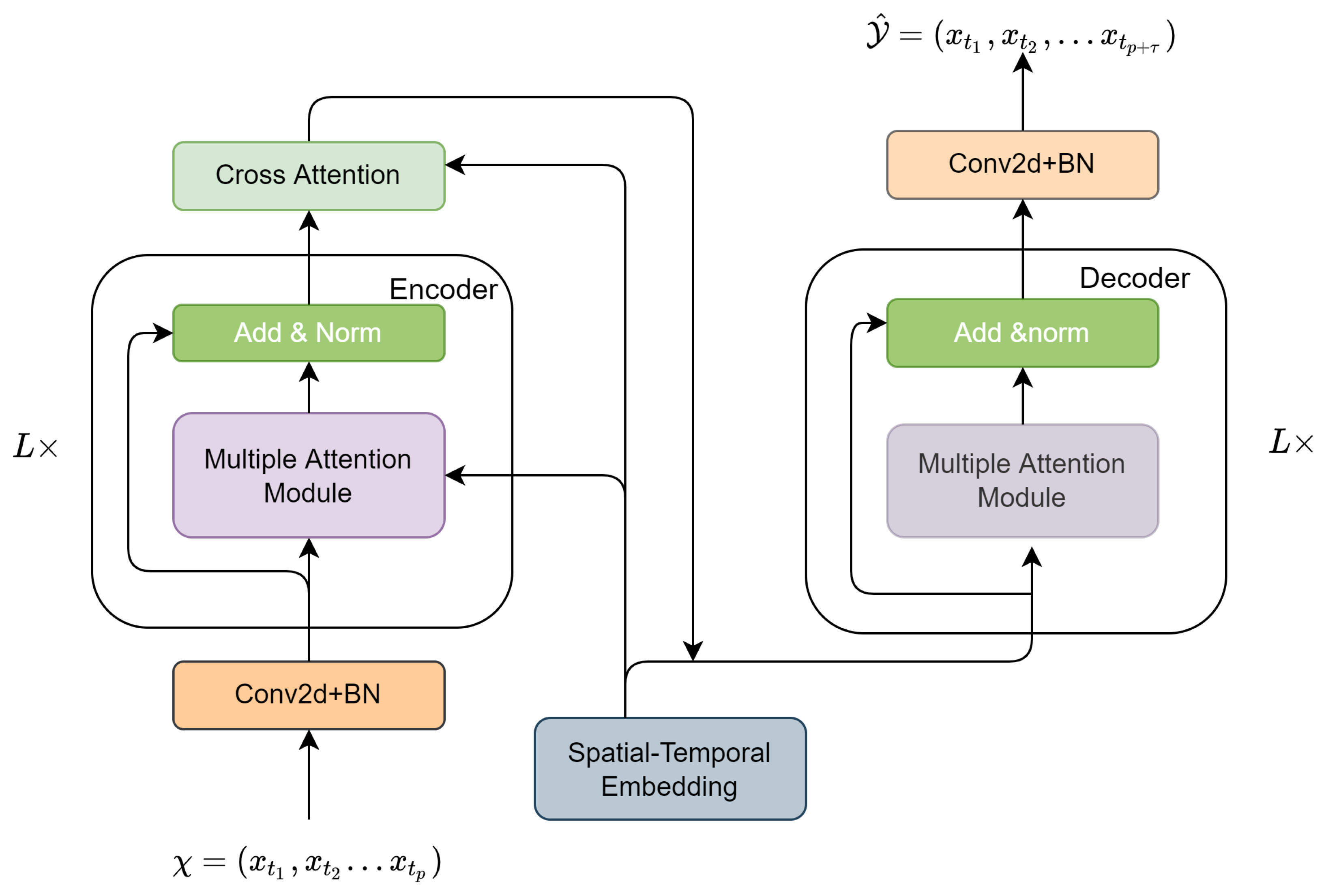
We will introduce the architecture of the improved model that combines outlook attention and graph embedding (MOAGE) to forecast traffic in the road network. MOAGE consists mainly of an encoder and a decoder, both of which are composed of outlook attention blocks. The outlook attention blocks contain spatial outlook attention and temporal attention via a gated mechanism. In addition, we have added cross attention between the encoder and decoder. The spatial and temporal embedding is added to better construct spatio-temporal dependencies.

As shown in Figure 2, our model adopts an encoder–decoder structure. The input historical data $\chi \in {\mathcal{R}}^{p\times N\times C}$ are mapped to $H^{\left(0\right)}\in {\mathcal{R}}^{p\times N\times D}$ through two fully connected layers before entering the encoder. After that, the output $H^{\left(l\right)}\in {\mathcal{R}}^{p\times N\times D}$ can be obtained from the input $H^{\left(0\right)}$ through an encoder composed of multiple attention modules. After the encoder, we added a cross attention layer to generate the future traffic feature $H^{(l+1)}\in {\mathcal{R}}^{\tau \times N\times D}$ as the input of the decoder. Next, the decoder corresponding to the encoder also stacks L attention modules and generates the output $H^{(2l+1)}\in {\mathcal{R}}^{\tau \times N\times D}$, and ultimately generates the predicted value $\widehat{\mathcal{Y}}\in {\mathcal{R}}^{\tau \times N\times C}$ through the fully connected layer.

In particular, either the encoder or the decoder contains L attention modules and residual connections [34]. The spatial attention component, the temporal attention component, and the gated mechanism together make up the multiple attention modules. Self-attention focuses on coarse global dependencies, whereas outlook-attention pays more attention to fine-level features, which is very beneficial for performance recognition. Therefore, we adopted the outlook-attention in both spatial and temporal dimensions. A cross attention component was also added to the model to reduce the propagation of errors.

Moreover, we embedded the graph structure through node2vec to obtain a graph vertex representation, and combined temporal information to obtain spatial–temporal embedding. The following is a detailed illustration of the model.

4.2. Spatial–Temporal Embedding

Owing to the complexity of the road network structure, the traffic conditions of different road segments are usually considered to be different. To obtain a better performance in traffic forecasting, it is crucial to integrate road information into the forecast pattern [35]. For keeping the complete invariance of the graph structure information as much as possible, we employed the node2vec [36] algorithm to obtain the vertex representation of the graph. node2vec can be seen as an extension of deepwalk, which combines depth-first search (DFS) or breadth-first search (BFS) random walks. node2vec controls whether the model prefers BFS or DFS by regulating the parameters of the direction. Furthermore, to integrate the input of the entire model into a unified form, these pre-trained vectors were sent to a fully connected layer for processing. Finally, we trained 1000 epochs to obtain spatial embedding, denoted as $e_{v_i}^S\in {\mathcal{R}}^D$, where $v_i\in V$. As the graph G has multiple vertices, we obtained the final spatial embedding $e^S\in {\mathcal{R}}^{N\times D}$, where N represents the numbers of V.

However, spatial embedding can only provide a static spatial representation, and cannot represent the dynamic relationship between complex road networks. Therefore, we propose temporal embedding to capture the dynamic characteristic: it encodes all time slices into a vector. Let us divide a day into t time slices; then, for each time slice, we performed one-hot encoding according to the seven days in the week and the specific time in each day, where the encoded vectors can be expressed as ${\mathcal{R}}^7,{\mathcal{R}}^T$, respectively. Then, they were concatenated with the vector form ${\mathcal{R}}^{T+7}$. Subsequently, we pre-processed them like spatial embedding to obtain a unified form. Thus, the temporal feature can always be represented as $e_{t_i}^T$, where $t_i\in t_1,t_2,...t_{p+\tau }$.

In order to obtain vertex representations at different time steps, we combined the above spatial and temporal embedding to obtain spatial–temporal embedding (STE). Therefore, for any time step $t_j$ and any vertex $v_i$, STE can be defined as $e_{v_i,t_j}=e_{v_i}^S+e_{t_j}^T$. Thus, the N vertices at $p+\tau$ time steps in STE can be represented as $E\in {\mathcal{R}}^{(p+\tau )\times N\times D}$.

In summary, STE contains the structure information of the graph and the time information of the input data, and will be applied in spatial attention, temporal attention, and cross attention.

4.3. Outlook Attention Blocks

A spatial and temporal attention and gated mechanism together make up each attention module. We used $H^{l-1}$ to represent the input of the lth module, and $H_S^l$ and $H_T^l$ to represent the output of spatial attention and temporal attention in the lth module, respectively. After the gated mechanism, we can obtain the output $H^l$ of the lth module.

4.3.1. Spatial Outlook Attention

At the same moment, the traffic conditions of different roads have different influences on the traffic conditions of a certain road, and these influences are highly dynamic and time-varying. To model this property, we propose spatial outlook-attention [37] to obtain the dynamic correlation among different sensors in a road network. Different from self-attention, which focuses on the global dependency model at coarse level, outlook-attention effectively encodes finer level features and context into tokens, which innovates the way for attention generation for token aggregation. In particular, it is a mechanism for inferring surrounding markers directly from anchor markers via an efficient linear projection, thus avoiding expensive dot product computations. In this paper, a token can be understood as the input traffic feature.

The spatial outlook-attention process can be divided into the following three steps:

• Given an input $X\in {\mathcal{R}}^{T\times N\times D}$, map it into a new feature V, where T represents time steps, N represents the number of vertices, and D means D-dimensions.
• Generate an attention map.
• Obtain weighted features.

For each spatial location $(i,j)$, we computed its similarity to all of its neighbors in a local window of size $k\times k$ centered at $(i,j)$. In addition, in order to better obtain the feature V, we also connected the hidden states of STE. Finally, given an input X, each D-dimensional vertex representation was mapped. We used two linear layers (with weights $W_A^S\in {\mathcal{R}}^{D\times k^4}$ and $W_V^S\in {\mathcal{R}}^{D\times D}$) to map to weights $A^S\in {\mathcal{R}}^{T\times N\times k^4}$ and values denoting $V^S\in {\mathcal{R}}^{T\times N\times D}$, respectively. If $V_{{▵}_{i,j}}^S\in {\mathcal{R}}^{D\times k^2}$ is used to represent all the values of the local window centered at $(i,j)$, then we have

$$\begin{array}{c}\hfill V_{{▵}_{i,j}}^S=V_{i+p-⌊\frac{k}{2}⌋,j+q-⌊\frac{k}{2}⌋}\end{array}$$

(2)

where $0\le p,q<k$. It should be noted that the weight at position $(i,j)$ will be directly used as the attention weight of the value aggregation, which will use the reshape operation to obtain ${\tilde{A}}_{i,j}^S\in {\mathcal{R}}^{k^2\times k^2}$, and then use the softmax function, so the value mapping process can be denoted by the following function:

$$\begin{array}{c}\hfill Y_{{▵}_{i,j}}^S=Matmul\left(softmax\left({\tilde{A}}_{i,j}^S\right),V_{{▵}_{i,j}}^S\right)\end{array}$$

(3)

After aggregating the projected value representations, the final output can then be represented by the addition of different weighted values from the same position of distinct local panes. The specific formula is as follows:

$$\begin{array}{c}\hfill {\tilde{Y}}_{{▵}_{i,j}}^S=\sum _{0\le m,n<k}{Y}_{{▵}_{i+m-⌊\frac{k}{2}⌋,j+n-⌊\frac{k}{2}⌋}}^S\end{array}$$

(4)

In particular, so as to guarantee that our model can pay attention to the information of different subspaces and thus is able to capture richer feature information, we expanded the spatial attention into a multi-head attention mechanism [38]. The implementation of the multi-head attention mechanism is simple. Assuming that the head number is set to M, here, we only need to perform the following processing:

• Change the dimension of $W_A^S$ to $D\times M\times k^4$, which is equivalent to $M{W}_A$, similar to grouping.
• Generate M weights $A_m^S\in {\mathcal{R}}^{T\times M\times k^4}$.
• Generate M value representations, denoted as $V_m^S\in {\mathcal{R}}^{T\times M\times D_M}$, where $D_M\times M=D$.

Then, for any data pair $(A_m^S,V_m^S)$, the spatial outlook-attention is calculated separately, and the final aggregation results form multi-head attention ones.

4.3.2. Temporal Outlook Attention

The traffic state of a certain position is not only influenced by the traffic conditions of the surrounding adjacent locations but is also closely related to its previous traffic state, and the influence of the same location on itself over time is also different. The relationship changes non-linearly over time. To model this property, we propose temporal outlook-attention. Likewise, we concatenated the hidden states of STE and simultaneously employed a multi-head attention mechanism. Finally, given an input $X\in {\mathcal{R}}^{N\times T\times D}$, two linear layers (with weights $W_A^T\in {\mathcal{R}}^{D\times k^4}$ and $W_V^T\in {\mathcal{R}}^{D\times D}$) were used to generate weights $A^T\in {\mathcal{R}}^{N\times T\times k^4}$ and values denoting $V^T\in {\mathcal{R}}^{N\times T\times D}$, respectively. After obtaining the attention weights, ${\tilde{A}}_{i,j}^T$ was obtained through the reshape operation, and then the softmax function was used. Thus, the value mapping process can be expressed as:

$$\begin{array}{c}\hfill Y_{{▵}_{i,j}}^T=Matmul\left(softmax\left({\tilde{A}}_{i,j}^T\right),V_{{▵}_{i,j}}^T\right)\end{array}$$

(5)

After that, we obtained the final output by summing the different weights at the same location from distinct panes, which is

$$\begin{array}{c}\hfill {\tilde{Y}}_{{▵}_{i,j}}^T=\sum _{0\le m,n<k}{Y}_{{▵}_{i+m-⌊\frac{k}{2}⌋,j+n-⌊\frac{k}{2}⌋}}^T\end{array}$$

(6)

More importantly, we used outlook-attention rather than self-attention. This is due to the fact that, on the one hand, outlook attention encodes information by measuring the similarity between token representations, which is more suitable for our prediction task. On the other hand, outlook attention is a simple and efficient method for generating attention weights, and is computationally efficient at $N{k}^2$, where k denotes the size of the sliding window.

4.3.3. Gated Mechanism

It can be seen from the above analysis that, at a certain time step, the traffic state of a certain road is related to the previous traffic state and the traffic state of other roads at the same time. To this end, a gated mechanism is proposed to automatically integrate representations in both spatial and temporal dimensions. For example, the output results in the lth module of spatial attention and temporal attention modules can be denoted by $H_S^l$ and $H_T^l$, respectively, where $H_S^l$ and $H_T^l$ both have ${\mathcal{R}}^{T\times N\times D}$ in the encoder or decoder. Then, $H_S^l$ and $H_T^l$ can be fused according to the following formula:

$$\begin{array}{c}\hfill H^l=\mu \odot H_S^l+(1-\mu )\odot H_T^l\end{array}$$

(7)

with

$$\begin{array}{c}\hfill \mu =\sigma (H_S^l{W}_{\mu ,1}+H_T^l{W}_{\mu ,2}+b_{\mu })\end{array}$$

(8)

where $W_{\mu ,1},W_{\mu ,2}\in {\mathcal{R}}^{D\times D}$ and $b_{\mu }\in {\mathcal{R}}^D$ are trainable parameters, ⊙ means the Hadamard product, and $\sigma$ represents the sigmoid activation.

4.4. Cross Attention

While the model is training, using the result of the previous prediction as the input of the next step will generate errors. In order to reduce the propagation of errors in different time steps and effectually accelerate the convergence of the model, we added cross attention [39] between the encoder and decoder. It calculates the weight through the correlation between the next time slice and the past time slice and obtains the attention score through the softmax function, and thus uses the encoder’s traffic feature and the attention score to perform matrix multiplication to generate the future traffic feature. The cross attention process can be presented by the following equation:

$$\begin{array}{cc}\hfill \widehat{\alpha }& =softmax\left(f_{cr,1}^l\left(ST{E}_{his}\right)·f_{cr,2}^l\left(ST{E}_{pred}\right)\right)\hfill \end{array}$$

(9)

$$\begin{array}{cc}\hfill H^l& =\widehat{\alpha }{f}_{cr,3}^l\left(X\right)\hfill \end{array}$$

(10)

where $f_{cr,1}^l,f_{cr,2}^l,f_{cr,3}^l$ represent three different nonlinear projections, respectively, and $ST{E}_{his}$, $ST{E}_{pred}$ represent the traffic features of the historical time step after spatial–temporal embedding and the traffic features of the corresponding future time steps.

5. Experiments

In this section, we validated the forecasting performance of the model and the latest baseline approaches on two real large-scale highway datasets. The same datasets were used in the latest work, such as Graph WaveNet, GMAN, DCRNN, etc.

• PEMS_BAY [40] is the traffic data in San Francisco Bay Area collected by the California Department of Transportation, with 325 sensors collecting 6 months of data (2017.1.1∼2017.6.30).
• METR_LA dataset [41] is the data collected by the Los Angeles Highway Detector, containing 207 sensors collecting data for 4 months (2012.3.1∼ 2012.6.30).

The sensor distribution and statistical information for both datasets are shown in Figure 3 and

Table 2. Statistics of datasets.

Dataset	Samples	Node	Sample Rate	Time Span
METR_LA	34,272	207	5 min	4 months
PEMS_BAY	52,116	307	5 min	6 months

, respectively.

The time interval of both datasets is 5 min, and the input data are processed by z-score normalization. We divided the entire dataset with a ratio of 0.7, 0.2, 0.1 for training, validation, and test set, respectively. In addition, for the purpose of constructing the road structure more reasonably, we regarded each traffic detector as a vertex so that the distance between the vertices could be calculated. We defined the corresponding adjacency matrix according to the following formula:

$$A_{i,j}=\left\{\begin{array}{cc}0,\hfill & if{e}^{\left(\frac{-d_{v_i,v_j}^2}{{\sigma }^2}\right)}<\xi \hfill \\ e^{\left(\frac{-d_{v_i,v_j}^2}{{\sigma }^2}\right)},\hfill & otherwise\hfill \end{array}\right.$$

(11)

where $d_{v_i,v_j}$ represents the distance from $v_i$ to $v_j$, $\sigma$ represents the standard deviation of the distance, and $\xi$ means the threshold.

The following three indicators were selected to judge the forecasting performance of MOAGE and baseline approaches.

• Mean absolute error (MAE):

  $$\begin{array}{c}\hfill MAE=\frac{1}{N}\sum _{i=1}^N|{\tilde{\mathcal{Y}}}_t-{\widehat{\mathcal{Y}}}_t|\end{array}$$

  (12)
• Root mean squared error (RMSE):

  $$\begin{array}{c}\hfill RMSE=\sqrt{\frac{1}{N}\sum _{i=1}^N{|{\tilde{\mathcal{Y}}}_t-{\widehat{\mathcal{Y}}}_t|}^2}\end{array}$$

  (13)
• Mean absolute percentage error (MAPE):

  $$\begin{array}{c}\hfill MAPE=\frac{1}{N}\sum _{i=1}^N\left|\frac{{\tilde{\mathcal{Y}}}_t-{\widehat{\mathcal{Y}}}_t}{{\tilde{\mathcal{Y}}}_t}\right|\end{array}$$

  (14)

5.1. Hyperparameters

Similar to the existing work, we forecasted the traffic conditions of the future 15 min $(\tau =3)$, 30 min $(\tau =6)$, and 60 min $(\tau =12)$ from the observation data of the past 15, 30, and 60 min (p = 3, 6, and 12). The Adam [42] optimizer with a learning rate of 0.001 was chosen for training our model. We defined three hyperparameters $L,K,d$ as the number of attention modules, the number of attention heads, and the dimension of each attention head in our model.

In order to fully exploit the performance of the model, we tried to increase the number of attention modules to better refine the traffic features. Figure 4 shows the change in prediction performance with different numbers of attention modules for 60 min on PEMS_BAY. Through experiments, we found that, as L increases to 5, the network depth basically tends to saturate. Finally, we obtained that, when $d=8,K=8,L=5$, the prediction result is the best.

5.2. Experimental Results

The following baseline approaches were used as comparisons with the performance of our model:

• ARIMA [13], which models non-stationary time series, and its essence is the combination of difference operations and the ARMA model.
• FC_LSTM [43], which adopts a seq-to-seq model, and the main components of the encoder and corresponding decoder are the lstm layers.
• STGCN [44], which performs graph convolution operations in space, and exploits a one-dimensional convolution TCN to convolve all vertices in time, where the two alternately form space–time modules.
• DCRNN [40], which is a holistic approach used to capture spatial–temporal correlations using diffuse convolution and seq-to-seq architecture frameworks with predetermined sampling.
• GraphWaveNet [45], which mainly includes two modules, namely the GCN and TCN. The two modules are integrated to obtain the dependencies of time and space.
• GMAN [46], which adopts an encoder–decoder structure, and uses the node2vec algorithm to learn the vertex representation of the graph.

MAE, RMSE, and MAPE are three common regression model evaluation metrics that reflect the actual error in the predicted values, and we calculated the results for each baseline model using Equations (12)–(14).

Table 3. Comparison of experimental results between MOAGE and other baseline approaches on two real datasets.

Data	Method	15 min			30 min			60 min
		MAE	RMSE	MAPE	MAE	RMSE	MAPE	MAE	RMSE	MAPE
PEMS_BAY	ARIMA	1.62	3.30	3.50%	2.33	4.76	5.40%	3.38	6.50	8.30%
	FC_LSTM	2.05	4.19	4.80%	2.20	4.55	5.20%	2.37	4.96	5.70%
	STGCN	1.36	2.96	2.90%	1.81	4.27	4.17%	2.49	5.69	5.79%
	DCRNN	1.38	2.95	2.90%	1.74	3.97	3.90%	2.07	4.74	4.90%
	Graph WaveNet	1.30	2.74	2.73%	1.63	3.70	3.67%	1.95	4.52	4.63%
	GMAN	1.34	2.82	2.81%	1.62	3.72	3.63%	1.86	4.32	4.31%
	Ours	1.30	2.50	2.83%	1.59	3.21	3.30%	1.85	3.69	4.30%
METR_LA	ARIMA	3.99	8.21	9.60%	5.15	10.	12.70%	6.90	13.23	17.40%
	FC_LSTM	3.44	6.30	9.60%	3.77	7.23	10.09%	4.37	8.69	14.00%
	STGCN	2.88	5.74	7.62%	3.47	7.24	9.57%	4.59	9.40	12.70%
	DCRNN	2.77	5.38	7.30%	3.15	6.45	8.80%	3.60	7.59	10.50%
	Graph WaveNet	2.69	5.15	6.90%	3.07	6.22	8.37%	3.53	7.37	10.01%
	GMAN	2.77	5.48	7.25%	3.07	6.34	8.35%	3.40	7.21	9.72%
	Ours	2.74	4.82	7.17%	3.03	6.20	8.17%	3.40	6.33	9.50%

shows the experimental consequences of all models at 15 min $(\tau =3)$, 30 min $(\tau =6)$, and 60 min $(\tau =12)$ on two different datasets.

By comparing and analyzing the experimental results in Table 3, the following conclusions can be drawn:

• For the time series problem, compared with the classical time series approach, the deep learning method performs better, which indicates that the deep network has a powerful nonlinear expression ability for the traffic forecasting problem.
• All approaches based on deep learning frameworks, except STGCN, outperform FC_LSTM on both datasets, regardless of whether the prediction interval is lare or small.
• Combining the results of the two datasets, it can be clearly seen that MOAGE basically obtains the best forecasting performance, which indicates the superior performance of our model. For example, for the 60 min traffic forecasting, the RMSE errors of the GMAN, Graph WaveNet, DCRNN, STGCN, and FC_LSTM are increased by approximately 12.2%, 14.1%, 16.6%, 32.7%, and 27.2% compared with MOAGE for METR_LA. As for PEMS_BAY, the RMSE errors are 14.6%, 18.4%, 22.2%, 35.1%, and 25.6%, respectively.

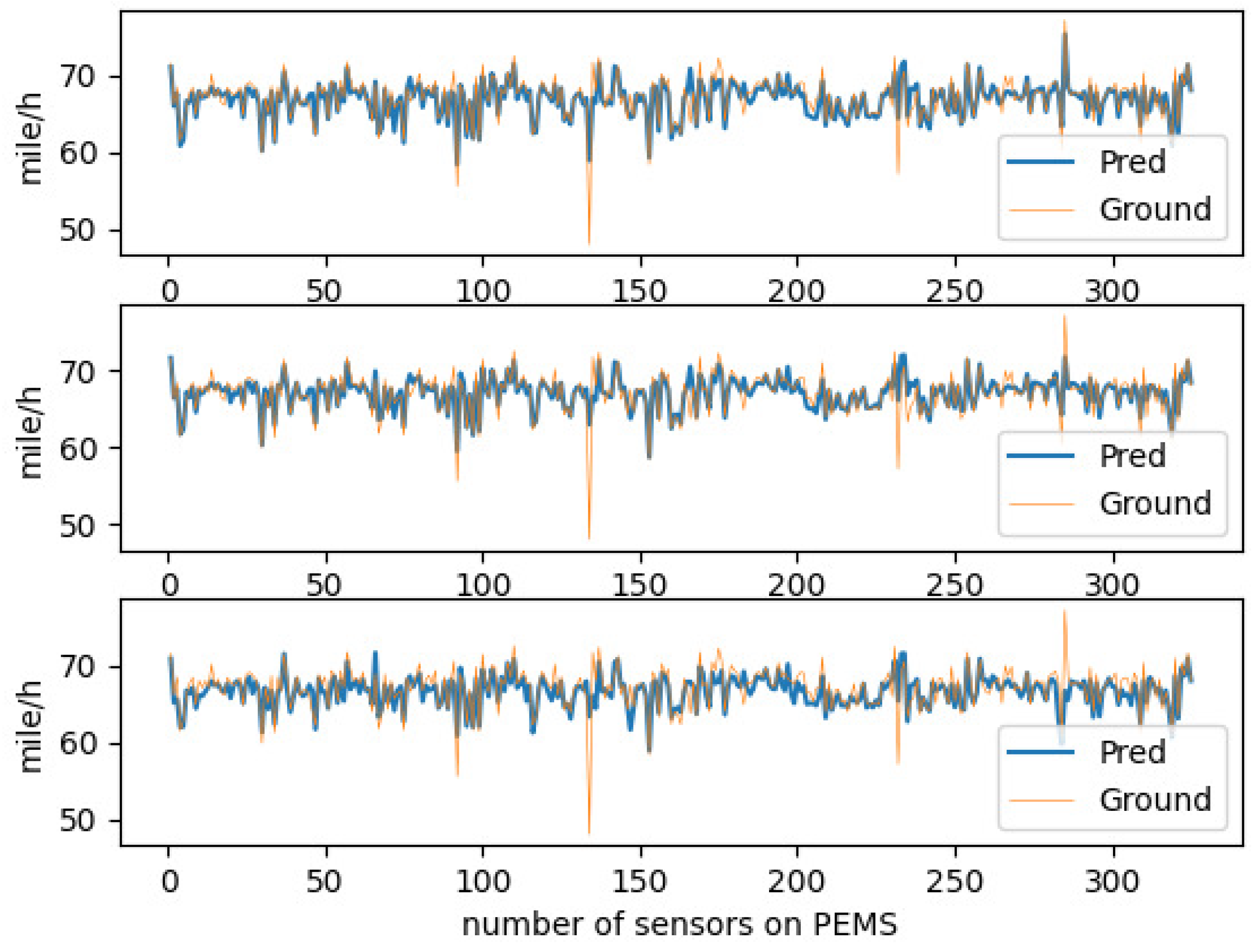
In order to perform a multifaceted and detailed study of the model, we chose to visualize the traffic speed prediction of the entire road network of PEMS_BAY at a certain moment. Figure 5 visualizes the change in the forecast performance curve as the forecast time interval becomes larger. By observing Figure 5, we can easily obtain the following information:

• The larger the prediction time interval, the worse the corresponding prediction performance gradually becomes.
• Overall, our model is still very accurate in capturing the change in the traffic speed trend. In particular, when the prediction interval is 15 min and 30 min, the RMSE of our model is 2.50 and 3.21, respectively, and the prediction performance is further improved compared to GMAN. As for the 60-min long-term forecast, the RMSE of our model is still reduced by approximately 0.63 compared to GMAN, which demonstrates the utility of our model in capturing dynamic spatial–temporal correlations in traffic forecasting.

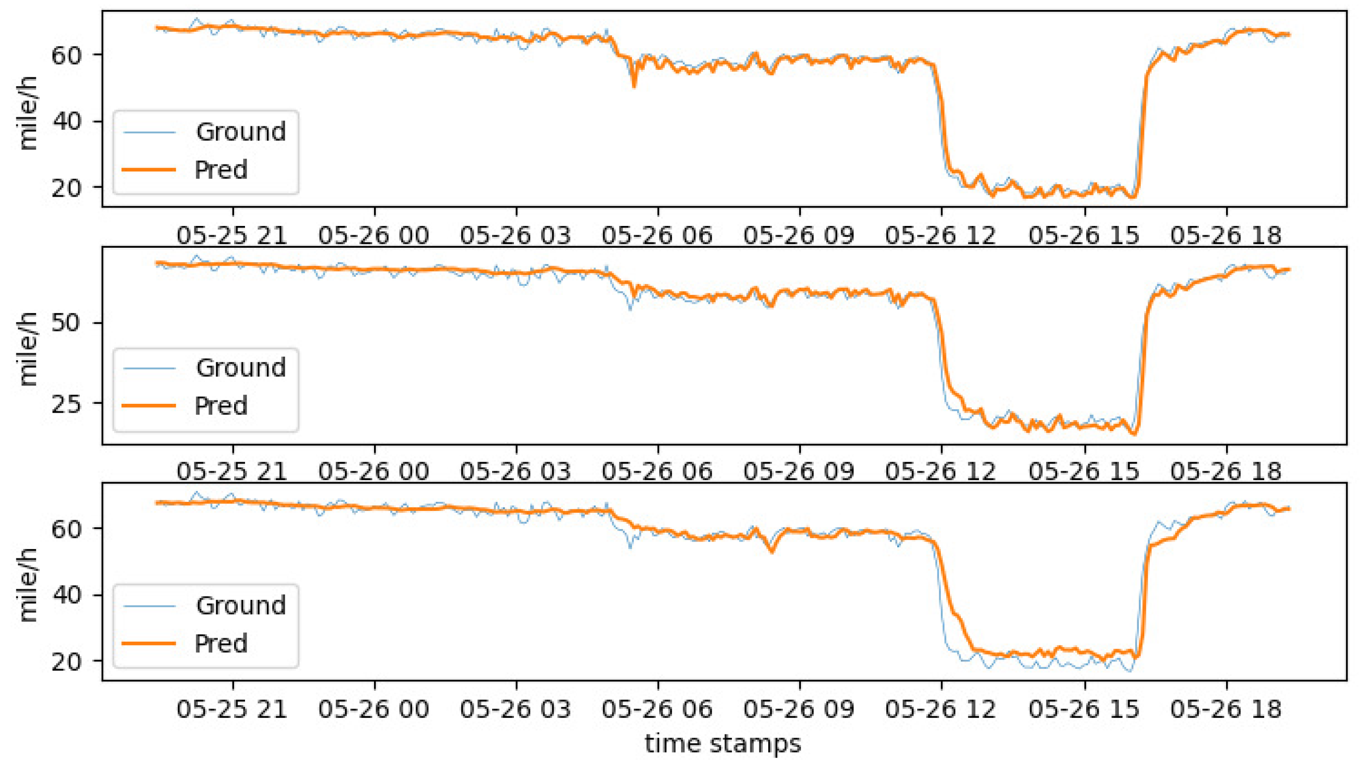
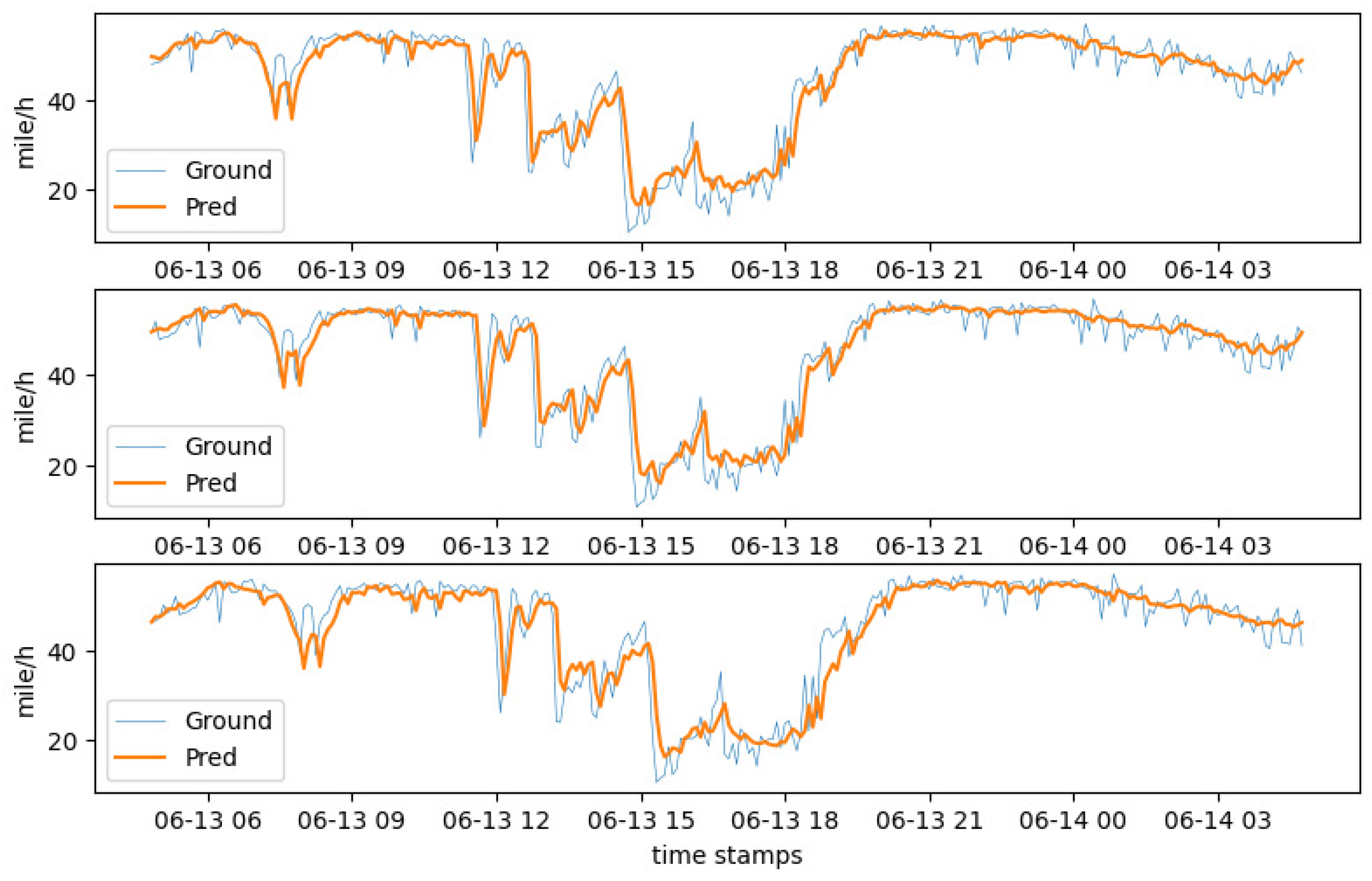
In addition, we also visualized the traffic speed on a given day on PEMS_BAY. Figure 6 shows the changes in forecasting property as the prediction interval increases.

Similarly, we also visualized the traffic speed of the METR_LA dataset on a certain day, and the visualization results are shown in Figure 7.

According to the analysis of the visualization results, for a prediction time of 15 min on PEMS_BAY, the RMSE error of MOAGE is reduced by 40.3% compared to FC_LSTM. When the prediction time increases to 30 min, the corresponding RMSE error is reduced by approximately 28.8%, and, for 60 min, it is reduced by approximately 25.6%. On the METR_LA, the RMSE of our model is also reduced to varying degrees relative to FC_LSTM, which indicates that MOAGE can obtain the first-rate forecasting property by continuous training, regardless of whether the prediction interval is small or large.

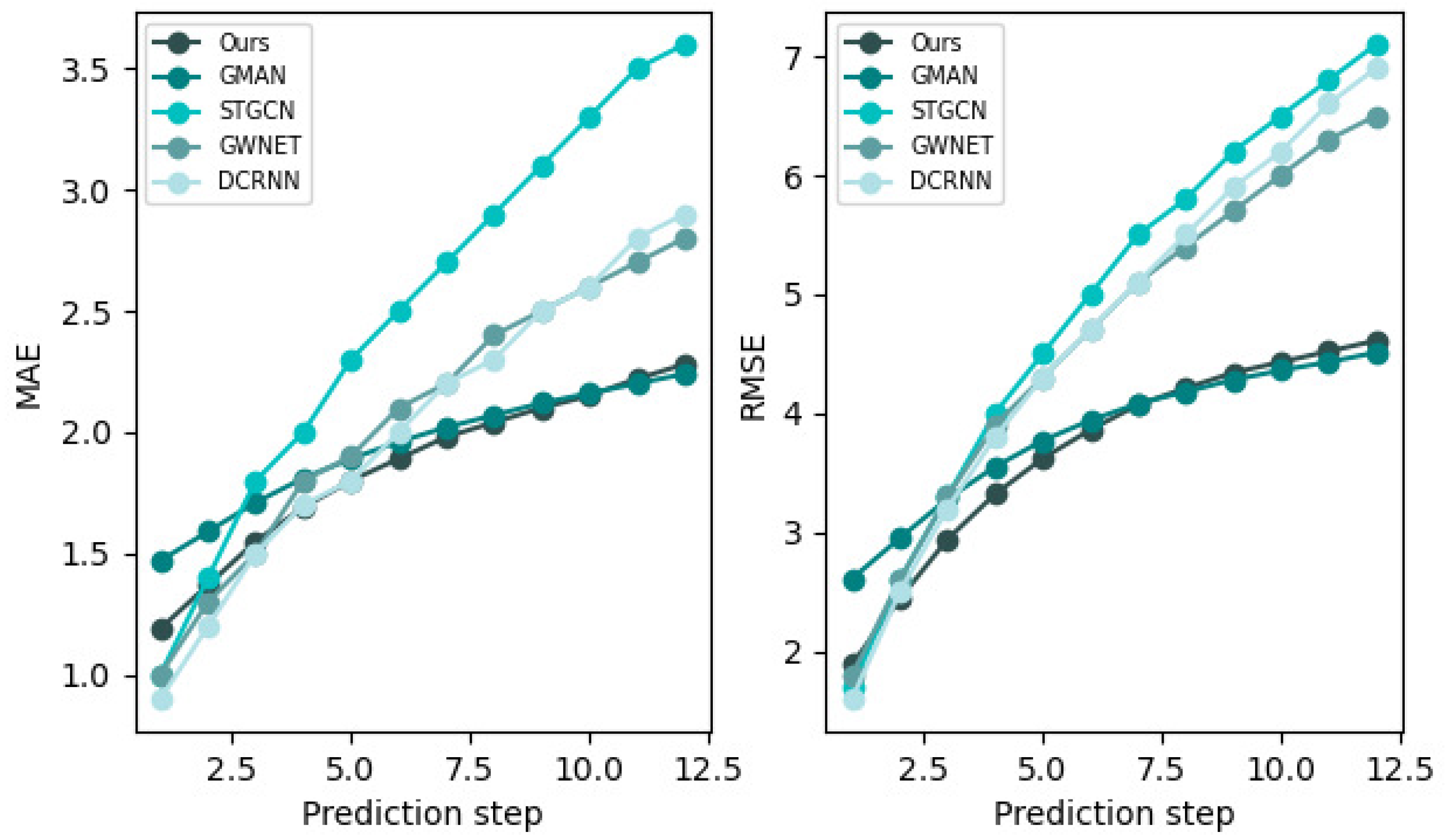
We also compared the experimental results of our model and baselines for the 60 min ahead prediction on the two datasets, and their performance changes are presented in the following Figure 8, Figure 9, Figure 10 and Figure 11, separately.

The results indicate that our model achieves the best results on the two datasets, which fully shows that our model is not only effective at short-term prediction, but also has an excellent performance in long-term prediction problems. We think this is because the model structure that we designed is better at capturing spatial dependencies at different time steps. Figure 10 and Figure 11 show the changes in the prediction performance of different approaches as the prediction interval gets larger. In conclusion, as the prediction time increases, the corresponding prediction difficulty also increases; hence, the prediction error also increases. Compared with FC_LSTM, DCRNN, and Graph WaveNet, etc., our model achieves the optimal effect, showing that the strategy of combining the attention mechanism and graph embedding is better.

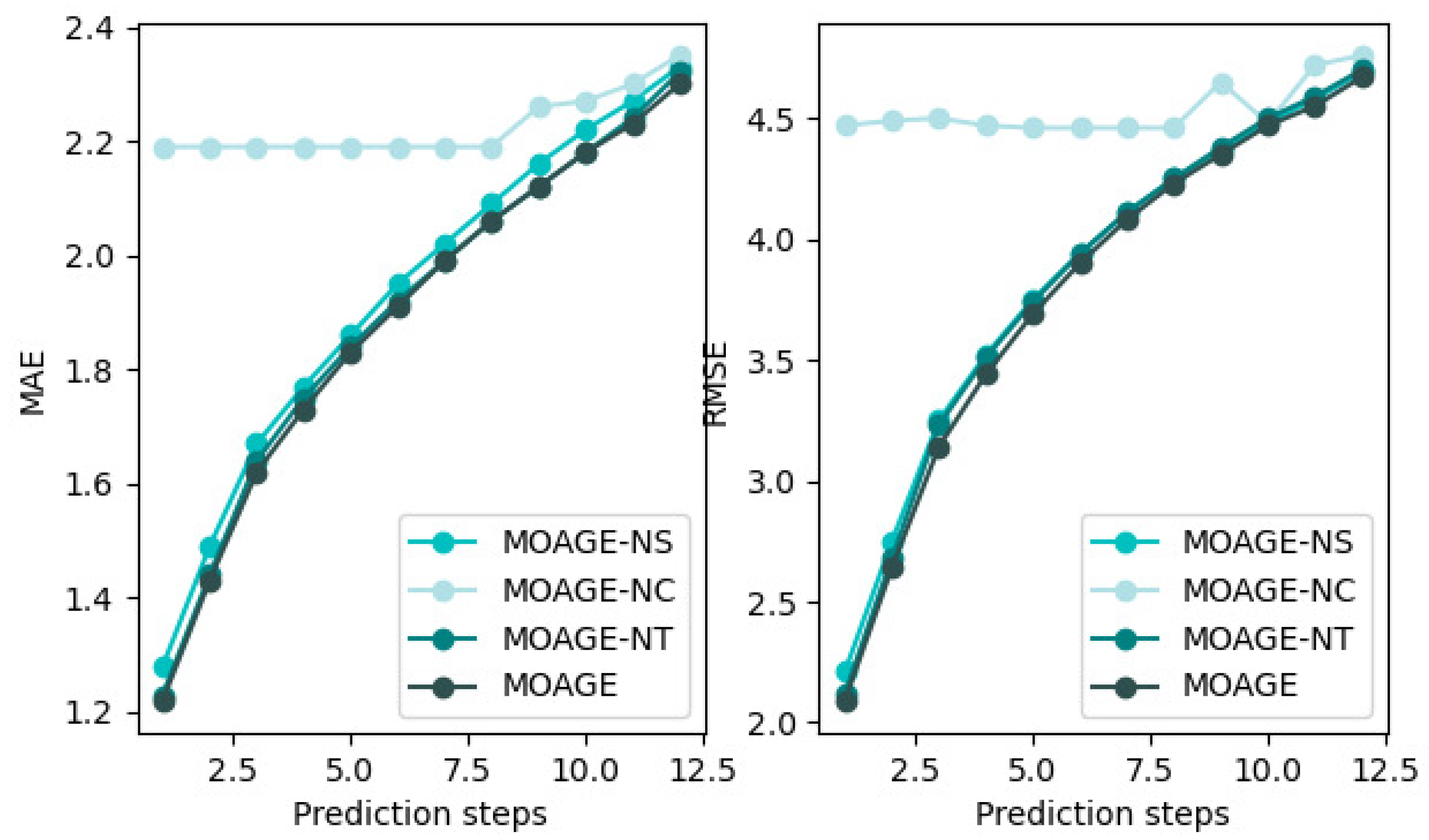
5.3. Validity of Each Component

To illustrate the validity of every component of the model, we took the prediction of 60 min traffic conditions as an example, and conducted ablation studies on the PEMS_BAY dataset. The spatial attention, temporal attention, and cross attention components of the model were removed, respectively. The remaining parts of MOAGE were called MOAGE-NS, MOAGE-NT, and MOAGE-NC, respectively. Figure 12 shows the metric of MAE and RMSE, from which, we can draw the following conclusions:

• When the prediction time interval is 60 min, the average RMSEs of MOAGE-NS, MOAGE-NT, MOAGE-NC, and MOAGE are 3.83, 3.81, 4.55, and 3.69, respectively. Moreover, it can be seen from the change in the curve that the prediction performance of MOAGE is always the best, which indicates that spatial attention and temporal attention are very effective in capturing complex spatial–temporal correlations.
• It can be found from the comparison in Figure 12 that MOAGE obtains better prediction results that of MOAGE-NC, which fully proves that cross attention has a relatively important position in reducing the propagation of deviations at different time steps and is an integral part of the framework.

6. Conclusions

In this paper, we propose a new deep learning framework, MOAGE, for predicting traffic conditions in road networks. Our model adopts an encoder–decoder architecture. Its stacked attention module has a powerful ability to capture long-term dependencies. In particular, we propose spatial outlook attention and temporal outlook attention with gated mechanisms to model complex spatio-temporal dependencies. We further propose cross attention to reduce the error propagation during the training process. Extensive experiments on two real datasets further demonstrate the excellent predictive performance of the model. However, there are still limitations to the model. For example, as the input time series becomes longer, the complexity of the model increases squarely. Therefore, it is our future work to alleviate this shortcoming; for example, by taking a pre-training approach to obtain rich hidden representations and using them for our prediction tasks. Moreover, our model can also be applied to other practical applications, such as rainfall forecasting.

References

- Zheng, C.; Fan, X.; Wen, C.; Chen, L.; Wang, C.; Li, J. DeepSTD: Mining spatio-temporal disturbances of multiple context factors for citywide traffic flow prediction. IEEE Trans. Intell. Transp. Syst. 2019, 21, 3744–3755. [Google Scholar] [CrossRef]
- Jian, Y.; Bingquan, F. Synthesis of short-term traffic flow forecasting research progress. Urban Transp. China 2012, 10, 73–79. [Google Scholar]
- Dong, C.J.; Shao, C.F.; Zhuge, C.X.; Meng, M. Spatial and temporal characteristics for congested traffic on urban expressway. J. Beijing Univ. Technol. 2012, 38, 1242–1246. [Google Scholar]
- Lin, G.; Lin, A.; Gu, D. Using support vector regression and K-nearest neighbors for short-term traffic flow prediction based on maximal information coefficient. Inf. Sci. 2022, 608, 517–531. [Google Scholar] [CrossRef]
- Shah, I.; Muhammad, I.; Ali, S.; Ahmed, S.; Almazah, M.; Al-Rezami, A. Forecasting Day-Ahead Traffic Flow Using Functional Time Series Approach. Mathematics 2022, 10, 4279. [Google Scholar] [CrossRef]
- Tao, Q.; Li, Z.; Xu, J.; Lin, S.; De Schutter, B.; Suykens, J.A. Short-term traffic flow prediction based on the efficient hinging hyperplanes neural network. IEEE Trans. Intell. Transp. Syst. 2022, 23, 15616–15628. [Google Scholar] [CrossRef]
- Guo, S.; Lin, Y.; Wan, H.; Li, X.; Cong, G. Learning dynamics and heterogeneity of spatial-temporal graph data for traffic forecasting. IEEE Trans. Knowl. Data Eng. 2021, 23, 5415–5428. [Google Scholar] [CrossRef]
- Ge, L.; Li, S.; Wang, Y.; Chang, F.; Wu, K. Global spatial-temporal graph convolutional network for urban traffic speed prediction. Appl. Sci. 2020, 10, 1509. [Google Scholar] [CrossRef]
- Li, M.; Zhu, Z. Spatial-temporal fusion graph neural networks for traffic flow forecasting. Proc. AAAI Conf. Artif. Intell. 2021, 35, 4189–4196. [Google Scholar] [CrossRef]
- Zhang, Y.; Lu, M.; Li, H. Urban traffic flow forecast based on FastGCRNN. J. Adv. Transp. 2020, 2020, 8859538. [Google Scholar] [CrossRef]
- Song, C.; Lin, Y.; Guo, S.; Wan, H. Spatial-temporal synchronous graph convolutional networks: A new framework for spatial-temporal network data forecasting. Proc. AAAI Conf. Artif. Intell. 2020, 34, 914–921. [Google Scholar] [CrossRef]
- Wu, Z.; Pan, S.; Long, G.; Jiang, J.; Chang, X.; Zhang, C. Connecting the dots: Multivariate time series forecasting with graph neural networks. In Proceedings of the 26th ACM SIGKDD International Conference on Knowledge Discovery & Data Mining, Virtual Event, 6–10 July 2020; pp. 753–763. [Google Scholar]
- Makridakis, S.; Hibon, M. ARMA models and the Box–Jenkins methodology. J. Forecast. 1997, 16, 147–163. [Google Scholar] [CrossRef]
- Ahmed, M.S.; Cook, A.R. Analysis of Freeway Traffic Time-Series Data by Using Box-Jenkins Techniques; Number 722; Transportation Research Record: Amsterdam, The Netherlands, 1979. [Google Scholar]
- Wei, G. A Summary of Traffic Flow Forecasting Methods. J. Highw. Transp. Res. Dev. 2004, 3, 82–85. [Google Scholar]
- Wu, C.H.; Ho, J.M.; Lee, D.T. Travel-time prediction with support vector regression. IEEE Trans. Intell. Transp. Syst. 2004, 5, 276–281. [Google Scholar] [CrossRef]
- Yao, Z.S.; Shao, C.F.; Gao, Y.L. Research on methods of short-term traffic forecasting based on support vector regression. J. Beijing Jiaotong Univ. 2006, 30, 19–22. [Google Scholar]
- Sun, S.; Zhang, C.; Yu, G. A Bayesian network approach to traffic flow forecasting. IEEE Trans. Intell. Transp. Syst. 2006, 7, 124–132. [Google Scholar] [CrossRef]
- Olayode, I.O.; Severino, A.; Tartibu, L.K.; Arena, F.; Cakici, Z. Performance Evaluation of a Hybrid PSO Enhanced ANFIS Model in Prediction of Traffic Flow of Vehicles on Freeways: Traffic Data Evidence from South Africa. Infrastructures 2021, 7, 2. [Google Scholar] [CrossRef]
- Zheng, Z.; Su, D. Short-term traffic volume forecasting: A k-nearest neighbor approach enhanced by constrained linearly sewing principle component algorithm. Transp. Res. Part C Emerg. Technol. 2014, 43, 143–157. [Google Scholar] [CrossRef]
- Smola, A.J.; Schölkopf, B. A tutorial on support vector regression. Stat. Comput. 2004, 14, 199–222. [Google Scholar] [CrossRef]
- Zhu, J.; Wang, Q.; Tao, C.; Deng, H.; Zhao, L.; Li, H. AST-GCN: Attribute-augmented spatiotemporal graph convolutional network for traffic forecasting. IEEE Access 2021, 9, 35973–35983. [Google Scholar] [CrossRef]
- Zhao, L.; Song, Y.; Zhang, C.; Liu, Y.; Wang, P.; Lin, T.; Deng, M.; Li, H. T-gcn: A temporal graph convolutional network for traffic prediction. IEEE Trans. Intell. Transp. Syst. 2019, 21, 3848–3858. [Google Scholar] [CrossRef]
- Cho, K.; Van Merriënboer, B.; Gulcehre, C.; Bahdanau, D.; Bougares, F.; Schwenk, H.; Bengio, Y. Learning phrase representations using RNN encoder-decoder for statistical machine translation. arXiv 2014, arXiv:1406.1078. [Google Scholar]
- Shi, X.; Chen, Z.; Wang, H.; Yeung, D.Y.; Wong, W.K.; Woo, W.C. Convolutional LSTM network: A machine learning approach for precipitation nowcasting. Adv. Neural Inf. Process. Syst. 2015, 28, 802–810. [Google Scholar]
- Ma, X.; Tao, Z.; Wang, Y.; Yu, H.; Wang, Y. Long short-term memory neural network for traffic speed prediction using remote microwave sensor data. Transp. Res. Part C Emerg. Technol. 2015, 54, 187–197. [Google Scholar] [CrossRef]
- Cheng, J.; Dong, L.; Lapata, M. Long short-term memory-networks for machine reading. arXiv 2016, arXiv:1601.06733. [Google Scholar]
- Ma, X.; Dai, Z.; He, Z.; Ma, J.; Wang, Y.; Wang, Y. Learning traffic as images: A deep convolutional neural network for large-scale transportation network speed prediction. Sensors 2017, 17, 818. [Google Scholar] [CrossRef] [PubMed]
- Zhou, J.; Cui, G.; Hu, S.; Zhang, Z.; Yang, C.; Liu, Z.; Wang, L.; Li, C.; Sun, M. Graph neural networks: A review of methods and applications. AI Open 2020, 1, 57–81. [Google Scholar] [CrossRef]
- Wu, Z.; Pan, S.; Chen, F.; Long, G.; Zhang, C.; Philip, S.Y. A comprehensive survey on graph neural networks. IEEE Trans. Neural Netw. Learn. Syst. 2020, 32, 4–24. [Google Scholar] [CrossRef]
- Guo, S.; Lin, Y.; Feng, N.; Song, C.; Wan, H. Attention based spatial-temporal graph convolutional networks for traffic flow forecasting. Proc. AAAI Conf. Artif. Intell. 2019, 33, 922–929. [Google Scholar] [CrossRef]
- Vaswani, A.; Shazeer, N.; Parmar, N.; Uszkoreit, J.; Jones, L.; Gomez, A.N.; Kaiser, Ł.; Polosukhin, I. Attention is all you need. Adv. Neural Inf. Process. Syst. 2017, 30, 6000–6010. [Google Scholar]
- Guo, M.H.; Xu, T.X.; Liu, J.J.; Liu, Z.N.; Jiang, P.T.; Mu, T.J.; Zhang, S.H.; Martin, R.R.; Cheng, M.M.; Hu, S.M. Attention mechanisms in computer vision: A survey. Comput. Vis. Media 2022, 8, 331–368. [Google Scholar] [CrossRef]
- He, K.; Zhang, X.; Ren, S.; Sun, J. Deep residual learning for image recognition. In Proceedings of the IEEE Conference on Computer Vision and Pattern Recognition, Las Vegas, NV, USA, 27–30 June 2016; pp. 770–778. [Google Scholar]
- Cui, P.; Wang, X.; Pei, J.; Zhu, W. A survey on network embedding. IEEE Trans. Knowl. Data Eng. 2018, 31, 833–852. [Google Scholar] [CrossRef]
- Grover, A.; Leskovec, J. node2vec: Scalable feature learning for networks. In Proceedings of the 22nd ACM SIGKDD International Conference on Knowledge Discovery and Data Mining, San Francisco, CA, USA, 13–17 August 2016; pp. 855–864. [Google Scholar]
- Yuan, L.; Hou, Q.; Jiang, Z.; Feng, J.; Yan, S. Volo: Vision outlooker for visual recognition. arXiv 2021, arXiv:2106.13112. [Google Scholar] [CrossRef] [PubMed]
- Luong, M.T.; Le, Q.V.; Sutskever, I.; Vinyals, O.; Kaiser, L. Multi-task sequence to sequence learning. arXiv 2015, arXiv:1511.06114. [Google Scholar]
- Luong, M.T.; Pham, H.; Manning, C.D. Effective approaches to attention-based neural machine translation. arXiv 2015, arXiv:1508.04025. [Google Scholar]
- Li, Y.; Yu, R.; Shahabi, C.; Liu, Y. Diffusion convolutional recurrent neural network: Data-driven traffic forecasting. arXiv 2017, arXiv:1707.01926. [Google Scholar]
- Jagadish, H.V.; Gehrke, J.; Labrinidis, A.; Papakonstantinou, Y.; Patel, J.M.; Ramakrishnan, R.; Shahabi, C. Big data and its technical challenges. Commun. ACM 2014, 57, 86–94. [Google Scholar] [CrossRef]
- Kingma, D.P.; Ba, J. Adam: A method for stochastic optimization. arXiv 2014, arXiv:1412.6980. [Google Scholar]
- Sutskever, I.; Vinyals, O.; Le, Q.V. Sequence to sequence learning with neural networks. Adv. Neural Inf. Process. Syst. 2014, 27, 3104–3112. [Google Scholar]
- Yu, B.; Yin, H.; Zhu, Z. Spatio-temporal graph convolutional networks: A deep learning framework for traffic forecasting. arXiv 2017, arXiv:1709.04875. [Google Scholar]
- Wu, Z.; Pan, S.; Long, G.; Jiang, J.; Zhang, C. Graph wavenet for deep spatial-temporal graph modeling. arXiv 2019, arXiv:1906.00121. [Google Scholar]
- Zheng, C.; Fan, X.; Wang, C.; Qi, J. Gman: A graph multi-attention network for traffic prediction. Proc. AAAI Conf. Artif. Intell. 2020, 34, 1234–1241. [Google Scholar] [CrossRef]
Figure 1.
There are two adjacent road segments. Point D is upstream of the road segment, and points A and C are downstream of the road segment. The figure shows the mutual influence between traffic flow on adjacent road sections in the morning and evening.
Figure 2.
The architecture of MOAGE.
Figure 3.
Sensor distribution on the two datasets.
Figure 4.
As the number of attention modules increases, the prediction performance curve of the model changes. When L is 5, the MAE and RMSE are 1.85 and 3.69, respectively.
Figure 5.
Prediction results on PEMS_BAY.
Figure 6.
The forecast performance curve changes in PEMS_BAY as the forecast interval gradually grows. The time intervals from top to bottom are 15, 30, and 60 min.
Figure 7.
The forecast performance curve changes in METR_LA as the forecast interval gradually grows. The time intervals from top to bottom are 15, 30, and 60 min.
Figure 8.
The forecast performance results of MOAGE, GMAN, Graph WaveNet, STGCN, and DCRNN for 60 min on PEMS_BAY.
Figure 9.
The forecast performance results of MOAGE, GMAN, Graph WaveNet, STGCN, and DCRNN for 60 min on METR_LA.
Figure 10.
MAE and RMAE at each prediction step of MOAGE, GMAN, Graph WaveNet, STGCN, FC_LSTM, and DCRNN as the prediction interval gets larger on PEMS_BAY.
Figure 11.
MAE and RMAE at each prediction step of MOAGE, GMAN, Graph WaveNet, STGCN, FC_LSTM, and DCRNN as the prediction interval gets larger on METR_LA.
Figure 12.
Ablation experiment results on PEMS_BAY.