Dependence Relations and Grade Fuzzy Set

Abstract

With the aim of developing the recent theory of dependence relations, we elaborate a procedure to measure the strength of the influence of an element on another with respect to a given dependence relation on a finite set. We call this measure the degree of influence. Its definition is based on a partial hyperoperation and a directed graph which we associate with any dependence relation. We compute the degree of influence in various examples and prove some general properties. Among these properties, we find symmetries that have the potential to be applied in the realization of effective algorithms for the computations.

1. Introduction

The complexity of real-life contexts stimulates us to find new mathematical tools, models that represent the circumstances with a high readability. This is the case in weather forecasting, for example, where the interrelations between several atmospheric variables involved in the study (e.g., the temperature above the ground, the wind speed, the air pressure, the wind direction, etc.) could be clearly described by some algebraic models. The one introduced in [1] is based on the concept of dependence relation and involves the theory of algebraic hypercompositional structures. A very simple example of such dependences is the one used in linguistics, where the concept of dependency distance was defined in order to count “the number of words intervening between two syntactically related words. It reflects how far away a word is separated from another one that depends on” [2]. This case can be easily represented by a hierarchical graph, similarly to the analytic hierarchy process, a procedure used for establishing priorities in multi-criteria decision-making [3]. In order to find the best solution to a decision problem, some alternatives are compared under different criteria. Graphically, this can be represented using a network: a hierarchical graph with three levels of neighborhood, where each element is subordinated to one or more other elements.

A common thread connecting these three problems is represented by the measurement of the influence that one element has on another one, or on the set of elements in the whole system. For defining such a measure, naturally called the degree of influence, we intend to use a special fuzzy set $\tilde{\mu }$, introduced by Corsini [4] in the framework of hypergroups. These are algebraic hypercompositional structures, defined for the first time by Marty (see [5,6,7]) in 1934, when he proved that the quotient of a group by any of its subgroups (not necessarily normal) is a hypergroup. The operation of the group is substituted by a hyperoperation, i.e., a multivalued function $\circ :H\times H⟶{\mathcal{P}}^{*}\left(H\right)$, where the codomain ${\mathcal{P}}^{*}\left(H\right)$ denotes the set of all non-empty subsets of the underlying set H. The pair $(H,\circ )$ is a hypergroup if it satisfies some additional properties (details in Section 2 below).

On the one hand, several arithmetic functions have been associated with hypergroups. For example, the Euler’s totient function counts the number of the elements in H having the period equal to the exponent of the hypergroup [8]. The commutativity degree [9] is defined as the probability that a hypergoup is commutative, while the completeness degree refers to the probability that a hypergroup is a complete one [10]. One of the key problems in hypercompositional structure theory is how to obtain new hyperoperations on a given finite nonempty set. Corsini had started to deal with this problem at the beginning of the 90s, when he defined a hypergroup using a fuzzy subset [11] of the given set. Conversely, from an arbitrary finite hypergroup, he obtained a fuzzy subset [4], later known in the literature as the grade fuzzy set [12]. We will recall its definition in Section 2.

Iterating the two constructions, a sequence of hyperoperations and fuzzy subsets arises from any given finite hypergroup H. The sequence stops when two consecutive hypergroups are isomorphic. The length of this sequence, that is the number of the non-isomorphic hypergroups in the sequence, has been called by Corsini and Cristea [13] the fuzzy grade of the given hypergroup H. Until now, except for the described purely algebraic applications, it has been difficult to provide meaningful interpretations of the grade fuzzy set associated with a finite hypergroup.

On the other hand, hyperoperations can be associated with graphs in several ways and, conversely, graphs can be associated with hyperoperations in many different ways. Different definitions of hypercompositions on the set of the vertices of a graph have been considered [14,15,16]. One of the most investigated hyperoperations associated with a directed graph is called the path hyperoperation defined on the set of the nodes of a directed graph, assigning to each pair $(x,y)$ of nodes the set of the nodes belonging to at least one directed path from x to y. It was proved that, given a directed graph, the corresponding path hyperoperation is non-partial (i.e., it does not assign the empty set as a value) if and only if the graph is strongly connected [14]. In addition, conditions for the corresponding hyperoperation to satisfy certain known axioms (e.g., commutativity, associativity, reproductivity, transposition axiom, etc.) have also been considered [15]. For the formulations of these axioms, see Section 2. Additionally, the path hyperoperation was also considered in automata theory [16]. Inspired by the idea of vertex coloring of a graph, a new hyperoperation was defined on the set of nodes of a graph [17], obtaining a commutative hypergroup called the color hypergroup.

The aim of the paper is to study dependence relations on a finite set of elements from an algebraic point of view. The investigation of this topic started in [1], when the dependences were defined and connected with the algebraic hypercompositional structures. Here, our main purpose is to define the degree of influence of one element a on another one b, based on the dependences connecting a and b. To achieve this, we associate a partial hyperoperation with any dependence relation and then use the grade fuzzy set. In practice, the direct application of the rigorous algebraic definitions often lead to complex computations. Therefore, with any dependence relation, we also associate a directed graph and show how to use it to graphically interpret and compute the dependence degree and the concepts connected to it in a much more efficient manner. In this way, a meaningful interpretation of the grade fuzzy set is also provided. We highlight the connections between the path hyperoperation associated with the directed graph with the hyperoperation that we associate with the dependence relation. Finally, we prove some basic properties of the influence degree.

The paper is structured as follows. In Section 2, we start by recalling preliminary notions from hypercompositional algebra and its connection with the theory of fuzzy sets. In Section 3, we define dependence relations and the relative basic notions necessary for the paper. Moreover, we show how to associate a directed graph with any given dependence relation. In Section 4, we associate a particular hypercompositional structure with any dependence relation and we define the degree of influence of an element on another using both the graph and the hypercompositional structure associated with a dependence relation. We consider various interesting examples that motivate the definition of the degree of influence that we chose and prove some general results at the end of the section. The paper ends with some conclusions and a description of some ideas for future investigations on the topic.

2. Preliminaries on Hypergroups and Grade Fuzzy Set

For the sake of completeness of our presentation, in this section we will recall the basic notions and properties related to hypergroups and the grade fuzzy set $\tilde{\mu }$. For more details, the reader is refered to the fundamental book [18] and the overview paper [19].

2.1. Hyperoperations and Partial Hyperoperations

Let H be a non-empty set and denote by ${\mathcal{P}}^{*}\left(H\right)$ the collection of all non-empty subsets of H. A hyperoperation on H is a function $\circ :H\times H⟶{\mathcal{P}}^{*}\left(H\right)$ that associates with any pair of elements $x,y\in H$ a non-empty subset $x\circ y$ of H. If the possibility $x\circ y=\varnothing$ is allowed, then we speak of a partial hyperoperation. Clearly, if the cardinality of $x\circ y$ is 1, i.e., $x\circ y$ is a singleton, for all $x,y\in H$, then the hyperoperation ∘ can be identified with a classical binary operation on H. The pair $(H,\circ )$, where ∘ is a (partial) hyperoperation on $H\ne \varnothing$, is called a (partial) hypergroupoid.

If $x\circ y=y\circ x$, for all $x,y\in H$, then we say that ∘ is commutative. For subsets $A,B\subseteq H$, we set

$$A\circ B:=\bigcup _{x\in A,y\in B}x\circ y$$

while for $x\in H$, we set $A\circ x:=A\circ \left\{x\right\}$ and $x\circ A:=\left\{x\right\}\circ A$.

If $x\circ (y\circ z)=(x\circ y)\circ z$ for all $x,y,z\in H$, then ∘ is said to be associative. A (partial) hypergroupoid $(H,\circ )$ is said to be reproductive if $x\circ H=H=H\circ x$ holds for all $x\in H$. A reproductive hypergroupoid with an associative hyperoperation is called a hypergroup. Note that an associative and reproductive hyperoperation defined on a non-empty set cannot be partial. In the sequel, if there is no risk of confusion, then we will refer to a (partial) hypergroupoid $(H,\circ )$ using only the underlying set H.

Hypergroups appear naturally in many areas of mathematics: [20,21] (valuation theory), Viro [22] (tropical geometry), Marshall and Gladki [23,24] (real algebra and quadratic forms), Jun [25,26] (algebraic geometry).

Prenowitz in [27] presents the following type of hypergroup deeply connected with geometry, which he introduced for the first time.

Definition 1.

A hypergroup H with a commutative hyperoperation is called a join spaceif it satisfies the transposition axiom, i.e., for all $a,b,c,d\in H$, the following implication holds:

$$a/b\cap c/d\ne \varnothing \Rightarrow a\circ d\cap b\circ c\ne \varnothing ,$$

where $a/b=\{x\in H\mid a\in x\circ b\}$.

If, moreover, for all $x\in H$, we have that $x\circ x=\left\{x\right\}=x/x$, then H is called a geometric join space.

2.2. The Grade Fuzzy Set

As defined by L. Zadeh in [28], a fuzzy subset A of a non-empty set X consists of a membership function $\mu :X\to [0,1]$, where for all $x\in X$, the value $\mu \left(x\right)$ represents the grade of membership of the element $x\in X$ to A.

We will now introduce the concept of fuzzy grade as defined by Corsini [4].

Given a hypergroup $(H,\circ )$, define a fuzzy subset $\tilde{\mu }={\tilde{\mu }}_H$ of H as follows:

$$\tilde{\mu }\left(u\right)=\frac{A\left(u\right)}{q\left(u\right)}(u\in H),$$

where

$$A\left(u\right):=\sum _{(x,y)\in Q\left(u\right)}\frac{1}{|x\circ y|}(u\in H),$$

$Q\left(u\right):=\{(a,b)\in H^2|u\in a\circ b\}$ and $q\left(u\right):=\left|Q\right(u\left)\right|$. If $Q\left(u\right)=\varnothing$, by definition we set $\tilde{\mu }\left(u\right):=0$.

Remark 1.

We remark that the definition of the grade fuzzy set $\tilde{\mu }$ introduced by Corsini for hypergroups can be extended to partial hypergroupoids.

Conversely, if we have a non-empty set H endowed with a fuzzy subset $\mu$, then we can define a hyperoperation ${\circ }_{\mu }$ on H in the following way (cf. [11]):

$$x{\circ }_{\mu }y:=\{z\in H|\mu \left(x\right)\le \mu \left(z\right)\le \mu \left(y\right)\}(x,y\in H\mathrm{such}\mathrm{that}\mu \left(x\right)\le \mu \left(y\right)).$$

Proposition 1

([11]). Let H be a non-empty set and μ a fuzzy subset of H. Then $(H,{\circ }_{\mu })$ is a join space.

By alternating the two constructions above, we obtain a sequence of fuzzy sets ${\tilde{\mu }}_n$ and join spaces ${(}^{n}H,{\circ }_n)$ for $n\in \mathbb{N}$, and here we denote $((H,\circ ),\tilde{\mu })$ by $({(}^{0}H,{\circ }_0),{\tilde{\mu }}_0)$. We continue the process until we obtain two consecutive isomorphic join spaces ${}^{n}H$ and ${}^{n+1}H$. Then Corsini introduced the notion of (strong) fuzzy grade as follows:

• A natural number $m\in \mathbb{N}$ is the fuzzy grade of a hypergroupoid H if for any i with $0\le i<m$, the join spaces ${}^{i}H$ and ${}^{i+1}H$ are not isomorphic, and for all $s>m$, ${}^{s}H$ is isomorphic to ${}^{m}H$. In this case, we write $\left(H\right)=m$.
• A natural number $m\in \mathbb{N}$ is the strong fuzzy grade of a hypergroupoid H if $\left(H\right)=m$, and for all $s>m$, ${}^{s}H={}^{m}H$. In this case, we write $sfg\left(H\right)=m$.

This is the definition that inspired us to call the function $\tilde{\mu }$ as the grade fuzzy set.

3. Dependence Relations

Motivated by the natural models based on interdependences between sets of elements (and in particular by the weather forecasting using the data related to different atmospheric variables), the authors of paper [1] have defined the dependence relations as an algebraic concept to describe the interrelations between several variables.

Definition 2.

By a dependence relation, we mean a formula between several variables with a left- and right-hand side, expressing that the value of the variable on the left-hand side depends (in an unspecific way) on the values of the variables on the right-hand side.

For an arbitrary k-tuple of variables $a_1,a_2,\cdots ,a_k$ with the property that $a_1$ depends on the variables $a_2,\cdots ,a_k$, we will simply write

$$a_1\sim D(a_2,\cdots ,a_k)$$

(1)

where $a_1$ represents the only one variable on the left-hand side of the dependence relation D, having $\{a_2,\cdots ,a_k\}$ as the set of variables on its right-hand side. The reader can find more details in the pioneering paper [1]. Let us observe in this regard that to say that the element $a_1$ depends (without any order of preference) on the elements $a_2,\cdots ,a_k$ is equivalent to say that the elements $a_2,\cdots ,a_k$ influence $a_1$. Since $a_1$ also influences $a_1$, we may write $Infl\left(a_1\right)=\{a_1,a_2,\cdots ,a_k\}$. Let us also write $Infl\left(a_i\right)=\left\{a_i\right\}$ for all i, with $1<i\le k$.

The dependence relation considered in (1) is a simple dependence, where the symbol $“D”$ appears only once. Consider now the following three simple dependence relations:

$$\begin{array}{cc}\hfill a_1& \sim D(a_2,a_3,a_4,a_5)\hfill \\ \hfill a_3& \sim D(a_4,a_6)\hfill \\ \hfill a_4& \sim D(a_2,a_7).\hfill \end{array}$$

We can “compose” them, obtaining composed dependence relations, which can be written as:

$$a_1\sim D(a_2,a_3\sim D(a_4,a_6),a_4\sim D(a_2,a_7),a_5)$$

(2)

or as

$$a_1\sim D(a_2,a_3\sim D(a_4\sim D(a_2,a_7),a_6),a_4,a_5).$$

(3)

A necessary condition for two simple dependence relations ${\mathcal{D}}_1,{\mathcal{D}}_2$ on $H:=\{a_1,\dots ,a_k\}$ to be composable is that there exist $i,j$, with $1\le i,j\le k$, such that $i\ne j$ and $a_i\in Infl\left(a_j\right)$ with respect to ${\mathcal{D}}_1$ or ${\mathcal{D}}_2$.

In addition, we see from (2) and (3) that the composition of simple dependence relations may be written in different ways. Nevertheless, this difference is of merely syntactical nature: for our purposes, those two dependence relations are equivalent and we shall then not distinguish between them. To avoid the problem of writing equivalent dependence relations in different ways, we can fix a rule to be followed when writing them. We will make this more precise in the next section.

3.1. Influential Elements

With a dependence relation $\mathcal{D}$ obtained as a composition of simple dependence relations ${\mathcal{D}}_1,\dots ,{\mathcal{D}}_n$ on a finite set H, an element can have direct and indirect influential elements. Let us now precisely define these concepts. An element b is a direct influential element for a if $a\ne b$ and a depends on b with respect to ${\mathcal{D}}_k$ for some k, $1\le k\le n$. We denote by ${Infl}_d\left(a\right)$ the set of direct influential elements of a. Note that this set might be empty.

We further recursively define, for $k\in \mathbb{N}\cup \left\{0\right\}$,

$${Infl}^0\left(a\right):=\left\{a\right\}\&{Infl}^{k+1}\left(a\right):=\bigcup _{b\in {Infl}^k\left(a\right)}{Infl}_d\left(b\right)$$

and call the elements of ${Infl}^k\left(a\right)$ the influential elements of level k of a. An indirect influential element of a is an influential element of level $k>1$ of a:

$${Infl}_i\left(a\right):=\bigcup _{k>1}{Infl}^k\left(a\right).$$

In general, the set of all the influential elements of an element a is defined as

$$Infl\left(a\right):=\bigcup _{k\in \mathbb{N}\cup \left\{0\right\}}{Infl}^k\left(a\right).$$

(4)

Note that since we are working on finite sets, there are only finitely many possibilities for simple dependence relations. It follows that the countable union (4) is actually always a finite union, i.e., there exists a minimal $N_a\in \mathbb{N}\cup \left\{0\right\}$ such that:

$$Infl\left(a\right):=\bigcup _{k\le N_a}{Infl}^k\left(a\right).$$

The natural number $N:={max}_{a\in H}{N}_a$ will be called the depth of the dependence relation under consideration.

Now we can define a rule, a procedure, for writing dependence relations that will avoid purely syntactical differences. We start by choosing a suitable element a to start, i.e., an element a such that $Infl\left(a\right)=H$. Then we write the simple dependence relation $a\sim D\left({Infl}_d\left(a\right)\right)$. At the next step, we expand our simple dependence by writing $b\sim D\left({Infl}_d\left(b\right)\right)$ for all $b\in {Infl}_d\left(a\right)$. Any simple dependence composing the composed dependence relation under consideration can be written only once. It is clear that for any dependence relation there is at least an element to start, but there might be more than one. However, since H is finite, there are only finitely many possible choices. For example, among the dependence relations (2) and (3), it is the former that respects our rule.

We leave the easy proof of the following lemma to the reader.

Lemma 1.

If, with respect to some dependence relation on a finite set H, we have that $b\in {Infl}^n\left(a\right)$ and $c\in {Infl}^m\left(b\right)$ for three distinct elements $a,b,c$ of H and some $n,m\in \mathbb{N}$, then $c\in {Infl}^{n+m}\left(a\right)$.

Consider the dependence relation (2). The influence sets of each element are compared in

Table 1. The influence sets of the dependence relation (2).

${Infl}^0$	${Infl}^1$	${Infl}^2$	${Infl}^3$	${Infl}^4$	Infl
$a_1$	$a_2,a_3,a_4,a_5$	$a_2,a_4,a_6,a_7$	$a_2,a_7$	∅	H
$a_2$	∅	∅	∅	∅	$a_2$
$a_3$	$a_4,a_6$	$a_2,a_7$	∅	∅	$a_2,a_4,a_6,a_7$
$a_4$	$a_2,a_7$	∅	∅	∅	$a_2,a_4,a_7$
$a_5$	∅	∅	∅	∅	$a_5$
$a_6$	∅	∅	∅	∅	$a_6$
$a_7$	∅	∅	∅	∅	$a_7$

:

Note that one element may influence another on different levels (in our example, e.g., $a_2$ on $a_1$). From the above table, we also see that the dependence relation in (2) has depth 2. Note that $2=N_{a_1}=N_{a_3}$; on the other hand, $Infl\left(a_1\right)=H⊋Infl\left(a_3\right)$.

In our interpretation of dependence relations, we would like to have a direct dependence that is stronger, i.e., more significant, than an indirect one. We aim then to define a parameter or index that measures the strength of the influence of one element on another. We will call this quantity the degree of influence of the element a on the element b and denote it by $deginfl(a,b)$. It is desirable that such a degree satisfies the following properties:

• $deginfl(a,b)\in [0,1]$;
• $deginfl(a,b)=1$ if and only if $a=b$;
• $deginfl(a,b)=0$ if and only if $a\notin Infl\left(b\right)$;
• $\mathrm{if} a_1\in {Infl}_d\left(b\right)\setminus {Infl}_i\left(b\right)$ and $a_2\in {Infl}_i\left(b\right)\setminus {Infl}_d\left(b\right)$, then $deginfl(a_1,b)>deginfl(a_2,b)$.

We will define the influence degree in Section 4 below starting from the grade fuzzy set ${\tilde{\mu }}_H$ associated with a certain finite partial hypergroupoid H.

3.2. Representing Dependence Relations Using Graphs

In this subsection, we present a graphical method useful for determining the sets of influential elements and the depth of a given dependence relation.

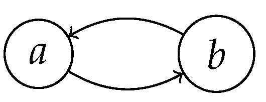
We associate with a dependence relation $\mathcal{D}$ on a finite set H a directed graph ${\mathsf{\Gamma }}_{\mathcal{D}}$ which has H as the set of its nodes and an edge goes from a to b if and only if $b\in {Infl}_d\left(a\right)$.

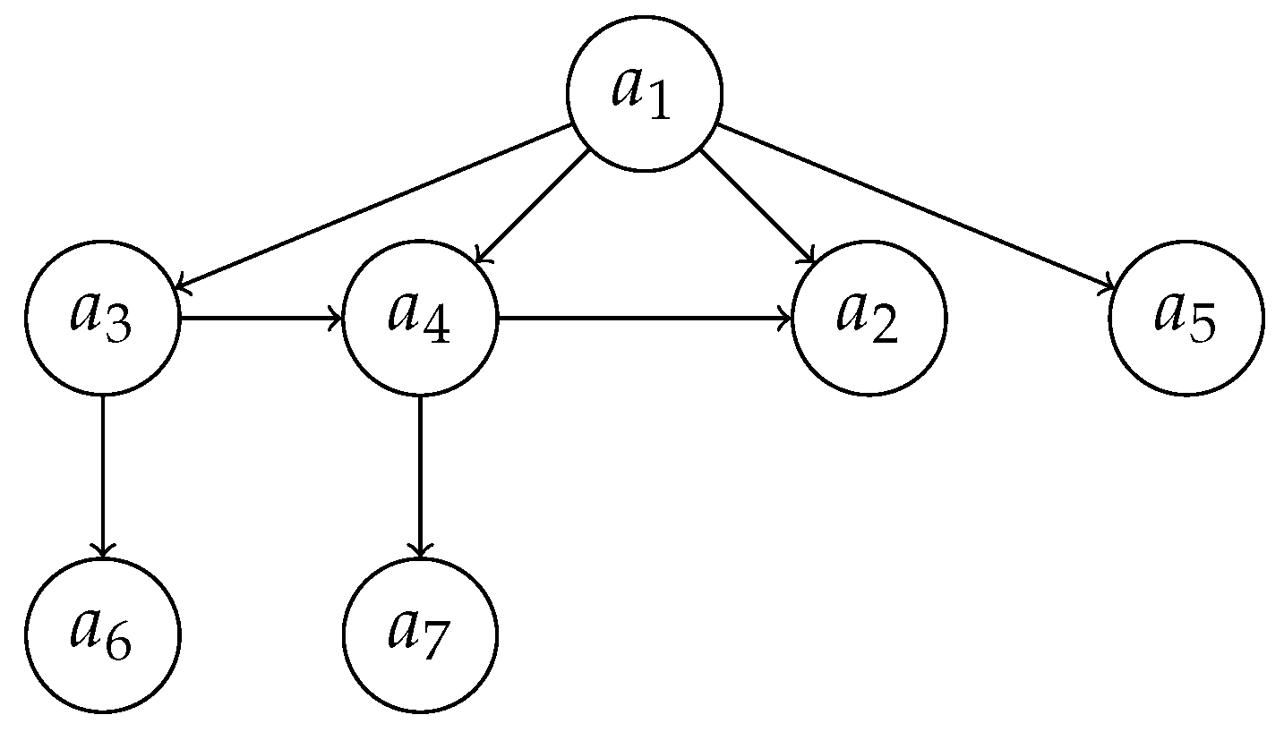
Example 1.

For the dependence relation in (2) we obtain the directed graph in Figure 1:

Note that the dependence relation (3) produces precisely the same directed graph as in the previous example.

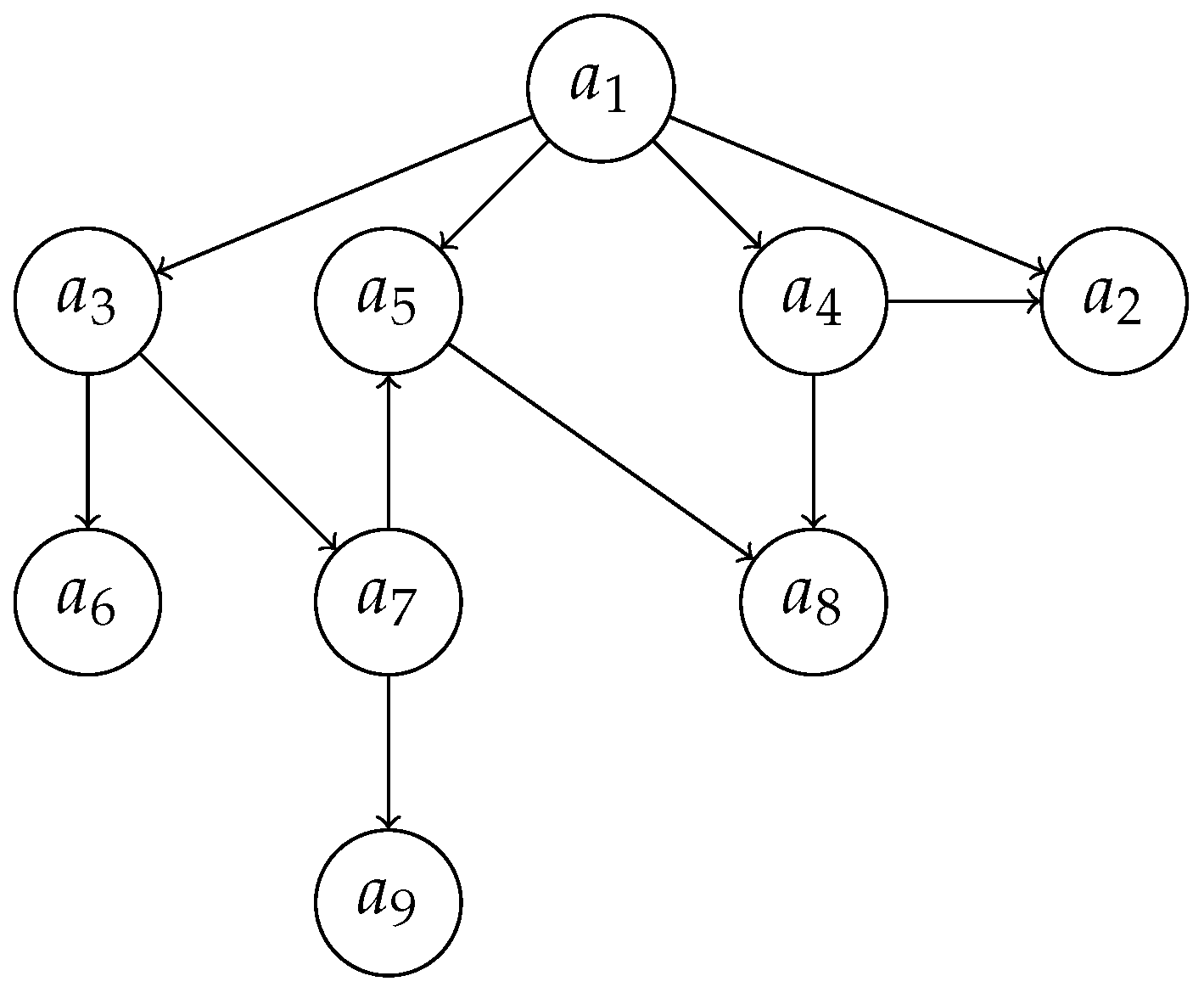
Example 2.

As a more complex example, let us consider the composed dependence relation:

$$a_1\sim D(a_2,a_3\sim D(a_6,a_7\sim D(a_5,a_9)),a_4\sim D(a_2,a_8),a_5\sim D\left(a_8\right)).$$

(5)

The directed graph associated with this dependence relation is represented in Figure 2.

Let us note that if each element belongs only to one level of influential elements, then we obtain a hierarchical graph used in neural networks or analytic hierarchy processes [3]. However, this might not happen for general dependence relations. There might indeed be two paths of different lengths leading from one node to another in the directed graph associated with a dependence relation.

4. The Influence Degree

The aim of this section is to define a degree that measures the influence of one element on another, with respect to a given dependence relation on a finite set. Given a dependence relation on a finite set H, we will first define a partial hyperoperation on H. For this, we found useful the concept of Corsini’s hyperoperation (see [29]) associated with a binary relation $R\subseteq H\times H$ on H, which is defined as:

$$\begin{array}{cc}\hfill {★}_R:H\times H& ⟶\mathcal{P}\left(H\right),\hfill \\ \hfill x{★}_{R}y=\{z\in H\mid (x,z)& \in R\mathrm{and}(z,y)\in R\}.\hfill \end{array}$$

The obtained hypercompositional structure $(H,{★}_R)$ is called Corsini’s partial hypergroupoid or partial C-hypergroupoid.

To associate a partial hyperoperation ${\circ }_{\mathcal{D}}:H\times H\to \mathcal{P}\left(H\right)$ with a dependence relation $\mathcal{D}$ on a finite set H, let us consider the following binary relation on H:

$$a{\le }_{\mathcal{D}}b\iff a\in Infl\left(b\right).$$

We used the symbol ≤ because of the following observation.

Lemma 2.

Let $\mathcal{D}$ be a dependence relation on a finite set H. The binary relation ${\le }_{\mathcal{D}}$ defined above is reflexive and transitive.

Proof. 

Reflexivity is a direct consequence of the fact that we consider any element of H as dependent on itself. For transitivity, let us assume that $a{\le }_{\mathcal{D}}b$ and $b{\le }_{\mathcal{D}}c$. That is, $a\in Infl\left(b\right)$ and $b\in Infl\left(c\right)$. If $n,m\in \mathbb{N}$ are such that $a\in {Infl}^n\left(b\right)$ and let $b\in {Infl}^m\left(c\right)$, then $a\in {Infl}^{n+m}\left(c\right)$ by Lemma 1. Therefore, $a\in Infl\left(c\right)$ and $a{\le }_{\mathcal{D}}c$.□

Remark 2.

The relation ${\le }_{\mathcal{D}}$ is not antisymmetric in general, as it can be observed in Example 5 below, where $a\ne a_5$ and $a_1{\le }_{\mathcal{D}}{a}_5{\le }_{\mathcal{D}}{a}_1$.

We let ${\circ }_{\mathcal{D}}$ be Corsini’s hyperoperation associated with ${\le }_{\mathcal{D}}$, i.e., ${\circ }_{\mathcal{D}}:={★}_{{\le }_{\mathcal{D}}}$.

In what follows, we give a graphical interpretation of ${\circ }_{\mathcal{D}}$ using the directed graph ${\mathsf{\Gamma }}_{\mathcal{D}}$.

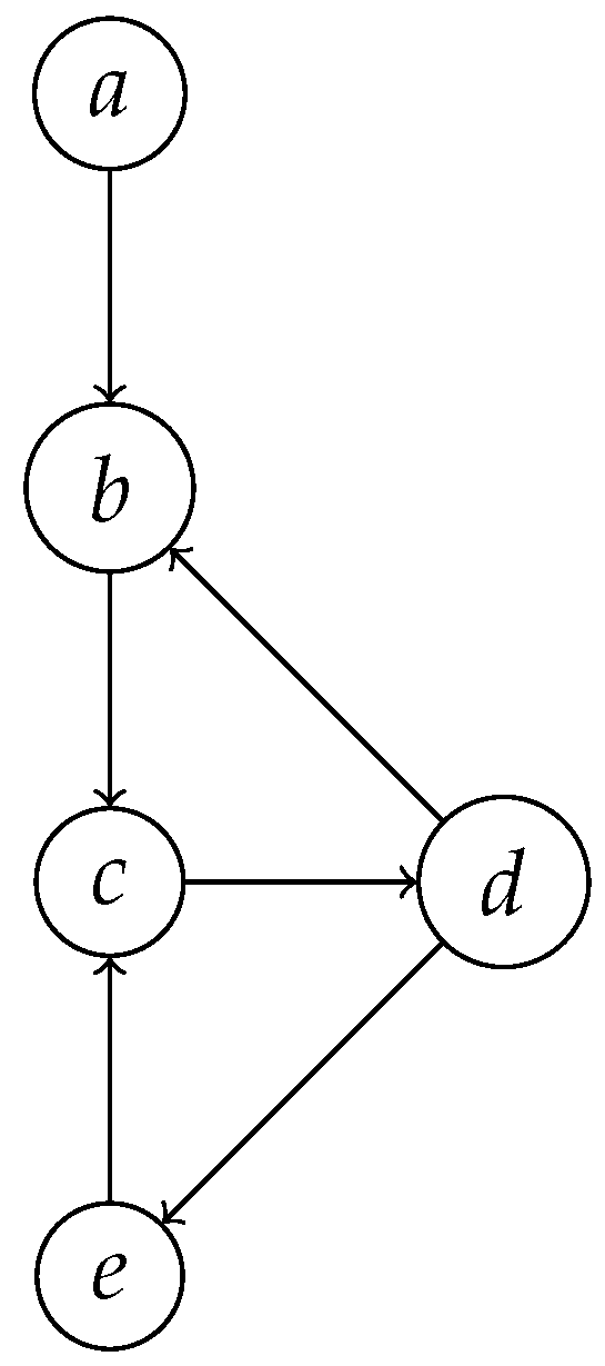
For a directed graph $\mathsf{\Gamma }$ and two nodes $a,b$ of $\mathsf{\Gamma }$, we denote by $P_{\mathsf{\Gamma }}(a,b)$ the set of all nodes that occur in some directed path from a to b. If a node b cannot be reached from node a, then $P_{\mathsf{\Gamma }}(a,b)=\varnothing$. Let us specify that in building a directed path, we may use any edge only once, while a node can be considered more times. For example, see the directed graph $\mathsf{\Gamma }$ in Figure 3.

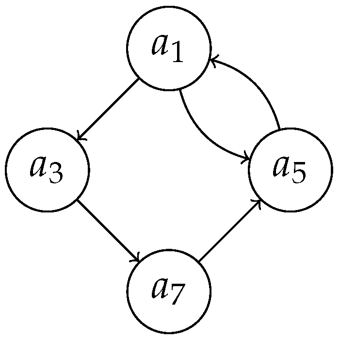
We have that $P_{\mathsf{\Gamma }}(a,b)=\{a,b,c,d\}$. Note that $e\notin P_{\mathsf{\Gamma }}(a,b)$ because we cannot find any path connecting a and b and passing through e without considering twice the edge $(c,d)$.

The following is a straightforward observation.

Lemma 3.

Let $\mathcal{D}$ be a dependence relation on a finite set H and let $\mathsf{\Gamma }={\mathsf{\Gamma }}_{\mathcal{D}}$ be the corresponding directed graph. Then $P_{\mathsf{\Gamma }}(a,b)=a{\circ }_{\mathcal{D}}b$.

Proof. 

Indeed, by definition of $\mathsf{\Gamma }$, we have that $c\in P_{\mathsf{\Gamma }}(a,b)$ if and only if $a\in Infl\left(c\right)$ and $c\in Infl\left(b\right)$, so by definition of ${\circ }_{\mathcal{D}}$ and ${\le }_{\mathcal{D}}$, we obtain that:

$$a{\circ }_{\mathcal{D}}b=\{c\in H\mid a{\le }_{\mathcal{D}}c{\le }_{\mathcal{D}}b\}=\{c\in H\mid a\in Infl\left(c\right)\mathrm{and}c\in Infl\left(b\right)\}=P_{\mathsf{\Gamma }}(a,b).$$

□

Remark 3.

Kalampakas et al. in [14] defined the path hyperoperation associated with a directed graph $\mathsf{\Gamma }=(V,E)$. It is easy to see that if $E\subseteq V\times V$ is reflexive and transitive, then the path hyperoperation induced by Γ and Corsini’s hyperoperation induced by the binary relation E coincide. Nevertheless, we want to stress that the directed graph ${\mathsf{\Gamma }}_{\mathcal{D}}$ associated with a dependence relation $\mathcal{D}$ has an edge $(a,b)$ if and only if $b\in {Infl}_d\left(a\right)$, while the hypeoperation ${\circ }_{\mathcal{D}}$ is Corsini’s hyperoperation associated with the binary relation $b{\le }_{\mathcal{D}}a$, i.e., $b\in Infl\left(a\right)$. Thus, ${\circ }_{\mathcal{D}}$ is not the path hyperoperation associated with ${\mathsf{\Gamma }}_{\mathcal{D}}$.

Definition 3.

Let $\mathcal{D}$ be a dependence relation on a finite set H. For $a,b\in H$ let $H^{\prime }:=b{\circ }_{\mathcal{D}}a$. We define the pre-degree of influence of a on b as

$$pre\text{-}deginfl(a,b):=\left\{\begin{array}{cc}0\hfill & if{H}^{\prime }=\varnothing ,\hfill \\ {\tilde{\mu }}_{(H^{\prime },\circ )}\left(b\right)\hfill & otherwise,\hfill \end{array}\right.$$

where ∘ denotes the restriction of the partial hyperoperation ${\circ }_{\mathcal{D}}$ to $H^{\prime }$.

Therefore, if $b{\circ }_{\mathcal{D}}a\ne \varnothing$, then

$$pre\text{-}deginfl(a,b)=\frac{1}{\left|Q\right(b\left)\right|}\sum _{(x,y)\in Q\left(b\right)}\frac{1}{|x{\circ }_{\mathcal{D}}y|}.$$

Graphically, to compute $pre\text{-}deginfl(a,b)$, we consider the subgraph $\mathsf{\Gamma }$ of ${\mathsf{\Gamma }}_{\mathcal{D}}$ consisting of all possible paths from b to a. Since an element always depends on itself, all graphs ${\mathsf{\Gamma }}_{\mathcal{D}}$ induced by a dependence relation $\mathcal{D}$ have loops on all of its nodes, which for simplicity we will omit in the pictures, but should be counted in building paths.

Example 3.

For the graph in Figure 2, we want to compute $pre\text{-}deginfl(a_7,a_1)$, and hence we consider the graph in Figure 4.

The partial hyperoperation associated with this graph has the following Cayley table:

∘	$a_1$	$a_3$	$a_7$
$a_1$	$\left\{a_1\right\}$	$\{a_1,a_3\}$	$\{a_1,a_3,a_7\}$
$a_3$	∅	$\left\{a_3\right\}$	$\{a_3,a_7\}$
$a_7$	∅	∅	$\left\{a_7\right\}$

Therefore,

$$\begin{array}{cc}\hfill Q\left(a_1\right)& =\{(a_1,a_1),(a_1,a_3),(a_1,a_7)\}\hfill \\ \hfill q\left(a_1\right)& =3\hfill \\ \hfill pre\text{-}deginfl(a_7,a_1)=\tilde{\mu }\left(a_1\right)& =\frac{1}{3}·\left(1+\frac{1}{2}+\frac{1}{3}\right)=\frac{11}{18}\approx 0.61.\hfill \end{array}$$

Since in the graph in Figure 2 there are no directed paths from $a_7$ to $a_1$, we have that

$$pre\text{-}deginfl(a_1,a_7)=0.$$

Example 4.

Consider again the graph from Figure 2. We want to determine the pre-degree of influence of $a_5$ on $a_1$. So we will consider the subgraph in Figure 5.

The partial hyperoperation associated with this graph has the following Cayley table:

∘	$a_1$	$a_3$	$a_5$	$a_7$
$a_1$	$\left\{a_1\right\}$	$\{a_1,a_3\}$	$\{a_1,a_3,a_5,a_7\}=H$	$\{a_1,a_3,a_7\}$
$a_3$	∅	$\left\{a_3\right\}$	$\{a_3,a_5,a_7\}$	$\{a_3,a_7\}$
$a_5$	∅	∅	$\left\{a_5\right\}$	∅
$a_7$	∅	∅	$\{a_5,a_7\}$	$\left\{a_7\right\}$

and we have that

$$\begin{array}{cc}\hfill Q\left(a_1\right)& =\{(a_1,a_1),(a_1,a_3),(a_1,a_7),(a_1,a_5)\}\hfill \\ \hfill q\left(a_1\right)& =4\hfill \\ \hfill A\left(a_1\right)=\sum _{a_1\in x\circ y}\frac{1}{|x\circ y|}& =1+\frac{1}{2}+\frac{1}{3}+\frac{1}{4}=\frac{12+6+4+3}{12}=\frac{25}{12}\hfill \\ \hfill pre\text{-}deginfl(a_5,a_1)=\tilde{\mu }\left(a_1\right)& =\frac{25}{48}\approx 0.52.\hfill \end{array}$$

Example 5.

Consider the dependence relation

$$a_1\sim D(a_2,a_3\sim D(a_6,a_7\sim D(a_5,a_9)),a_4\sim D(a_2,a_8),a_5\sim D(a_1,a_8))$$

(6)

whose associated graph can be obtained from the graph in Figure 2 with the addition of the edge $(a_5,a_1)$. We now show by direct computations that the pre-degree of influence of $a_5$ on $a_1$ decreases. The corresponding subgraph is the one in Figure 6.

The partial hyperoperation associated with this graph has the following Cayley table:

∘	$a_1$	$a_3$	$a_5$	$a_7$
$a_1$	$\{a_1,a_3,a_5,a_7\}$	$\{a_1,a_3,a_5\}$	$\{a_1,a_3,a_5,a_7\}$	$\{a_1,a_3,a_5,a_7\}$
$a_3$	$\{a_1,a_3,a_5,a_7\}$	$\{a_1,a_3,a_5,a_7\}$	$\{a_1,a_3,a_5,a_7\}$	$\{a_3,a_7\}$
$a_5$	$\{a_1,a_5\}$	$\{a_1,a_3,a_5\}$	$\{a_1,a_3,a_5,a_7\}$	$\{a_1,a_3,a_5,a_7\}$
$a_7$	$\{a_1,a_5,a_7\}$	$\{a_1,a_3,a_5,a_7\}$	$\{a_1,a_5,a_7\}$	$\{a_1,a_3,a_5,a_7\}$

Note that since the graph contains a cycle connecting all nodes, we do not have empty values and $a_i{\circ }_{\mathcal{D}}{a}_i=\{a_1,a_3,a_5,a_7\}=:H$. Similarly, having the path $a_3-a_7-a_5-a_1-a_5$, we have $a_3{\circ }_{\mathcal{D}}{a}_5=H$. Therefore,

$$\begin{array}{cc}\hfill Q\left(a_1\right)& =H\times H\setminus \left\{(a_3,a_7)\right\}\hfill \\ \hfill q\left(a_1\right)& =15\hfill \\ \hfill A\left(a_1\right)=\frac{10}{4}+\frac{4}{3}+\frac{1}{2}& =\frac{52}{12}\hfill \\ \hfill pre\text{-}deginfl(a_5,a_1)=\tilde{\mu }\left(a_1\right)& =\frac{52}{12·15}\approx 0.28.\hfill \end{array}$$

In the last two examples (see also Example 8 below), the edge $(a_1,a_5)$ gives no contribution to the value of the pre-degree of influence. That is because the partial hyperoperation ${\circ }_{\mathcal{D}}$ is based on a transitive binary relation, and the edges $(a_1,a_3),(a_3,a_7)$ and $(a_7,a_5)$ imply $a_1{\le }_{\mathcal{D}}{a}_5$ while they do not imply the existence of the edge $(a_1,a_5)$. From the point of view of our interpretation, this is a problem because the edge $(a_1,a_5)$ indicates that $a_5$ is a direct influential element of $a_1$ and thus has a stronger influence. Our definition of the degree of influence is based on the pre-degree of influence but needs a further step in order to improve its sensibility in similar cases. In this setting, both our graphical method and the hyperoperation ${\circ }_{\mathcal{D}}$ become necessary.

Let $\mathsf{\Gamma }$ be a directed graph and P be a directed path in $\mathsf{\Gamma }$. We define the length of P to be the number of its nodes and denote it by $\ell \left(P\right)$. If a and b are nodes of $\mathsf{\Gamma }$, we denote by $\mathfrak{p}(a,b)$ the set of paths from a to b.

Definition 4.

Let $\mathcal{D}$ be a dependence relation on a finite set H. For $a,b\in H$ let $H^{\prime }:=b{\circ }_{\mathcal{D}}a$. We define the degree of influence of a on b as 0 if $H^{\prime }=\varnothing$, otherwise

$$deginfl(a,b):=\frac{1}{\left|Q\right(b\left)\right|}\left(\sum _{(x,y)\in Q\left(b\right)}\frac{1}{\left|\mathfrak{p}\right(x,y\left)\right|}\sum _{P\in \mathfrak{p}(x,y)}\frac{1}{\ell \left(P\right)}\right).$$

where $Q\left(b\right)=\{(x,y)\in H^{\prime }\times H^{\prime }\mid b\in x{\circ }_{\mathcal{D}}y\}$.

The following result is a direct consequence of the definitions.

Proposition 2.

Let $\mathcal{D}$ be a dependence relation on a finite set H and $a,b\in H$ such that $b{\circ }_{\mathcal{D}}a\ne \varnothing$. Then

$$pre\text{-}deginfl(a,b)\le deginfl(a,b)$$

with equality holding if and only if $\left|\mathfrak{p}\right(b,a\left)\right|=1$.

Proof. 

Take $a,b\in H$ such that $H^{\prime }:=b{\circ }_{\mathcal{D}}a\ne \varnothing$. Let $x,y\in H^{\prime }$ be such that $b\in x{\circ }_{\mathcal{D}}y$. Since $|x{\circ }_{\mathcal{D}}y|=|P_{{\mathsf{\Gamma }}_{\mathcal{D}}}(x,y)|$ (Lemma 3) is the number of nodes on all paths from x to y and if $P\in \mathfrak{p}(x,y)$, then $\ell \left(P\right)$ is the number of nodes on the path P from x to y, and we obtain that $|x{\circ }_{\mathcal{D}}y|\ge \ell \left(P\right)$ for all $P\in \mathfrak{p}(x,y)$ and therefore

$$1\le \frac{1}{\left|\mathfrak{p}\right(x,y\left)\right|}\sum _{P\in \mathfrak{p}(x,y)}\frac{|x{\circ }_{\mathcal{D}}y|}{\ell \left(P\right)}=\frac{|x{\circ }_{\mathcal{D}}y|}{\left|\mathfrak{p}\right(x,y\left)\right|}\sum _{P\in \mathfrak{p}(x,y)}\frac{1}{\ell \left(P\right)}$$

and then

$$\frac{1}{|x{\circ }_{\mathcal{D}}y|}\le \frac{1}{\left|\mathfrak{p}\right(x,y\left)\right|}\sum _{P\in \mathfrak{p}(x,y)}\frac{1}{\ell \left(P\right)}.$$

Thus, we have that

$$\begin{array}{cc}\hfill pre\text{-}deginfl(a,b)& =\frac{1}{\left|Q\right(b\left)\right|}\sum _{(x,y)\in Q\left(b\right)}\frac{1}{|x{\circ }_{\mathcal{D}}y|}\hfill \\ \hfill & \le \frac{1}{\left|Q\right(b\left)\right|}\left(\sum _{(x,y)\in Q\left(b\right)}\frac{1}{\left|\mathfrak{p}\right(x,y\left)\right|}\sum _{P\in \mathfrak{p}(x,y)}\frac{1}{\ell \left(P\right)}\right)\hfill \\ \hfill & =deginfl(a,b).\hfill \end{array}$$

□

Let us now consider further examples.

Example 6.

Consider again the dependence relation $\mathcal{D}$ from (5). To compute $deginfl(a_5,a_1)$, we extract the subgraph of ${\mathsf{\Gamma }}_{\mathcal{D}}$ that we drew in Figure 5. When filling the Cayley table of the partial hyperoperation ${\circ }_{\mathcal{D}}$, we now keep track of all the possible paths and list them in the corresponding cell:

	$a_1$	$a_3$	$a_5$	$a_7$
$a_1$	$\left\{a_1\right\}$	$\{a_1,a_3\}$	$\{a_1,a_3,a_7,a_5\}$, $\{a_1,a_5\}$	$\{a_1,a_3,a_7\}$
$a_3$	∅	$\left\{a_3\right\}$	$\{a_3,a_5,a_7\}$	$\{a_3,a_7\}$
$a_5$	∅	∅	$\left\{a_5\right\}$	∅
$a_7$	∅	∅	$\{a_5,a_7\}$	$\left\{a_7\right\}$

We now compute the degree of influence:

$$deginfl(a_5,a_1)=\frac{1}{4}\left(1+\frac{1}{2}+\frac{1}{3}+\frac{1}{2}\left(\frac{1}{4}+\frac{1}{2}\right)\right)=\frac{53}{96}\approx 0.552.$$

The reader can note that $deginfl(a_5,a_1)>pre\text{-}deginfl(a_5,a_1)$ in this case.

Example 7.

Consider now the dependence relation (6). The subgraph of paths from $a_1$ to $a_5$ is in Figure 6. The table to compute $deginfl(a_5,a_1)$ is:

	$a_1$	$a_3$	$a_5$	$a_7$
$a_1$	$\{a_1,a_3,a_5,a_7\}$	$\{a_1,a_3,a_5\}$	$\{a_1,a_3,a_5,a_7\}$, $\{a_1,a_5\}$	$\{a_1,a_3,a_5,a_7\}$
$a_3$	$\{a_1,a_3,a_5,a_7\}$	$\{a_1,a_3,a_5,a_7\}$	$\{a_3,a_5,a_7\}$, $\{a_1,a_3,a_5,a_7\}$	$\{a_3,a_7\}$
$a_5$	$\{a_1,a_5\}$	$\{a_1,a_3,a_5\}$	$\{a_1,a_5\}$, $\{a_1,a_3,a_5,a_7\}$	$\{a_1,a_3,a_5,a_7\}$
$a_7$	$\{a_1,a_5,a_7\}$	$\{a_1,a_3,a_5,a_7\}$	$\{a_5,a_7\}$, $\{a_1,a_5,a_7\}$	$\{a_1,a_3,a_5,a_7\}$

which comes from the graph in Figure 6. Therefore, in this case:

$$deginfl(a_5,a_1)=\frac{1}{15}\left(\frac{7}{4}+\frac{3}{3}+\frac{1}{2}+\left(\frac{1}{4}+\frac{1}{2}\right)+\frac{1}{2}\left(\frac{1}{2}+\frac{1}{4}\right)+\frac{1}{2}\left(\frac{1}{2}+\frac{1}{3}\right)\right)=\frac{113}{360}\approx 0.31.$$

The reader can note that $deginfl(a_5,a_1)>pre\text{-}deginfl(a_5,a_1)$ in this case.

Let us now compare dependence relations that are similar to one another.

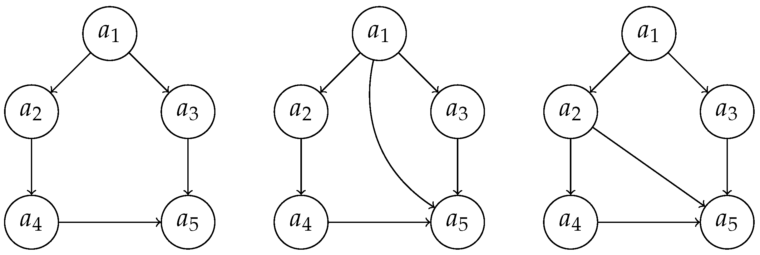
Example 8.

Let us compare the degree of influence of $a_5$ on $a_1$ for the following three dependence relations:

$$a_1\sim D(a_2\sim D(a_4\sim D\left(a_5\right)),a_3\sim D\left(a_5\right))$$

(7)

$$a_1\sim D(a_2\sim D(a_4\sim D\left(a_5\right)),a_3\sim D\left(a_5\right),a_5)$$

(8)

$$a_1\sim D(a_2\sim D(a_4\sim D\left(a_5\right),a_5),a_3\sim D\left(a_5\right)).$$

(9)

The corresponding graphs are those in Figure 7.

For the dependence relation (7), we find the table:

∘	$a_1$	$a_2$	$a_3$	$a_4$	$a_5$
$a_1$	$\left\{a_1\right\}$	$\{a_1,a_2\}$	$\{a_1,a_3\}$	$\{a_1,a_2,a_4\}$	$\{a_1,a_2,a_4,a_5\}$, $\{a_1,a_3,a_5\}$
$a_2$	∅	$\left\{a_2\right\}$	∅	$\{a_2,a_4\}$	$\{a_2,a_4,a_5\}$
$a_3$	∅	∅	$\left\{a_3\right\}$	∅	$\{a_3,a_5\}$
$a_4$	∅	∅	∅	$\left\{a_4\right\}$	$\{a_4,a_5\}$
$a_5$	∅	∅	∅	∅	$\left\{a_5\right\}$

which yields:

$$deginfl(a_5,a_1)=\frac{1}{5}\left(1+\frac{1}{2}+\frac{1}{2}+\frac{1}{3}+\frac{1}{2}\left(\frac{1}{4}+\frac{1}{3}\right)\right)=\frac{21}{40}=0.525.$$

For the dependence relation (8), we find the table:

∘	$a_1$	$a_2$	$a_3$	$a_4$	$a_5$
$a_1$	$\left\{a_1\right\}$	$\{a_1,a_2\}$	$\{a_1,a_3\}$	$\{a_1,a_2,a_4\}$	$\{a_1,a_2,a_4,a_5\}$, $\{a_1,a_3,a_5\}$, $\{a_1,a_5\}$
$a_2$	∅	$\left\{a_2\right\}$	∅	$\{a_2,a_4\}$	$\{a_2,a_4,a_5\}$
$a_3$	∅	∅	$\left\{a_3\right\}$	∅	$\{a_3,a_5\}$
$a_4$	∅	∅	∅	$\left\{a_4\right\}$	$\{a_4,a_5\}$
$a_5$	∅	∅	∅	∅	$\left\{a_5\right\}$

which yields:

$$deginfl(a_5,a_1)=\frac{1}{5}\left(1+\frac{1}{2}+\frac{1}{2}+\frac{1}{3}+\frac{1}{3}\left(\frac{1}{2}+\frac{1}{4}+\frac{1}{3}\right)\right)=\frac{97}{180}\approx 0.538.$$

For the dependence relation (9), we find the table:

∘	$a_1$	$a_2$	$a_3$	$a_4$	$a_5$
$a_1$	$\left\{a_1\right\}$	$\{a_1,a_2\}$	$\{a_1,a_3\}$	$\{a_1,a_2,a_4\}$	$\{a_1,a_2,a_4,a_5\}$, $\{a_1,a_3,a_5\}$, $\{a_1,a_2,a_5\}$
$a_2$	∅	$\left\{a_2\right\}$	∅	$\{a_2,a_4\}$	$\{a_2,a_5\}$,$\{a_2,a_4,a_5\}$
$a_3$	∅	∅	$\left\{a_3\right\}$	∅	$\{a_3,a_5\}$
$a_4$	∅	∅	∅	$\left\{a_4\right\}$	$\{a_4,a_5\}$
$a_5$	∅	∅	∅	∅	$\left\{a_5\right\}$

which yields

$$deginfl(a_5,a_1)=\frac{1}{5}\left(1+\frac{1}{2}+\frac{1}{2}+\frac{1}{3}+\frac{1}{3}\left(\frac{1}{3}+\frac{1}{4}+\frac{1}{3}\right)\right)=\frac{19}{36}\approx 0.527.$$

Note that in all three cases above, we have that:

$$pre\text{-}deginfl(a_5,a_1)=\frac{1}{5}\left(1+\frac{1}{2}+\frac{1}{2}+\frac{1}{3}+\frac{1}{5}\right)=\frac{38}{75}\approx 0.506.$$

The degree of influence of an element on another can be arbitrarily small.

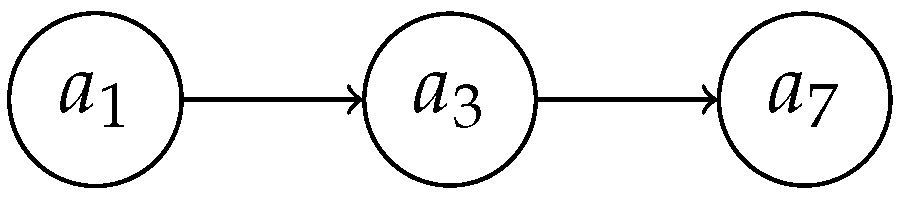
Theorem 1.

For any $0<\epsilon <1$, there is a dependence relation $\mathcal{D}$ on a finite set H and $a,b\in H$ such that $deginfl(a,b)<\epsilon$.

Proof. 

Let $n\in \mathbb{N}$. We consider the composed dependence relation $\mathcal{D}$ on $H:=\{a_1,\dots ,a_n\}$ given by the composition of the dependence relations

$$a_i\sim D\left(a_{i+1}\right)(1\le i\le n).$$

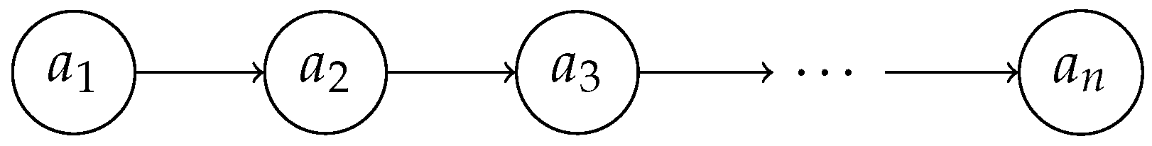
The directed graph corresponding to this composed dependence relation is the one represented in Figure 8.

Thus, we have that

$$deginfl(a_n,a_1)=pre\text{-}deginfl(a_n,a_1)=\frac{1}{n}·\sum _{k=1}^n\frac{1}{k}$$

and

$$\underset{n\to \infty }{lim}deginfl(a_n,a_1)=0.$$

can be shown using elementary methods. This completes the proof of the theorem.□

The dependence relations inducing a linear graph have an interesting symmetry.

Proposition 3.

If we consider the dependence relations ${\mathcal{D}}_1$, ${\mathcal{D}}_2$, which correspond to the graphs obtained from the linear graph in Figure 6 with the addition of one edge $(a_m,a_k)$ with $k>m+1$ or with the addition of the edge $(a_m,a_{n-k+m+2})$, then ${deginfl}_{{\mathcal{D}}_1}(a_n,a_1)={deginfl}_{{\mathcal{D}}_2}(a_n,a_1)$.

Proof. 

We can assume without loss of generality that $m=1$. Then, by properly arranging the terms of the sums, we obtain that

$$\begin{array}{cc}\hfill {deginfl}_{{\mathcal{D}}_1}(a_n,a_1)& =\frac{1}{n}\left(1+\dots +\frac{1}{k-1}+\frac{1}{2}\left(\frac{1}{2}+\frac{1}{k}\right)+\dots +\frac{1}{2}\left(\frac{1}{n-k+1}+\frac{1}{n}\right)\right)\hfill \\ \hfill & =\frac{1}{n}\left(1+\dots +\frac{1}{n-k+2}+\frac{1}{2}\left(\frac{1}{2}+\frac{1}{n-k+3}\right)+\dots +\frac{1}{2}\left(\frac{1}{k-2}+\frac{1}{n}\right)\right)\hfill \\ \hfill & ={deginfl}_{{\mathcal{D}}_2}(a_n,a_1).\hfill \end{array}$$

□

Example 9.

As an example we consider the dependence relations

$$D_1:a_1\sim D(a_2\sim D(a_3\sim D(a_4\sim D(a_5\sim D\left(a_6\right)))),a_6)$$

and

$$D_2:a_1\sim D(a_2\sim D(a_3\sim D(a_4\sim D(a_5\sim D\left(a_6\right)))),a_3).$$

The corresponding graphs are represented in Figure 9.

We have that

$$\begin{array}{cc}\hfill {deginfl}_{{\mathcal{D}}_1}(a_6,a_1)& =\frac{1}{6}\left(1+\frac{1}{2}+\frac{1}{3}+\frac{1}{4}+\frac{1}{5}+\frac{1}{2}\left(\frac{1}{2}+\frac{1}{6}\right)\right)\hfill \\ \hfill & =\frac{1}{6}\left(1+\frac{1}{2}+\frac{1}{3}+\frac{1}{4}+\frac{1}{5}+\frac{1}{4}+\frac{1}{12}\right)\hfill \\ \hfill & =\frac{1}{2}\left(1+\frac{1}{2}+\frac{1}{2}\left(\frac{1}{2}+\frac{1}{3}\right)+\frac{1}{2}\left(\frac{1}{3}+\frac{1}{4}\right)+\frac{1}{2}\left(\frac{1}{4}+\frac{1}{5}\right)+\frac{1}{2}\left(\frac{1}{5}+\frac{1}{6}\right)\right)\hfill \\ \hfill & ={deginfl}_{{\mathcal{D}}_2}(a_6,a_1).\hfill \end{array}$$

The next result shows that the degree of influence of an element on another cannot be higher than $0.75$.

Theorem 2.

Let H be a finite set. For all dependence relations on H and all $a,b\in H$, we have that

$$a\ne b⟹deginfl(a,b)\le \frac{3}{4}.$$

The maximum value of $deginfl(a,b)$ is achieved only by the dependence relation $b\sim D\left(a\right)$.

Proof. 

Let $\mathcal{D}$ be any dependence relation on a finite set H and take $a,b\in H$ with $a\ne b$. If $deginfl(a,b)=0$, then there is nothing to show. Otherwise,

$$deginfl(a,b)=\frac{1}{\left|Q\right(b\left)\right|}\left(\sum _{(x,y)\in Q\left(b\right)}\frac{1}{\left|\mathfrak{p}\right(x,y\left)\right|}\sum _{P\in \mathfrak{p}(x,y)}\frac{1}{\ell \left(P\right)}\right).$$

Note that for any $(x,y)\in Q\left(b\right)$ such that $x\ne y$ and any $P\in \mathfrak{p}(x,y)$, we have that $\ell \left(P\right)\ge 2$ since $x,y\in P$. Moreover, if $\ell \left(P\right)=1$, then $x=y=b$ must hold. It follows that

$$deginfl(a,b)\le \frac{1+\frac{r-1}{2}}{r}=\frac{1+r}{2r},$$

where

$$r:=\left|Q\left(b\right)\right|\prod _{(x,y)\in Q\left(b\right)}\left|\mathfrak{p}(x,y)\right|.$$

Since $(b,b),(b,a)\in Q\left(b\right)$, the assumption $a\ne b$ implies that $\left|Q\right(b\left)\right|\ge 2$ and thus $r\ge 2$. As the function $f\left(r\right)=(1+r)/2r$ is decreasing on $[2,+\infty )$, its maximum is achieved at $r=2$. We conclude that

$$deginfl(a,b)\le \frac{1+2}{2·2}=\frac{3}{4}$$

which completes the proof of the first statement of the theorem. The second statement is straightforward to verify.□

Let us prove that the influence degree satisfies all the desirable properties that we have listed in Section 3.

Theorem 3.

Let H be a finite set. For all dependence relations on H and all $a,b\in H$, we have that

(i)

$deginfl(a,b)\in [0,1]$;

(ii)

if $deginfl(a,b)=1$, then $a=b$;

(iii)

$deginfl(a,b)=0$ if and only if $a\notin Infl\left(b\right)$;

(iv)

if $a_1\in {Infl}_d\left(b\right)\setminus {Infl}_i\left(b\right)$ and $a_2\in {Infl}_i\left(b\right)\setminus {Infl}_d\left(b\right)$, then $deginfl(a_1,b)>deginfl(a_2,b)$.

Proof. 

Property $\left(i\right)$ is true by definition, and property $\left(ii\right)$ is an immediate corollary of Theorem 2. For $\left(iii\right)$, assume first that $a\notin Infl\left(b\right)$. Then $a\nleqq {\le }_{\mathcal{D}}b$, and it follows that $b{\circ }_{\mathcal{D}}a=\varnothing$, so $deginfl(a,b)=0$. Conversely, if $a\in Infl\left(b\right)$, then $a{\le }_{\mathcal{D}}b$ and thus $H^{\prime }:=b{\circ }_{\mathcal{D}}a\ne \varnothing$. Now, since $a\in a{\circ }_{\mathcal{D}}a$, it follows that $Q\left(a\right)\ne \varnothing$ in $(H^{\prime },{\circ }_{\mathcal{D}})$, and it follows that $deginfl(a,b)\ne 0$. Property $\left(iv\right)$ is a direct consequence of Theorem 2.□

Example 10.

As an example, let us compute some degrees of influence in some cases arising from the dependence relation of Example 2 above, which can help the reader verify the properties listed in the statements of the above theorems.

As we have already observed in Example 3 for the pre-degree of influence, we obtain that $deginfl(a_1,a_7)=0$. This follows from the fact that there are no directed paths from $a_7$ to $a_1$ in the graph of Figure 2.

The element $a_3$ has a maximal degree of influence on $a_1$, as it is a direct influential element of $a_1$. Indeed, to compute $deginfl(a_3,a_1)$, we consider the directed graph represented in Figure 10.

and we obtain that

$$deginfl(a_3,a_1)=\frac{1}{2}\left(1+\frac{1}{2}\right)=\frac{3}{4}.$$

Note that $a_5$ is also a direct influential element of $a_1$, but it is also an influential element of $a_1$ of level 3. As a consequence, we obtain that

$$deginfl(a_5,a_1)=\frac{1}{4}\left(1+\frac{1}{2}+\frac{1}{3}+\frac{1}{2}\left(\frac{1}{2}+\frac{1}{4}\right)\right)=\frac{53}{96}<\frac{3}{4}.$$

For any indirect influential element of $a_1$ that is not a direct influential element, such as $a_9$, we obtain that

$$deginfl(a_9,a_1)=\frac{1}{4}\left(1+\frac{1}{2}+\frac{1}{3}+\frac{1}{4}\right)=\frac{25}{48}<\frac{3}{4}.$$

Since the only path in the directed graph in Figure 2 from $a_1$ to $a_1$ that does not use any edge two times consists of the loop $(a_1,a_1)$ alone, we obtain that $deginfl(a_1,a_1)=1$. Observe that $deginfl(x,x)=1$ does not always hold as in the presence of a cycle, the degree of influence of an element on itself can be less than 1. Consider, for example, the graph in Figure 11.

We obtain that

$$deginfl(a,a)=\frac{1}{2}\left(\frac{1}{2}\left(1+\frac{1}{2})+\frac{1}{2}\right)\right)=\frac{5}{8}<1.$$

Our interpretation of this last fact is that, being part of a cycle of dependences, the element under consideration is not able to fully influence itself as its actions to pursue a certain influence on itself, after going through the cycle, may result in a response that prevents this influence.

5. Conclusions and Open Problems

Hypercompositional algebra seems to be a suitable tool for modelling several applicative aspects, one of them being the interrelations and dependences among several variables. Another similar application of this theory is presented in [30], by modelling of trajectories in HD maps, as well as in [31] when the environment of the binary state machines are represented by hypergroups.

The procedure that we have described in this paper aims to measure the degree of influence of an element on another with respect to a given dependence relation on a finite set. On the one hand, the definition is inspired by ideas of Corsini to construct a fuzzy set from a (partial) hypergroupoid which we associate with any dependence relation. On the other hand, representing the dependence relation by a directed graph has revealed a necessary step as well.

The computations presented in our examples show that the degree of influence is generally well-behaved in the sense that the values it takes match the expectations we have from our interpretation of dependence relations. Nevertheless, computations can become very complex when the cardinality of the considered set H gets large. In the future, we aim to find general results supporting our feeling that the degree of influence is a good model for real-world inter-dependences. For concrete applications, we found inspiration, e.g., in [32]. In addition, we believe that finding more symmetries as in Proposition 3 above can help to smooth the computations on large sets and elaborate effective algorithms to perform them.