Extinction and Ergodic Stationary Distribution of COVID-19 Epidemic Model with Vaccination Effects

Abstract

Human society always wants a safe environment from pollution and infectious diseases, such as COVID-19, etc. To control COVID-19, we have started the big effort for the discovery of a vaccination of COVID-19. Several biological problems have the aspects of symmetry, and this theory has many applications in explaining the dynamics of biological models. In this research article, we developed the stochastic COVID-19 mathematical model, along with the inclusion of a vaccination term, and studied the dynamics of the disease through the theory of symmetric dynamics and ergodic stationary distribution. The basic reproduction number is evaluated using the equilibrium points of the proposed model. For well-posedness, we also test the given problem for the existence and uniqueness of a non-negative solution. The necessary conditions for eradicating the disease are also analyzed along with the stationary distribution of the proposed model. For the verification of the obtained result, simulations of the model are performed.

1. Introduction

For the control and extinction of COVID-19, several effective measurements have been taken from many researchers and policymakers of each country of the globe. Many of them are very economical and have produced a disturbance in the routine activities of social media and psychological effects. Controlling of the said disease viruses for all people showing signs of infection or not is the significant and key work of the higher-ups and managerial staff. Still now in the process of developing safety against COVID-19, the most important tool is vaccination [1,2]. This infection may spread through human-to-human contact in the society, like (MERS-CoV), which is transmitted from civet cats into the human environment. Various efforts have been made against it, which can be studied in [3,4].

The mathematical formulation may well present the dynamical behavior of the infectious diseases of different epidemics. Therefore, different approaches of mathematical modeling for the biological dynamics have been used in the past history. Among them is deterministic mathematical modeling, which mostly discusses the idealistic situation of real-world problems. It depends on input and output data. The stochastic modeling is another approach which mostly describes the real situation. It presents both the randomness of various compositions with division and also the deterministic version. Because of the noise terms as an input source, the said division may have dynamics of uncertainty [5,6,7,8].

So, for vaccination, the conversion of real global problems into mathematical terms is a very significant tool for the analysis of epidemics. Epidemiological infections are transferred through mathematical formulation to various types of differential equations and systems of it. Policy makers and many other scholars also provide some ideas and parameters which can be used for reducing infections [9]. From the beginning of the twenty-first century, the conversion of real-world problems to mathematical terms made the information very easy and made the situation very simple regarding future predictions [10,11]. Mostly, the infections are written in mathematical formulation. Different mathematical formulation are applied to mostly infectious diseases. The techniques of mathematical modeling are divided into different mechanisms. Among them are the deterministic, stochastic and difference equations. The stochastic-type approach is much more realistic as compared to other mechanisms of mathematical formulations. Such a scheme type gives the result in the form of up and down for unknown quantities along with the distribution of an approximate solution [10,11,12,13]. For such dynamics, one can study different articles, such as that given in reference [14,15].

The stochastic analysis of real-world phenomena is very good, as it involves both the input and output of the data of that responsible for the transmission of the disease. Due to this, it answers all questions related to infectious disease modeling. It discusses how to construct a mathematical model for infectious disease. It also answers the question of how to formulate the intermediate frequently transmitted disease. The rate of disease and its suitable position in the model is also discussed by the stochastic approach. So for the need of these points, we formulate the COVID-19 problem by the mathematical term of stochastic approach. Changing the densities of different model quantities, we construct the model for the said infection with a long period of time investigation.

Several biological problems have the aspects of symmetry, and this theory has many applications in explaining the dynamics of biological models. The systematic theory of symmetry has several applications in the development and study of models of biological shapes and phenomena. In engineering and physics, symmetries are frequently accurate or nearly so, whereas in the biological sciences, perfect symmetry is uncommon. Because symmetries are only approximations in most biological systems, their application in models is an idealization. This type of idealization is beneficial because it simplifies the mathematical analysis and also because systems with approximated symmetries frequently reflect idealized symmetric models more precisely than ordinary asymmetric ones. The symmetrical methods are especially suited in biological environments where somewhat consistent patterns are found.

The analysis of symmetry features of ODEs and PDEs is a popular and well-established topic (see [16,17]) and provides a valuable tool for better comprehension of the solution’s qualitative behavior. In contrast, a similar theory of SDE symmetries was just recently constructed; the readers are suggested to see [18,19,20]. In this work, we studied a stochastic COVID-19 model by using a very general and elegant approach for solving a SDE via symmetries in a dynamical perspective. Unfortunately, the scale and complexity of many models in mathematical biology renders a brute force application of symmetry methods impractical. In other words, the analysis of SDEs using symmetry methods is non-standard in mathematical biology; thus, we will focus mainly on other available techniques for SDEs and will give less attention to the underlying symmetry methods.

The remaining part of this research paper is organized as follows: In Section 2, we develop the COVID-19 mathematical formulation with stochastic fluctuation in the rate of infection. In Section 3, we present the qualitative analysis of a non-negative solution for a long duration of time to the proposed stochastic model. We give some important conditions for the COVID-19 infection to vanish it from the society in Section 4. In Section 6, the condition for the stationary distribution existence is provided. The scheme of the analytical solution and their graphical representation are given in Section 7. For the interested reader, we conclude the article with some future remarks in Section 8.

2. Models Formulation

The virus of COVID-19 has a proper incubation period and will result in confinement in the beginning from the community and after the detection of disease. Healthy individuals will have an incubation duration before disease onset. We construct the COVID-19 model with five ordinary equations of derivative. The quantities of the model are composed of Susceptible $\left(\mathbb{S}\right)$, Immunize or Vaccinated $\left(\mathbb{V}\right)$, Asymptomatic or Exposed $\left(\mathbb{E}\right)$, Symptomatic or Infectious $\left(\mathbb{I}\right)$, hospitalized $\left(\mathbb{H}\right)$, and recover individuals $\left(\mathbb{R}\right)$, i.e., $\mathbb{S}\left(t\right)+\mathbb{V}\left(t\right)+\mathbb{E}\left(t\right)+\mathbb{I}\left(t\right)+\mathbb{H}\left(t\right)+\mathbb{R}\left(t\right))=N(t)$ represents the whole density size, which is varying with time t. The finalized quantities epidemic model for the COVID-19 dynamical behavior with the vaccination effect is given as follows:

$$\begin{array}{cc}\hfill \frac{d\mathbb{S}\left(t\right)}{dt}& =\mathrm{\Pi }-\frac{\eta \mathbb{S}\left(t\right)\mathbb{I}\left(t\right)}{N}-(\kappa +\delta )\mathbb{S}\left(t\right),\hfill \\ \hfill \frac{d\mathbb{V}\left(t\right)}{dt}& =\kappa \mathbb{S}\left(t\right)-\frac{(1-\tau )\eta \mathbb{V}\left(t\right)\mathbb{I}\left(t\right)}{N}-\delta \mathbb{V}\left(t\right),\hfill \\ \hfill \frac{d\mathbb{E}\left(t\right)}{dt}& =\frac{\eta \mathbb{S}\left(t\right)\mathbb{I}\left(t\right)}{N}+\frac{(1-\tau )\eta \mathbb{V}\left(t\right)\mathbb{I}\left(t\right)}{N\left(t\right)}-(\sigma +\delta )\mathbb{E}\left(t\right),\hfill \\ \hfill \frac{d\mathbb{I}\left(t\right)}{dt}& =\sigma \mathbb{E}\left(t\right)-({\rho }_1+{\rho }_2+{\rho }_3+\delta )\mathbb{I}\left(t\right),\hfill \\ \hfill \frac{d\mathbb{H}\left(t\right)}{dt}& ={\rho }_1\mathbb{I}\left(t\right)-({\mu }_1+{\mu }_2+\delta )\mathbb{H}\left(t\right),\hfill \\ \hfill \frac{d\mathbb{R}\left(t\right)}{dt}& ={\rho }_2\mathbb{I}\left(t\right)+{\mu }_1\mathbb{H}\left(t\right)-\delta \mathbb{R}\left(t\right).\hfill \end{array}$$

(1)

The used parameters in the proposed model are given in Table 1.

Table 1. Description of the parameters.

Parameter	Description
$\mathrm{\Pi }$	Rate of recruitment.
$\eta$	Rate of infection effectively
$\kappa$	Vaccinated population in percentage.
$\tau$	effect of Vaccination
$\delta$	Rate of natural death
$\sigma$	Rate of sign reported by lab
${\rho }_2$	Recovery rate from $\mathbb{I}$
${\rho }_3$	COVID-19 death rate
${\rho }_1$	Transferred rate from $\mathbb{I}$ to to $\mathbb{H}$
${\mu }_2$	COVID-19 death rate
${\mu }_1$	recovered rate of $\mathbb{H}$

The vaccination parameter is assumed to be effective in the analyzed article, i.e., it has no cure rate of the COVID-19 virus. By this, powerful immunized density is required when coming into contact with infectious people. It should be noted that $0<\tau <1(\tau =1$ shows a big effective vaccine, while $\tau =0$ represents a vaccine that has no immunity).

The spreading dynamical analysis of the aforesaid COVID-19 problem is fully investigated by the basic reproductive value, which is given as

$$R_0^D=\rho \left(\mathbf{F}{\mathbb{V}}^{-1}\right)=\frac{\alpha \eta \mathrm{\Pi }\left[\right(1-\tau )\rho +d]}{d(d+\rho )(\alpha +d)(\delta +d)}.$$

Further, if $R_0^D<1$, (DFE) $X_0=\left({\mathbb{S}}_0,{\mathbb{V}}_0,{\mathbb{E}}_0,{\mathbb{I}}_0,{\mathbb{H}}_0,{\mathbb{R}}_0\right)=\left(\frac{\mathrm{\Pi }}{\rho +d},\frac{\rho \mathrm{\Pi }}{d(\rho +d)},0,0,0,0\right)$ is local asymptotic stable if $R_0^D<1$, and it is global asymptotic stable in the same region. Next, if $R_0^D>1$, then DFE is unstable. In such a situation, Equation (1) contains another equilibrium point called the endemic equilibrium (EE) $X_{*}=\left({\mathbb{S}}_{*},{\mathbb{V}}_{*},{\mathbb{E}}_{*},{\mathbb{I}}_{*},{\mathbb{H}}_{*},{\mathbb{H}}_{*}\right)$ which is local and global asymptotic stable if $R_0^D<1$ and not stable if $R_0^D>1$.

It is noted that the uncertainty of the duration of incubation and the variation of detection along with population movements with stochastically given dynamics of the proposed system (1) incorporate random perturbation by transferring into a mathematical investigation. In this article, we take the random perturbation, which is directly related to the changing of Healthy $\left(\mathbb{S}\right)$, Immunized or Vaccinated $\left(\mathbb{V}\right)$, Asymptomatic or Exposed $\left(\mathbb{E}\right)$, Symptomatic or Infected $\left(\mathbb{I}\right)$, Hospitalized $\left(\mathbb{H}\right)$, and Recover $\left(\mathbb{R}\right)$ under the effect of white noise as given in the stochastic model

$$\begin{array}{cc}\hfill d\mathbb{S}\left(t\right)& =\left[\mathrm{\Pi }-\frac{\eta \mathbb{S}\left(t\right)\mathbb{I}\left(t\right)}{N}-(\kappa +\delta )\mathbb{S}\left(t\right)\right]dt+{\mathrm{\Phi }}_1\mathbb{S}\left(t\right)d{B}_1\left(t\right),\hfill \\ \hfill d\mathbb{V}\left(t\right)& =\left[\kappa \mathbb{S}\left(t\right)-\frac{(1-\tau )\eta \mathbb{V}\left(t\right)\mathbb{I}\left(t\right)}{N}-\delta \mathbb{V}\left(t\right)\right]dt+{\mathrm{\Phi }}_{2}V\left(t\right)d{B}_2\left(t\right),\hfill \\ \hfill d\mathbb{E}\left(t\right)& =\left[\frac{\eta \mathbb{S}\left(t\right)\mathbb{I}\left(t\right)}{N}+\frac{(1-\tau )\eta \mathbb{V}\left(t\right)\mathbb{I}\left(t\right)}{N}-(\sigma +\delta )\mathbb{E}\left(t\right)\right]dt+{\mathrm{\Phi }}_{3}Ed{B}_3\left(t\right),\hfill \\ \hfill d\mathbb{I}\left(t\right)& =\left[\sigma \mathbb{E}\left(t\right)-({\rho }_1+{\rho }_2+{\rho }_3+\delta )\mathbb{I}\left(t\right)\right]dt+{\mathrm{\Phi }}_{4}I\left(t\right)d{B}_4\left(t\right),\hfill \\ \hfill d\mathbb{H}\left(t\right)& =\left[{\rho }_1\mathbb{I}\left(t\right)-({\mu }_1+{\mu }_2+\delta )\mathbb{H}\left(t\right)\right]dt+{\mathrm{\Phi }}_5\mathbb{H}\left(t\right)d{B}_5\left(t\right),\hfill \\ \hfill d\mathbb{R}\left(t\right)& =\left[{\rho }_2\mathbb{I}\left(t\right)+{\mu }_1\mathbb{H}\left(t\right)-\delta \mathbb{R}\left(t\right)\right]dt+{\mathrm{\Phi }}_{6}R\left(t\right)d{B}_6\left(t\right).\hfill \end{array}$$

(2)

here, $B_1\left(t\right),B_2\left(t\right),B_3\left(t\right),B_4\left(t\right),B_5\left(t\right),B_6\left(t\right)$ are the parameters for the Brownian motions, and ${\mathrm{\Phi }}_1,{\mathrm{\Phi }}_2,{\mathrm{\Phi }}_3,{\mathrm{\Phi }}_4,{\mathrm{\Phi }}_5,{\mathrm{\Phi }}_6$ are the frequency intensity of the Gaussian white noise.

3. The Qualitative Analysis for the Positive Solution

In this section, we investigate the existence of a positive solution along with the uniqueness of the said solution of the proposed stochastic model (2).

Theorem 1.

We consider $({\mathbb{S}}_t,{\mathbb{V}}_t,{\mathbb{E}}_t,{\mathbb{I}}_t,{\mathbb{H}}_t,{\mathbb{R}}_t)$ as a positive solution of the given stochastic epidemic model (2) is one on $t\ge 0$ with initial approximations $({\mathbb{S}}_0,{\mathbb{V}}_0,{\mathbb{E}}_0,{\mathbb{I}}_0,{\mathbb{R}}_0)\in {\mathbb{R}}_{+}^6$. Further, the root will always lie in ${\mathbb{R}}_{+}^6$ having one probability, as $({\mathbb{S}}_0,{\mathbb{V}}_0,{\mathbb{E}}_0,{\mathbb{I}}_0,{\mathbb{R}}_0)\in {\mathbb{R}}_{+}^6\forall t\ge 0$ mostly sure (a.s).

Proof. 

As the initial conditions, $({\mathbb{S}}_0,{\mathbb{V}}_0,{\mathbb{E}}_0,{\mathbb{I}}_0,{\mathbb{H}}_0,{\mathbb{R}}_0)\in {\mathbb{R}}_{+}^6$ are coefficients that are pre-defined and local Lipschitz. Therefore, we have unique root $({\mathbb{S}}_t,{\mathbb{V}}_t,{\mathbb{E}}_t,{\mathbb{I}}_t,{\mathbb{H}}_t,{\mathbb{R}}_t)$ of the system over $t\in [0,{\tau }_e)$. For extra analysis of more time ${\tau }_e$, we give the reference [21,22]. For computation, the globally nature of the root, we have to derive that ${\tau }_e=\infty$ almost surely. Let us have a large positive value $k_0$, all of the initial conditions on the state variable defined in $[\frac{1}{k_0},k_0]$. Consider that for all positive integer $k\ge k_0$, the time for vanishing is

$${\tau }_k=\left\{t\in [0,{\tau }_e):min\{{\mathbb{S}}_t,{\mathbb{V}}_t,{\mathbb{E}}_t,{\mathbb{I}}_t,{\mathbb{H}}_t,{\mathbb{R}}_t\}\le \frac{1}{k}\mathrm{or}max\{{\mathbb{S}}_t,{\mathbb{V}}_t,{\mathbb{E}}_t,{\mathbb{I}}_t,{\mathbb{H}}_t,{\mathbb{R}}_t\}\right\}.$$

(3)

In the whole article, the taking of $inf\varphi =\infty$ is chosen. Here, $\varphi$ is the void set. From the output of ${\tau }_k$, we know that this increases as k goes to ∞. Set ${\tau }_{\infty }={lim}_{k\to \infty }$ and ${\tau }_e\ge {\tau }_{\infty }$, almost surely deriving ${\tau }_{\infty }=\infty$. The verification about the ${\tau }_e=\infty$ is noted and so, $({\mathbb{S}}_t,{\mathbb{V}}_t,{\mathbb{E}}_t,{\mathbb{I}}_t,{\mathbb{H}}_t,{\mathbb{R}}_t)$ will be in ${\mathbb{R}}_{+}^5$ almost surely $\forall t\ge 0$. So, this will be sufficient to derive that ${\tau }_e=\infty$ almost surely. This shows that in the given case, there are two positive constant $ϵ$, from $(0,1)$ and T:

$$P\{T\ge {\tau }_{\infty }\}>ϵ.$$

(4)

So, let $k_1\ge k_0$ and

$$P\{T\ge {\tau }_k\}\ge ϵ,\forall k_1\le k.$$

Next, we define a $C^2$ mapping $\mathbb{H}:{\mathbb{R}}_{+}^5\to {\mathbb{R}}_{+}$ as follows:

$$G(\mathbb{S},\mathbb{V},\mathbb{E},\mathbb{I},\mathbb{H},\mathbb{R})=\mathbb{S}+\mathbb{V}+\mathbb{E}+\mathbb{I}+\mathbb{H}+\mathbb{R}-6-(log\mathbb{S}+log\mathbb{V}+log\mathbb{E}+log\mathbb{I}+log\mathbb{H}+log\mathbb{R}).$$

(5)

It is validated that the $\mathbb{H}$ is a positive operator, and may be conformed from the statement $0\le y-\mathrm{logy}-1,\forall 0<y$. Consider that $k_0\le K$ and $0<T$ are any arbitrary fixed values. Using $It{\widehat{o}}^{\prime }s$ for Equation (5) provides

$$\begin{array}{cc}\hfill dG(\mathbb{S},\mathbb{V},\mathbb{E},\mathbb{I},\mathbb{H},\mathbb{R})& =LG(\mathbb{S},\mathbb{V},\mathbb{E},\mathbb{I},\mathbb{H},\mathbb{R})+{\mathrm{\Phi }}_1(\mathbb{S}-1)d{B}_1\left(t\right)+x{i}_2(\mathbb{V}-1)d{B}_2\left(t\right)\hfill \\ \hfill & +{\mathrm{\Phi }}_3(\mathbb{E}-1)d{B}_3\left(t\right)+{\mathrm{\Phi }}_4(\mathbb{I}-1)d{B}_4\left(t\right)+{\mathrm{\Phi }}_5(\mathbb{H}-1)d{B}_5\left(t\right)+{\mathrm{\Phi }}_6(\mathbb{R}-1)d{B}_6\left(t\right).\hfill \end{array}$$

(6)

In Equation (6), $LG:{\mathbb{R}}_{+}^6\to {\mathbb{R}}_{+}$, whose definition is given by the given equation:

$$\begin{array}{cc}\hfill LG(\mathbb{S},\mathbb{V},\mathbb{E},\mathbb{I},\mathbb{H},\mathbb{R})& =\left(1-\frac{1}{\mathbb{S}}\right)\left(\mathrm{\Pi }-\frac{\eta \mathbb{S}\mathbb{I}}{N}-(\kappa +\delta )\mathbb{S}\right)+\frac{{\mathrm{\Phi }}_1^2}{2}+\left(1-\frac{1}{\mathbb{V}}\right)\left(\kappa \mathbb{S}-\frac{(1-\tau )\eta VI}{N}-\delta \mathbb{V}\left(t\right)\right)+\frac{{\mathrm{\Phi }}_2^2}{2}\hfill \\ \hfill & +\left(1-\frac{1}{\mathbb{E}}\right)\left(\frac{\eta \mathbb{S}\mathbb{I}}{N}+\frac{(1-\tau )\eta VI}{N}-(\sigma +\delta )\mathbb{E}\right)+\frac{{\mathrm{\Phi }}_3^2}{2}+\left(1-\frac{1}{\mathbb{I}}\right)\left(\sigma \mathbb{E}-({\rho }_1+{\rho }_2+{\rho }_3+\delta )\mathbb{I}\right)+\frac{{\mathrm{\Phi }}_4^2}{2}\hfill \\ \hfill & +\left(1-\frac{1}{\mathbb{H}}\right)\left({\rho }_1\mathbb{I}-({\mu }_1+{\mu }_2+\delta )\mathbb{H}\right)+\frac{{\mathrm{\Phi }}_5^2}{2}+\left(1-\frac{1}{\mathbb{R}}\right)\left({\rho }_2\mathbb{I}+{\mu }_1\mathbb{H}-\delta \mathbb{R}\right)+\frac{{\mathrm{\Phi }}_6^2}{2}.\hfill \end{array}$$

(7)

$$\begin{array}{cc}\hfill LG& \le \mathrm{\Pi }+\eta +(1-\tau )\eta +5\delta +\kappa +\sigma +{\rho }_1+{\rho }_2+{\rho }_3+{\mu }_1+{\mu }_2+\frac{{\mathrm{\Phi }}_1{}^2+{\mathrm{\Phi }}_2{}^2+{\mathrm{\Phi }}_3{}^2+{\mathrm{\Phi }}_4{}^2+{\mathrm{\Phi }}_5{}^2+{\mathrm{\Phi }}_6{}^2}{2}:=K.\hfill \end{array}$$

The remaining proof is almost the same as that presented in Theorem 2.1 of [22]. Hence, we must omit it here, and this completes the proof of the theorem. □

4. Extinction

This section is for the exploration of the parameters’ values for the extinction of infection given in model (2). We derive the significant result of our article in the form of a lemma as follows.

Lemma 1.

For any given initial value $({\mathbb{S}}_0,{\mathbb{V}}_0,{\mathbb{E}}_0,{\mathbb{I}}_0,{\mathbb{H}}_0,{\mathbb{R}}_0)\in {\mathbb{R}}_{+}^6,$ the solution $({\mathbb{S}}_t,{\mathbb{V}}_t,{\mathbb{E}}_t,{\mathbb{I}}_t,{\mathbb{H}}_t,{\mathbb{R}}_t)$ of system (2) has the following properties:

$$\begin{array}{cc}\hfill \underset{t\to \infty }{lim}\frac{\mathbb{S}\left(t\right)}{t}& =0,\hfill \\ \hfill \underset{t\to \infty }{lim}\frac{\mathbb{V}\left(t\right)}{t}& =0,\hfill \\ \hfill \underset{t\to \infty }{lim}\frac{\mathbb{E}\left(t\right)}{t}& =0,\hfill \\ \hfill \underset{t\to \infty }{lim}\frac{\mathbb{I}\left(t\right)}{t}& =0,\hfill \\ \hfill \underset{t\to \infty }{lim}\frac{\mathbb{H}\left(t\right)}{t}& =0,\hfill \\ \hfill \underset{t\to \infty }{lim}\frac{\mathbb{R}\left(t\right)}{t}& =0,a.s.\hfill \end{array}$$

(8)

Furthermore, when $\delta >\frac{1}{2}({\mathrm{\Phi }}_1^2\vee {\mathrm{\Phi }}_2^2\vee {\mathrm{\Phi }}_3^2\vee {\mathrm{\Phi }}_4^2\vee {\mathrm{\Phi }}_5^2\vee {\mathrm{\Phi }}_6^2)$ holds, then

$$\begin{array}{cc}\hfill \underset{t\to \infty }{lim}\frac{1}{t}{\int }_0^t\mathbb{S}\left(r\right)d{B}_1\left(r\right)& =0,\hfill \\ \hfill \underset{t\to \infty }{lim}\frac{1}{t}{\int }_0^{t}V\left(r\right)d{B}_2\left(r\right)& =0,\hfill \\ \hfill \underset{t\to \infty }{lim}\frac{1}{t}{\int }_0^{t}E\left(r\right)d{B}_3\left(r\right)& =0,\hfill \\ \hfill \underset{t\to \infty }{lim}\frac{1}{t}{\int }_0^{t}I\left(r\right)d{B}_4\left(r\right)& =0,\hfill \\ \hfill \underset{t\to \infty }{lim}\frac{1}{t}{\int }_0^{t}H\left(r\right)d{B}_5\left(r\right)& =0,\hfill \\ \hfill \underset{t\to \infty }{lim}\frac{1}{t}{\int }_0^{t}R\left(r\right)d{B}_6\left(r\right)& =0,a.s.\hfill \end{array}$$

(9)

Proof. 

The derivation of Lemma 1 is similar to [21], thus we skip it. □

Lemma 2

([11,12] (High number strong Law)). Consider that $M={\left\{M\right\}}_{t\ge 0}$ is a continuous function of the real output, having a non-global Martingale and finishing at $t=0$, then

$$\begin{array}{cc}\hfill & \underset{t\to \infty }{lim}{⟨M,M⟩}_t=\infty ,\mathrm{a}.\mathrm{s}.,\mathrm{implies}\mathrm{that}\underset{t\to \infty }{lim}\frac{M_t}{{⟨M,M⟩}_t}=0,\mathrm{a}.\mathrm{s},\mathrm{and}\mathrm{also}\hfill \\ \hfill & \underset{t\to \infty }{lim}sup\frac{{⟨M,M⟩}_t}{t}<0,\mathrm{a}.\mathrm{s}.,\mathrm{implies}\mathrm{that}\underset{t\to \infty }{lim}\frac{M_t}{t}=0,\mathrm{a}.\mathrm{s}.\hfill \end{array}$$

(10)

5. Extinction

Define the following threshold quantity:

$${\mathcal{R}}_0^e=\frac{2\sigma \eta (2-\tau )(\sigma +\delta )}{\left({\rho }_1+{\rho }_2+{\rho }_3+\delta +\frac{{\mathrm{\Phi }}_4^2}{2}\right)\left({(\sigma +\delta )}^2\wedge {\sigma }^2\frac{{\mathrm{\Phi }}_3^2}{2}\right)}.$$

(11)

Now, we construct a sufficient condition to ensure the extinction of COVID-19 in the stochastic formulation (2).

Theorem 2.

Let $({\mathbb{S}}_t,{\mathbb{V}}_t,{\mathbb{E}}_t,{\mathbb{I}}_t,{\mathbb{H}}_t,{\mathbb{R}}_t)$ be a unique and positive solution of the stochastic Formulation (2) with a positive starting data $({\mathbb{S}}_0,{\mathbb{V}}_0,{\mathbb{E}}_0,{\mathbb{I}}_0,{\mathbb{H}}_0,{\mathbb{R}}_0)$. If the stochastic threshold ${\mathcal{R}}_0^e$ is strictly less than one, then $\mathbb{E}\left(t\right)$ and $\mathbb{I}\left(t\right)$ classes will go extinct almost surely, i.e.,

$$\begin{array}{c}\hfill \underset{t\to \infty }{lim}\mathbb{E}\left(t\right)=0,and\underset{t\to \infty }{lim}\mathbb{I}\left(t\right)=0a.s.\end{array}$$

Meanwhile,

$$\underset{t\to \infty }{lim}⟨\mathbb{S}\left(t\right)⟩=\frac{\mathrm{\Pi }}{(\kappa +\delta )},and\underset{t\to \infty }{lim}⟨\mathbb{V}\left(t\right)⟩=\frac{\kappa \mathrm{\Pi }}{\delta (\kappa +\delta )}a.s.$$

(12)

Proof. 

Firstly, we define the following combination linear of $\mathbb{E}$ and $\mathbb{I}$:

$$\begin{array}{c}\hfill \epsilon (\mathbb{E},\mathbb{I})={\mathfrak{a}}_1\mathbb{E}\left(t\right)+{\mathfrak{a}}_2\mathbb{I}\left(t\right),\end{array}$$

where ${\mathfrak{a}}_1=\sigma$ and ${\mathfrak{a}}_2=\sigma +\delta$. By using Itô’s formula to $ln\epsilon$, we obtain

$$\begin{array}{cc}\hfill dln\epsilon (\mathbb{E},\mathbb{I})& =\{\frac{\sigma \eta \mathbb{S}\mathbb{I}}{N(\sigma \mathbb{E}+(\sigma +\delta \left)\mathbb{I}\right)}+\frac{\sigma \eta (1-\tau )\mathbb{V}\mathbb{I}}{N(\sigma \mathbb{E}+(\sigma +\delta \left)\mathbb{I}\right)}-\frac{({\rho }_1+{\rho }_2+{\rho }_3+\delta )(\sigma +\delta )\mathbb{I}}{\sigma \mathbb{E}+(\sigma +\delta )\mathbb{I}}\hfill \\ \hfill & -\frac{{\sigma }^2{\mathrm{\Phi }}_3^2{\mathbb{E}}^2+(\sigma +\delta ){\mathrm{\Phi }}_4^2{\mathbb{I}}^2}{2{(\sigma \mathbb{E}+(\sigma +\delta )\mathbb{I})}^2}\}dt+\underset{=M_1\left(t\right)}{\underbrace{\frac{\sigma {\mathrm{\Phi }}_3\mathbb{E}}{\sigma \mathbb{E}+(\sigma +\delta )\mathbb{I}}d{B}_3\left(t\right)}}+\underset{=M_2\left(t\right)}{\underbrace{\frac{(\sigma +\delta ){\mathrm{\Phi }}_4\mathbb{I}}{\sigma \mathbb{E}+(\sigma +\delta )\mathbb{I}}d{B}_4\left(t\right)}}.\hfill \end{array}$$

Then, we obtain that

$$\begin{array}{cc}\hfill dln\epsilon (\mathbb{E},\mathbb{I})& \le \left\{\frac{\sigma \eta (2-\tau )}{(\sigma +\delta )}-\frac{({\rho }_1+{\rho }_2+{\rho }_3+\delta +\frac{{\mathrm{\Phi }}_4^2}{2}){(\sigma +\delta )}^2{\mathbb{I}}^2+{\sigma }^2\frac{{\mathrm{\Phi }}_3^2}{2}{\mathbb{E}}^2}{{[\sigma \mathbb{E}+(\sigma +\delta )\mathbb{I}]}^2}\right\}dt+M_1\left(t\right)+M_2\left(t\right),\hfill \\ \hfill & \le \left\{\frac{\sigma \eta (2-\tau )}{(\sigma +\delta )}-\frac{({\rho }_1+{\rho }_2+{\rho }_3+\delta +\frac{{\mathrm{\Phi }}_4^2}{2})\left[{(\sigma +\delta )}^2\wedge {\sigma }^2\frac{{\mathrm{\Phi }}_3^2}{2}\right]}{2{(\sigma +\delta )}^2}\right\}dt+M_1\left(t\right)+M_2\left(t\right).\hfill \end{array}$$

(13)

Integrating from 0 to t and then dividing by t on both sides leads to

$$\begin{array}{cc}\hfill \frac{ln\epsilon \left(\mathbb{E}\right(t),\mathbb{I}(t\left)\right)}{t}& \le \frac{\sigma \eta (2-\tau )}{(\sigma +\delta )}-\frac{({\rho }_1+{\rho }_2+{\rho }_3+\delta +\frac{{\mathrm{\Phi }}_4^2}{2})\left[{(\sigma +\delta )}^2\wedge \left({\sigma }^2\frac{{\mathrm{\Phi }}_3^2}{2}\right)\right]}{2{(\sigma +\delta )}^2}-\frac{ln\epsilon \left(\mathbb{E}\right(0),\mathbb{I}(0\left)\right)}{t}\hfill \\ \hfill & +\frac{\sigma {\mathrm{\Phi }}_3}{t}\underset{=M_1^i\left(t\right)}{\underbrace{{\int }_0^t\frac{\mathbb{E}\left(r\right)}{\sigma \mathbb{E}\left(r\right)+(\sigma +\delta )\mathbb{I}\left(r\right)}d{B}_3\left(r\right)}}+\frac{(\sigma +\delta ){\mathrm{\Phi }}_4}{t}\underset{=M_2^i\left(t\right)}{\underbrace{{\int }_0^t\frac{\mathbb{I}\left(r\right)}{\sigma \mathbb{E}\left(r\right)+(\sigma +\delta )\mathbb{I}\left(r\right)}d{B}_4\left(r\right)}},\hfill \end{array}$$

(14)

where $M_1^i\left(t\right)$ and $M_2^i\left(t\right)$ are two local continuous martingales. Then based on the strong law of large numbers, it implies that ${lim}_{t\to \infty }{t}^{-1}{M}_1^i\left(t\right)=0$ and ${lim}_{t\to \infty }{t}^{-1}{M}_2^i\left(t\right)=0$. Provided that ${\mathcal{R}}_0^e<1$, taking the superior limit of both sides leads to

$$\begin{array}{c}\hfill \underset{t\to \infty }{lim}\frac{ln\epsilon \left(\mathbb{E}\right(t),\mathbb{I}(t\left)\right)}{t}\le \frac{({\rho }_1+{\rho }_2+{\rho }_3+\delta +\frac{{\mathrm{\Phi }}_4^2}{2})\left[{(\sigma +\delta )}^2\wedge {\sigma }^2\frac{{\mathrm{\Phi }}_3^2}{2}\right]}{2{(\sigma +\delta )}^2}\left({\mathcal{R}}_0^e-1\right)<0.\end{array}$$

Due to the positivity of the solution, we obtain

$$\begin{array}{c}\hfill \underset{t\to \infty }{lim}\mathbb{E}\left(t\right)=0,and\underset{t\to \infty }{lim}\mathbb{I}\left(t\right)=0a.s.\end{array}$$

Now, we will conclude the result presented in (12). From the first equation of the perturbed model (2), we obtain

$$\begin{array}{c}\hfill \frac{\mathbb{S}\left(t\right)-\mathbb{S}\left(0\right)}{t}=\mathrm{\Pi }-\frac{\eta }{t}{\int }_0^t\frac{\mathbb{S}\left(r\right)\mathbb{I}\left(r\right)}{N\left(r\right)}dr-\frac{(\kappa +\mu )}{t}{\int }_0^t\mathbb{S}\left(r\right)dr+\frac{{\mathrm{\Phi }}_1}{t}{\int }_0^t\mathbb{S}\left(r\right)d{B}_1\left(r\right).\end{array}$$

(15)

Under the hypothesis ${\mathcal{R}}_0^e<1$, we have

$$\begin{array}{c}\hfill \underset{t\to \infty }{lim}⟨\mathbb{S}\left(t\right)⟩=\frac{\mathrm{\Pi }}{(\kappa +\delta )}a.s.\end{array}$$

In the same way, we obtain from the second equation of (2) that

$$\begin{array}{c}\hfill \underset{t\to \infty }{lim}⟨\mathbb{V}\left(t\right)⟩=\frac{\kappa \mathrm{\Pi }}{\delta (\kappa +\delta )}a.s.\end{array}$$

The derivation of the resulting Theorem 2 is completed. □

6. The Stationary Distribution of the Disease

In this section, we assume that the stochastically considered system has no endemic equilibrium point. So, the investigation of stability cannot be used as a scheme for studying epidemic infection. One may say that either the root is a Lie group or not, and if it is, then it must be so with the help of the theory of stationary distribution as the key task, and we may search for the Lie group of the endemic.With this task, we give the following along with the citation of a well-known theorem from Hasminskii [23]. Let

$$⟨X\left(t\right)⟩=\frac{1}{t}{\int }_0^{t}X\left(r\right)dr.$$

(16)

Stationary Distribution

Let $X\left(t\right)$ be defined on its domain and obey the Markov procedure (homogeneity of time) in ${\mathbb{R}}_{+}^n$ with different dynamics as follows:

$$dX\left(t\right)=b\left(X\right)dt+\sum _r^k{\sigma }_{r}d{B}_r\left(t\right).$$

The defuse matrix is

$$A\left(X\right)=\left[a_{ij}\left(x\right)\right],a_{ij}\left(x\right)=\sum _{r=1}^k{\sigma }_r^i\left(x\right){\sigma }_j^r\left(x\right).$$

Lemma 3

([11,12]). Technique $X\left(t\right)$ has one distribution for its stationary condition $m(.)$ if their lie group, the input data, has bounds with continuous boundary. $U,\overline{U}\in {\mathbb{R}}^d$$\overline{U}$ closure $\overline{U}\in {\mathbb{R}}^d,$ have the following properties:

1. 

In both sides, open input U and in its neighbor, the smallest eigenvalue of A(t) has bounds that are separate.

2. 

If $x\in {\mathbb{R}}^{d}U,$ the average time τ (at which a curve starts from x going to the set U) is of finiteness, and $Su{p}_{x\in k}{\mathbb{E}}^x\tau <\infty$ for every compact subset $K\subset {\mathbb{R}}^n$. Next, if $f(.)$ is an integrating function having measurement π, then

$$P\left\{\underset{T\to \infty }{lim}\frac{1}{T}{\int }_0^{T}f\left(X_x\left(t\right)\right)dt={\int }_{{\mathbb{R}}^d}f\left(x\right)\pi \left(dx\right)\right\}=1$$

for all $x\in {\mathbb{R}}^d.$

Define a parameter

$${\mathbb{R}}_0^s=\frac{\delta \eta \sigma }{\left(\eta +\kappa +\delta +\frac{{\mathrm{\Phi }}_1{}^2}{2}\right)\left(\sigma +\delta +\frac{{\mathrm{\Phi }}_3{}^2}{2}\right)\left({\rho }_1+{\rho }_2+{\rho }_3+\delta +\frac{{\mathrm{\Phi }}_4{}^2}{2}\right)}.$$

(17)

Theorem 3.

The root $\left(\mathbb{S}\right(t),\mathbb{V}(t),\mathbb{E}(t),\mathbb{I}(t),\mathbb{H}(t),\mathbb{R}(t\left)\right)$ of system (2) is ergodic and has one distribution for its stationary point $\pi (.)$ whenever ${\mathbb{R}}_0^{\mathbb{S}}>1$.

Proof. 

For the validation of Equation (2) of Lemma (3), we take a positive $C^2$-operator

$${\mathbb{V}}_1=\mathbb{S}+\mathbb{V}+\mathbb{E}+\mathbb{I}+\mathbb{H}+\mathbb{R}-c_{1}ln\mathbb{S}-c_{2}ln\mathbb{E}-c_{3}ln\mathbb{I},$$

where $c_1,c_2$ and $c_3$ are the positive constants to be calculated later in the rest of the sections. Using the Itô’s result and the take problem (2), we obtain

$$\begin{array}{cc}\hfill \mathcal{L}(\mathbb{S}+\mathbb{V}+\mathbb{E}+\mathbb{I}+\mathbb{H}+\mathbb{R})=& \mathrm{\Pi }-\delta (\mathbb{S}\left(t\right)+\mathbb{V}\left(t\right)+\mathbb{E}\left(t\right)+\mathbb{I}\left(t\right)+\mathbb{H}\left(t\right)+\mathbb{R}\left(t\right))-{\rho }_3\mathbb{I}-{\mu }_2\mathbb{H},\hfill \\ \hfill \mathcal{L}(-ln\mathbb{S})=& -\frac{\mathrm{\Pi }}{\mathbb{S}}+\frac{\eta \mathbb{I}}{N}+(\kappa +\delta )+\frac{{\mathrm{\Phi }}_1^2}{2},\hfill \\ \hfill \mathcal{L}(-ln\mathbb{V})=& -\frac{\kappa \mathbb{S}}{\mathbb{V}}+\frac{(1-\tau )\eta \mathbb{I}}{N}+\delta +\frac{{\mathrm{\Phi }}_2^2}{2},\hfill \\ \hfill \mathcal{L}(-ln\mathbb{E})=& -\frac{\eta \mathbb{S}\mathbb{I}}{NE}-\frac{(1-\tau )\eta VI}{NE}+(\sigma +\delta )+\frac{{\mathrm{\Phi }}_3^2}{2},\hfill \\ \hfill \mathcal{L}(-ln\mathbb{I})=& -\frac{\sigma \mathbb{E}}{\mathbb{I}}+({\rho }_1+{\rho }_2+{\rho }_3+\delta )+\frac{{\mathrm{\Phi }}_4^2}{2},\hfill \\ \hfill \mathcal{L}(-ln\mathbb{H})=& -\frac{{\rho }_1\mathbb{I}}{\mathbb{H}}+{\mu }_1+{\mu }_2+\delta +\frac{{\mathrm{\Phi }}_5^2}{2},\hfill \\ \hfill \mathcal{L}(-ln\mathbb{R})=& -\frac{{\rho }_2\mathbb{I}}{\mathbb{R}}-\frac{{\mu }_1\mathbb{H}}{\mathbb{R}}+\delta +\frac{{\mathrm{\Phi }}_6^2}{2}.\hfill \end{array}$$

(18)

So, we have

$$\begin{array}{cc}\hfill \mathcal{L}{\mathbb{V}}_1& =\mathrm{\Pi }-\delta (\mathbb{S}\left(t\right)+\mathbb{V}\left(t\right)+\mathbb{E}\left(t\right)+\mathbb{I}\left(t\right)+\mathbb{H}\left(t\right)+\mathbb{R}\left(t\right))-\frac{c_{1}A}{\mathbb{S}}+\frac{c_1\eta \mathbb{I}}{N}+c_1\left(\kappa +\delta +\frac{{\mathrm{\Phi }}_1^2}{2}\right)-\frac{c_2\eta \mathbb{S}\mathbb{I}}{NE}\hfill \\ & -\frac{c_2(1-\tau )\eta VI}{NE}+c_2\left(\sigma +\delta +\frac{{\mathrm{\Phi }}_3^2}{2}\right)-\frac{c_3\sigma \mathbb{E}}{\mathbb{I}}+c_3\left({\rho }_1+{\rho }_2+{\rho }_3+\delta +\frac{{\mathrm{\Phi }}_4^2}{2}\right).\hfill \end{array}$$

(19)

This implies that

$$\begin{array}{cc}\hfill \mathcal{L}{\mathbb{V}}_1\le & -4{\left[\delta (\mathbb{S}\left(t\right)+\mathbb{V}\left(t\right)+\mathbb{E}\left(t\right)+\mathbb{I}\left(t\right)+\mathbb{H}\left(t\right)+\mathbb{R}\left(t\right))\times \frac{c_1\mathrm{\Pi }}{\mathbb{S}}\times \frac{c_2\eta \mathbb{S}\mathbb{I}}{NE}\times \frac{\sigma \mathbb{E}}{\mathbb{I}}\right]}^{\frac{1}{4}}\hfill \\ \hfill & +c_1(\eta +\kappa +\delta +\frac{{\mathrm{\Phi }}_1^2}{2})+c_2\left(\sigma +\delta +\frac{{\mathrm{\Phi }}_3^2}{2}\right)+c_3\left({\rho }_1+{\rho }_2+{\rho }_3+\delta +\frac{{\mathrm{\Phi }}_4^2}{2}\right)+\mathrm{\Pi }.\hfill \end{array}$$

(20)

Let

$$c_1(\eta +\kappa +\delta +\frac{{\mathrm{\Phi }}_1^2}{2})=c_2\left(\sigma +\delta +\frac{{\mathrm{\Phi }}_3^2}{2}\right)=c_3\left({\rho }_1+{\rho }_2+{\rho }_3+\delta +\frac{{\mathrm{\Phi }}_4^2}{2}\right)=\mathrm{\Pi }.$$

(21)

Namely,

$$\begin{array}{cc}\hfill & c_1=\frac{\mathrm{\Pi }}{(\eta +\kappa +\delta +\frac{{\mathrm{\Phi }}_1^2}{2})},\hfill \\ \hfill & c_2=\frac{\mathrm{\Pi }}{\left(\sigma +\delta +\frac{{\mathrm{\Phi }}_3^2}{2}\right)},\hfill \\ \hfill & c_3=\frac{\mathrm{\Pi }}{\left({\rho }_1+{\rho }_2+{\rho }_3+\delta +\frac{{\mathrm{\Phi }}_4^2}{2}\right)}.\hfill \end{array}$$

(22)

Consequently,

$$\begin{array}{cc}\hfill \mathcal{L}{\mathbb{V}}_1& \le -4\left[{\left(\frac{{\mathrm{\Pi }}^4\delta \eta \sigma }{(\eta +\kappa +\delta +\frac{{\mathrm{\Phi }}_1^2}{2})\left(\sigma +\delta +\frac{{\mathrm{\Phi }}_3^2}{2}\right)\left({\rho }_1+{\rho }_2+{\rho }_3+\delta +\frac{{\mathrm{\Phi }}_4^2}{2}\right)}\right)}^{\frac{1}{4}}-\mathrm{\Pi }\right]-c_2\frac{(1-\tau )\eta VI}{NE}.\hfill \end{array}$$

$$\begin{array}{cc}\hfill \mathcal{L}{\mathbb{V}}_1& \le -4\mathrm{\Pi }\left[{\left({\mathbb{R}}_0^{\mathbb{S}}\right)}^{1/4}-1\right]\hfill \end{array}$$

In addition, we obtain

$$\begin{array}{cc}\hfill {\mathbb{V}}_2& =c_4(\mathbb{S}+\mathbb{V}+\mathbb{E}+\mathbb{I}+\mathbb{H}+\mathbb{R}-c_{1}ln\mathbb{S}-c_{2}ln\mathbb{E}-c_{3}ln\mathbb{I})-ln\mathbb{S}-ln\mathbb{V}-ln\mathbb{H}-ln\mathbb{R}+\mathbb{S}\left(t\right)+\mathbb{V}\left(t\right)+\mathbb{E}\left(t\right)+\mathbb{I}\left(t\right)+\mathbb{H}\left(t\right)+\mathbb{R}\left(t\right),\hfill \\ \hfill & =(c_4+1)(\mathbb{S}+\mathbb{V}+\mathbb{E}+\mathbb{I}+\mathbb{H}+\mathbb{R})-(c_1{c}_4+1)ln\mathbb{S}-c_2{c}_{4}ln\mathbb{E}-c_3{c}_{4}ln\mathbb{I}-ln\mathbb{V}-ln\mathbb{H}-ln\mathbb{R},\hfill \end{array}$$

here, the fixed $c_4>0$ will be computed later on. It very difficult to show that

$$\underset{(\mathbb{S},\mathbb{V},\mathbb{E},\mathbb{I},\mathbb{H},\mathbb{R})\in {\mathbb{R}}_{+}^6\setminus U_k}{lim\; inf}{\mathbb{V}}_2(\mathbb{S},\mathbb{V},\mathbb{E},\mathbb{I},\mathbb{H},\mathbb{R})=+\infty ,\mathrm{as}k\to \infty ,$$

(23)

here $U_k=(\frac{1}{k},k)\times (\frac{1}{k},k)\times (\frac{1}{k},k)$. Further for the new steps we show that ${\mathbb{V}}_2(\mathbb{S},\mathbb{V},\mathbb{E},\mathbb{I},\mathbb{H},\mathbb{R})$ has one and at least one value ${\mathbb{V}}_2({\mathbb{S}}_0,{\mathbb{V}}_0,{\mathbb{E}}_0,{\mathbb{I}}_0,{\mathbb{H}}_0,{\mathbb{R}}_0).$

Partial order differentiation of ${\mathbb{V}}_2(\mathbb{S},\mathbb{V},\mathbb{E},\mathbb{I},\mathbb{H},\mathbb{R})$ with respect to t$(\mathbb{S},\mathbb{V},\mathbb{E},\mathbb{I},\mathbb{H},\mathbb{R})$ is as follows

$$\begin{array}{cc}\hfill \frac{\partial {\mathbb{V}}_2(\mathbb{S},\mathbb{V},\mathbb{E},\mathbb{I},\mathbb{H},\mathbb{R})}{\partial \mathbb{S}}& =1+c_4-\frac{1+c_1{c}_4}{\mathbb{S}},\hfill \\ \hfill \frac{\partial {\mathbb{V}}_2(\mathbb{S},\mathbb{V},\mathbb{E},\mathbb{I},\mathbb{H},\mathbb{R})}{\partial \mathbb{V}}& =1+c_4-\frac{1}{\mathbb{V}},\hfill \\ \hfill \frac{\partial {\mathbb{V}}_2(\mathbb{S},\mathbb{V},\mathbb{E},\mathbb{I},\mathbb{H},\mathbb{R})}{\partial \mathbb{E}}& =1+c_4-\frac{c_2{c}_4}{\mathbb{E}},\hfill \\ \hfill \frac{\partial {\mathbb{V}}_2(\mathbb{S},\mathbb{V},\mathbb{E},\mathbb{I},\mathbb{H},\mathbb{R})}{\partial \mathbb{I}}& =1+c_4-\frac{c_3{c}_4}{\mathbb{I}},\hfill \\ \hfill \frac{\partial {\mathbb{V}}_2(\mathbb{S},\mathbb{V},\mathbb{E},\mathbb{I},\mathbb{H},\mathbb{R})}{\partial \mathbb{H}}& =1+c_4-\frac{1}{\mathbb{H}},\hfill \\ \hfill \frac{\partial {\mathbb{V}}_2(\mathbb{S},\mathbb{V},\mathbb{E},\mathbb{I},\mathbb{H},\mathbb{R})}{\partial \mathbb{R}}& =1+c_4-\frac{1}{\mathbb{R}}.\hfill \end{array}$$

It is very easy to obtain that ${\mathbb{V}}_2$ has a one point of stagnation

$$(\mathbb{S}\left(0\right),\mathbb{V}\left(0\right),\mathbb{E}\left(0\right),\mathbb{I}\left(0\right),\mathbb{H}\left(0\right),\mathbb{R}\left(0\right))=\left(\frac{1+c_1{c}_4}{1+c_4},\frac{1}{1+c_4},\frac{c_2{c}_4}{1+c_4},\frac{c_3{c}_4}{1+c_4},\frac{1}{1+c_4},\frac{1}{1+c_4}\right).$$

(24)

Next, the hessian matrix of ${\mathbb{V}}_2(\mathbb{S},\mathbb{V},\mathbb{E},\mathbb{I},\mathbb{H},\mathbb{R})$ at $\left(\mathbb{S}\right(0),\mathbb{V}(0),\mathbb{E}(0),\mathbb{I}(0),\mathbb{H}(0),\mathbb{R}(0\left)\right)$ is

$$B=\left[\begin{array}{cccccc}\frac{1+c_1{c}_4}{{\mathbb{S}}^2\left(0\right)}& 0& 0& 0& 0& 0\\ 0& \frac{1}{{\mathbb{V}}^2\left(0\right)}& 0& 0& 0& 0\\ 0& 0& \frac{c_2{c}_4}{{\mathbb{E}}^2\left(0\right)}& 0& 0& 0\\ 0& 0& 0& \frac{c_3{c}_4}{{\mathbb{I}}^2\left(0\right)}& 0& 0\\ 0& 0& 0& 0& \frac{1}{{\mathbb{H}}^2\left(0\right)}& 0\\ 0& 0& 0& 0& 0& \frac{1}{{\mathbb{R}}^2\left(0\right)}\end{array}\right].$$

(25)

Definitely, the matrix of the Hessian is definitely positive. Hence, ${\mathbb{V}}_2(\mathbb{S},\mathbb{V},\mathbb{E},\mathbb{I},\mathbb{H},\mathbb{R})$ must have a small value ${\mathbb{V}}_2(\mathbb{S}\left(0\right),\mathbb{V}\left(0\right),\mathbb{E}\left(0\right),\mathbb{I}\left(0\right),\mathbb{H}\left(0\right),\mathbb{R}\left(0\right))$. By Equation (23) and by the assumption of the continuity of ${\mathbb{V}}_2(\mathbb{S},\mathbb{V},\mathbb{E},\mathbb{I},\mathbb{H},\mathbb{R})$, we write that ${\mathbb{V}}_2(\mathbb{S},\mathbb{V},\mathbb{E},\mathbb{I},\mathbb{H},\mathbb{R})$ has one and at least one constant point ${\mathbb{V}}_2(\mathbb{S}\left(0\right),\mathbb{V}\left(0\right),\mathbb{E}\left(0\right),\mathbb{I}\left(0\right),\mathbb{H}\left(0\right),\mathbb{R}\left(0\right))$ in ${\mathbb{R}}_{+}^6$.

Next, we give the formula for a non-negative $C^2-$ operator $\mathbb{V}:{\mathbb{R}}_{+}^6\to {\mathbb{R}}_{+}$ as under

$$\mathbb{V}(\mathbb{S},\mathbb{V},\mathbb{E},\mathbb{I},\mathbb{H},\mathbb{R})={\mathbb{V}}_2(\mathbb{S},\mathbb{V},\mathbb{E},\mathbb{I},\mathbb{H},\mathbb{R})-{\mathbb{V}}_2(\mathbb{S}\left(0\right),\mathbb{V}\left(0\right),\mathbb{E}\left(0\right),\mathbb{I}\left(0\right),\mathbb{H}\left(0\right),\mathbb{R}\left(0\right)).$$

By the application of $It{o}^{\prime }s$ formula to the said problem, we obtain

$$\begin{array}{cc}\hfill \mathcal{L}\left(\mathbb{V}\right)& \le c_4\left\{-4\mathrm{\Pi }\left[{\left({\tilde{\mathbb{R}}}_0^{\mathbb{S}}\right)}^{1/4}-1\right]\right\}-\frac{\mathrm{\Pi }}{\mathbb{S}}+\frac{\eta \mathbb{I}}{N}+(\kappa +\delta )+\frac{{\mathrm{\Phi }}_1^2}{2}-\frac{\kappa \mathbb{S}}{\mathbb{V}}+\frac{(1-\tau )\eta \mathbb{I}}{N}\hfill \\ \hfill & +\delta +\frac{{\mathrm{\Phi }}_2^2}{2}-\frac{{\rho }_1\mathbb{I}}{\mathbb{H}}+{\mu }_1+{\mu }_2+\delta +\frac{{\mathrm{\Phi }}_5^2}{2}-\frac{{\rho }_2\mathbb{I}}{\mathbb{R}}-\frac{{\mu }_1\mathbb{H}}{\mathbb{R}}+\delta +\frac{{\mathrm{\Phi }}_6^2}{2}\hfill \\ \hfill & -{\rho }_3\mathbb{I}-{\mu }_2\mathbb{H}+\mathrm{\Pi }-\delta (\mathbb{S}\left(t\right)+\mathbb{V}\left(t\right)+\mathbb{E}\left(t\right)+\mathbb{I}\left(t\right)+\mathbb{H}\left(t\right)+\mathbb{R}\left(t\right)).\hfill \end{array}$$

(26)

leading to the assertion as follows:

$$\begin{array}{cc}\hfill \mathcal{L}\left(\mathbb{V}\right)& \le c_4{c}_5-\frac{\mathrm{\Pi }}{\mathbb{S}}+\frac{\eta \mathbb{I}}{N}+(\kappa +\delta )+\frac{{\mathrm{\Phi }}_1^2}{2}-\frac{\kappa \mathbb{S}}{\mathbb{V}}+\frac{(1-\tau )\eta \mathbb{I}}{N}+\delta +\frac{{\mathrm{\Phi }}_2^2}{2}-\frac{{\rho }_1\mathbb{I}}{\mathbb{H}}\hfill \\ \hfill & +{\mu }_1+{\mu }_2+\delta +\frac{{\mathrm{\Phi }}_5^2}{2}-\frac{{\rho }_2\mathbb{I}}{\mathbb{R}}-\frac{{\mu }_1\mathbb{H}}{\mathbb{R}}+\delta +\frac{{\mathrm{\Phi }}_6^2}{2}-{\rho }_3\mathbb{I}-{\mu }_2\mathbb{H}+\mathrm{\Pi }-\delta N.\hfill \end{array}$$

(27)

where

$$C_5=4\mathrm{\Pi }\left[{\left({\mathbb{R}}_0^{\mathbb{S}}\right)}^{1/4}-1\right]>0.$$

Next we formulate

$$D=\{{ϵ}_1<\mathbb{S}<\frac{1}{{ϵ}_2},{ϵ}_1<\mathbb{V}<\frac{1}{{ϵ}_2},{ϵ}_1<\mathbb{E}<\frac{1}{{ϵ}_2},{ϵ}_1<\mathbb{I}<\frac{1}{{ϵ}_2}{ϵ}_1<\mathbb{H}<\frac{1}{{ϵ}_2}{ϵ}_1<\mathbb{R}<\frac{1}{{ϵ}_2}\},$$

where ${ϵ}_i>0$ for $(i=1,2,\cdots ,12)$ are minimum constant values to be computed later on. For simplification, we can write ${\mathbb{R}}_{+}^6\setminus D$ in the domain as follows:

$$\begin{array}{cc}\hfill D_1& =\left\{(\mathbb{S},\mathbb{V},\mathbb{E},\mathbb{I},\mathbb{H},\mathbb{R})\in {\mathbb{R}}_{+}^5,0<\mathbb{S}\le {ϵ}_1\right\},\hfill \\ \hfill D_2& =\left\{(\mathbb{S},\mathbb{V},\mathbb{E},\mathbb{I},\mathbb{H},\mathbb{R})\in {\mathbb{R}}_{+}^5,0<\mathbb{V}\le {ϵ}_1,\mathbb{S}>{ϵ}_2\right\},\hfill \\ \hfill D_3& =\left\{(\mathbb{S},\mathbb{V},\mathbb{E},\mathbb{I},\mathbb{H},\mathbb{R})\in {\mathbb{R}}_{+}^5,0<\mathbb{E}\le {ϵ}_1,\mathbb{V}>{ϵ}_2\right\},\hfill \\ \hfill D_4& =\left\{(\mathbb{S},\mathbb{V},\mathbb{E},\mathbb{I},\mathbb{H},\mathbb{R})\in {\mathbb{R}}_{+}^5,0<\mathbb{I}\le {ϵ}_1,\mathbb{E}>{ϵ}_2\right\},\hfill \\ \hfill D_5& =\left\{(\mathbb{S},\mathbb{V},\mathbb{E},\mathbb{I},\mathbb{H},\mathbb{R})\in {\mathbb{R}}_{+}^5,0<\mathbb{H}\le {ϵ}_1,\mathbb{I}>{ϵ}_2\right\},\hfill \\ \hfill D_6& =\left\{(\mathbb{S},\mathbb{V},\mathbb{E},\mathbb{I},\mathbb{H},\mathbb{R})\in {\mathbb{R}}_{+}^5,0<\mathbb{R}\le {ϵ}_1,\mathbb{H}>{ϵ}_2\right\},\hfill \\ \hfill D_7& =\left\{(\mathbb{S},\mathbb{V},\mathbb{E},\mathbb{I},\mathbb{H},\mathbb{R})\in {\mathbb{R}}_{+}^5,\mathbb{S}\ge \frac{1}{{ϵ}_2}\right\},\hfill \\ \hfill D_8& =\left\{(\mathbb{S},\mathbb{V},\mathbb{E},\mathbb{I},\mathbb{H},\mathbb{R})\in {\mathbb{R}}_{+}^5,\mathbb{V}\ge \frac{1}{{ϵ}_2}\right\},\hfill \\ \hfill D_9& =\left\{(\mathbb{S},\mathbb{V},\mathbb{E},\mathbb{I},\mathbb{H},\mathbb{R})\in {\mathbb{R}}_{+}^5,\mathbb{E}\ge \frac{1}{{ϵ}_2}\right\},\hfill \\ \hfill D_{10}& =\left\{(\mathbb{S},\mathbb{V},\mathbb{E},\mathbb{I},\mathbb{H},\mathbb{R})\in {\mathbb{R}}_{+}^5,\mathbb{I}\ge \frac{1}{{ϵ}_2}\right\},\hfill \\ \hfill D_{11}& =\left\{(\mathbb{S},\mathbb{V},\mathbb{E},\mathbb{I},\mathbb{H},\mathbb{R})\in {\mathbb{R}}_{+}^5,\mathbb{H}\ge \frac{1}{{ϵ}_2}\right\},\hfill \\ \hfill D_{12}& =\left\{(\mathbb{S},\mathbb{V},\mathbb{E},\mathbb{I},\mathbb{H},\mathbb{R})\in {\mathbb{R}}_{+}^5,\mathbb{R}\ge \frac{1}{{ϵ}_2}\right\}.\hfill \end{array}$$

Going ahead, we have to derive $LV(\mathbb{S},\mathbb{V},\mathbb{E},\mathbb{I},\mathbb{H},\mathbb{R})<0$ on ${\mathbb{R}}_{+}^6\setminus D$, which is similar to how it is shown on the above-cited eight areas.

Case 1. If $(\mathbb{S},\mathbb{V},\mathbb{E},\mathbb{I},\mathbb{H},\mathbb{R})\in D_1$, then by Equation (27), we obtain

$$\begin{array}{cc}\hfill \mathcal{L}\mathbb{V}& \le c_4{c}_5-\frac{\mathrm{\Pi }}{\mathbb{S}}+\frac{\eta \mathbb{I}}{N}+(\kappa +\delta )+\frac{{\mathrm{\Phi }}_1^2}{2}-\frac{\kappa \mathbb{S}}{\mathbb{V}}+\frac{(1-\tau )\eta \mathbb{I}}{N}+\delta +\frac{{\mathrm{\Phi }}_2^2}{2}-\frac{{\rho }_1\mathbb{I}}{\mathbb{H}}+{\mu }_1+{\mu }_2+\delta +\frac{{\mathrm{\Phi }}_5^2}{2}-\frac{{\rho }_2\mathbb{I}}{\mathbb{R}}-\frac{{\mu }_1\mathbb{H}}{\mathbb{R}}+\delta +\frac{{\mathrm{\Phi }}_6^2}{2}\hfill \\ \hfill & -{\rho }_3\mathbb{I}-{\mu }_2\mathbb{H}+\mathrm{\Pi }-\delta N,\hfill \\ \hfill & \le c_4{c}_5+\frac{\eta \mathbb{I}}{N}+(\kappa +\delta )+\frac{(1-\tau )\eta \mathbb{I}}{N}+\delta +{\mu }_1+{\mu }_2+\delta +\delta +\mathrm{\Pi }+\frac{{\mathrm{\Phi }}_1^2+{\mathrm{\Phi }}_2^2+{\mathrm{\Phi }}_5^2+{\mathrm{\Phi }}_6^2}{2}-\delta {ϵ}_1.\hfill \end{array}$$

Setting ${ϵ}_1>0,$ gives $\mathcal{L}\mathbb{V}<0$ for every $(\mathbb{S},\mathbb{V},\mathbb{E},\mathbb{I},\mathbb{H},\mathbb{R})\in D_1.$

Case 2. If $(\mathbb{S},\mathbb{V},\mathbb{E},\mathbb{I},\mathbb{H},\mathbb{R})\in D_2$, then from Equation (27), we can get

$$\begin{array}{cc}\hfill \mathcal{L}\mathbb{V}& \le c_4{c}_5-\frac{\mathrm{\Pi }}{\mathbb{S}}+\frac{\eta \mathbb{I}}{N}+(\kappa +\delta )+\frac{{\mathrm{\Phi }}_1^2}{2}-\frac{\kappa \mathbb{S}}{\mathbb{V}}+\frac{(1-\tau )\eta \mathbb{I}}{N}+\delta +\frac{{\mathrm{\Phi }}_2^2}{2}-\frac{{\rho }_1\mathbb{I}}{\mathbb{H}}+{\mu }_1+{\mu }_2+\delta +\frac{{\mathrm{\Phi }}_5^2}{2}-\frac{{\rho }_2\mathbb{I}}{\mathbb{R}}-\frac{{\mu }_1\mathbb{H}}{\mathbb{R}}+\delta +\frac{{\mathrm{\Phi }}_6^2}{2}\hfill \\ \hfill & -{\rho }_3\mathbb{I}-{\mu }_2\mathbb{H}+\mathrm{\Pi }-\delta N,\hfill \\ \hfill & \le c_4{c}_5+\frac{\eta \mathbb{I}}{N}+(\kappa +\delta )+\frac{(1-\tau )\eta \mathbb{I}}{N}+\delta +{\mu }_1+{\mu }_2+\delta +\delta +\mathrm{\Pi }+\frac{{\mathrm{\Phi }}_1^2+{\mathrm{\Phi }}_2^2+{\mathrm{\Phi }}_5^2+{\mathrm{\Phi }}_6^2}{2}-\frac{\mathrm{\Pi }}{{ϵ}_1}.\hfill \end{array}$$

We choose maximally high $c_4>0$ and maximally low ${ϵ}_1>0$, so we can obtain $\mathcal{L}\mathbb{V}<0$ for any $(\mathbb{S},\mathbb{V},\mathbb{E},\mathbb{I},\mathbb{H},\mathbb{R})\in D_2.$

Case 3. If $(\mathbb{S},\mathbb{V},\mathbb{E},\mathbb{I},\mathbb{H},\mathbb{R})\in D_3$, then from Equation (27), we obtain

$$\begin{array}{cc}\hfill \mathcal{L}\mathbb{V}& \le c_4{c}_5-\frac{\mathrm{\Pi }}{\mathbb{S}}+\frac{\eta \mathbb{I}}{N}+(\kappa +\delta )+\frac{{\mathrm{\Phi }}_1^2}{2}-\frac{\kappa \mathbb{S}}{\mathbb{V}}+\frac{(1-\tau )\eta \mathbb{I}}{N}+\delta +\frac{{\mathrm{\Phi }}_2^2}{2}-\frac{{\rho }_1\mathbb{I}}{\mathbb{H}}+{\mu }_1+{\mu }_2+\delta +\frac{{\mathrm{\Phi }}_5^2}{2}-\frac{{\rho }_2\mathbb{I}}{\mathbb{R}}-\frac{{\mu }_1\mathbb{H}}{\mathbb{R}}+\delta +\frac{{\mathrm{\Phi }}_6^2}{2}\hfill \\ \hfill & -{\rho }_3\mathbb{I}-{\mu }_2\mathbb{H}+\mathrm{\Pi }-\delta N,\hfill \\ \hfill & \le c_4{c}_5+\frac{\eta \mathbb{I}}{N}+(\kappa +\delta )+\frac{(1-\tau )\eta \mathbb{I}}{N}+\delta +{\mu }_1+{\mu }_2+\delta +\delta +\mathrm{\Pi }+\frac{{\mathrm{\Phi }}_1^2+{\mathrm{\Phi }}_2^2+{\mathrm{\Phi }}_5^2+{\mathrm{\Phi }}_6^2}{2}-\frac{\mathbb{S}}{{ϵ}_1}.\hfill \end{array}$$

Selecting small ${ϵ}_1>0,$ thus, we have $\mathcal{L}\mathbb{V}<0$ for every $(\mathbb{S},\mathbb{V},\mathbb{E},\mathbb{I},\mathbb{H},\mathbb{R})\in D_3.$

Case 4.$If(\mathbb{S},\mathbb{V},\mathbb{E},\mathbb{I},\mathbb{H},\mathbb{R})\in D_4,$ from Equation (27), we obtain

$$\begin{array}{cc}\hfill \mathcal{L}\mathbb{V}& \le c_4{c}_5-\frac{\mathrm{\Pi }}{\mathbb{S}}+\frac{\eta \mathbb{I}}{N}+(\kappa +\delta )+\frac{{\mathrm{\Phi }}_1^2}{2}-\frac{\kappa \mathbb{S}}{\mathbb{V}}+\frac{(1-\tau )\eta \mathbb{I}}{N}+\delta +\frac{{\mathrm{\Phi }}_2^2}{2}-\frac{{\rho }_1\mathbb{I}}{\mathbb{H}}+{\mu }_1+{\mu }_2+\delta +\frac{{\mathrm{\Phi }}_5^2}{2}-\frac{{\rho }_2\mathbb{I}}{\mathbb{R}}-\frac{{\mu }_1\mathbb{H}}{\mathbb{R}}+\delta +\frac{{\mathrm{\Phi }}_6^2}{2}\hfill \\ \hfill & -{\rho }_3\mathbb{I}-{\mu }_2\mathbb{H}+\mathrm{\Pi }-\delta N,\hfill \\ \hfill & \le c_4{c}_5+\frac{\eta \mathbb{I}}{N}+(\kappa +\delta )+\frac{(1-\tau )\eta \mathbb{I}}{N}+\delta +{\mu }_1+{\mu }_2+\delta +\delta +\mathrm{\Pi }+\frac{{\mathrm{\Phi }}_1^2+{\mathrm{\Phi }}_2^2+{\mathrm{\Phi }}_5^2+{\mathrm{\Phi }}_6^2}{2}-\frac{\mathbb{S}}{{ϵ}_1}.\hfill \end{array}$$

Select small ${ϵ}_2>0$ to obtain $\mathcal{L}\mathbb{V}<0$ for each $(\mathbb{S},\mathbb{V},\mathbb{E},\mathbb{I},\mathbb{H},\mathbb{R})\in D_4.$

Case 5. If $(\mathbb{S},\mathbb{V},\mathbb{E},\mathbb{I},\mathbb{H},\mathbb{R})\in D_5,$ from Equation (27), we obtain

$$\begin{array}{cc}\hfill \mathcal{L}\mathbb{V}& \le c_4{c}_5-\frac{\mathrm{\Pi }}{\mathbb{S}}+\frac{\eta \mathbb{I}}{N}+(\kappa +\delta )+\frac{{\mathrm{\Phi }}_1^2}{2}-\frac{\kappa \mathbb{S}}{\mathbb{V}}+\frac{(1-\tau )\eta \mathbb{I}}{N}+\delta +\frac{{\mathrm{\Phi }}_2^2}{2}-\frac{{\rho }_1\mathbb{I}}{\mathbb{H}}+{\mu }_1+{\mu }_2+\delta +\frac{{\mathrm{\Phi }}_5^2}{2}-\frac{{\rho }_2\mathbb{I}}{\mathbb{R}}-\frac{{\mu }_1\mathbb{H}}{\mathbb{R}}+\delta +\frac{{\mathrm{\Phi }}_6^2}{2}\hfill \\ \hfill & -{\rho }_3\mathbb{I}-{\mu }_2\mathbb{H}+\mathrm{\Pi }-\delta N,\hfill \\ \hfill & \le c_4{c}_5+\frac{\eta \mathbb{I}}{N}+(\kappa +\delta )+\frac{(1-\tau )\eta \mathbb{I}}{N}+\delta +{\mu }_1+{\mu }_2+\delta +\delta +\mathrm{\Pi }+\frac{{\mathrm{\Phi }}_1^2+{\mathrm{\Phi }}_2^2+{\mathrm{\Phi }}_5^2+{\mathrm{\Phi }}_6^2}{2}-\delta {ϵ}_2.\hfill \end{array}$$

We choose small ${ϵ}_2>0$, so we can obtain $\mathcal{L}\mathbb{V}<0$ for any $(\mathbb{S},\mathbb{V},\mathbb{E},\mathbb{I},\mathbb{H},\mathbb{R})\in D_5.$

Case 6. If $(\mathbb{S},\mathbb{V},\mathbb{E},\mathbb{I},\mathbb{H},\mathbb{R})\in D_6,$ from Equation (27), we obtain

$$\begin{array}{cc}\hfill \mathcal{L}\mathbb{V}& \le c_4{c}_5-\frac{\mathrm{\Pi }}{\mathbb{S}}+\frac{\eta \mathbb{I}}{N}+(\kappa +\delta )+\frac{{\mathrm{\Phi }}_1^2}{2}-\frac{\kappa \mathbb{S}}{\mathbb{V}}+\frac{(1-\tau )\eta \mathbb{I}}{N}+\delta +\frac{{\mathrm{\Phi }}_2^2}{2}-\frac{{\rho }_1\mathbb{I}}{\mathbb{H}}+{\mu }_1+{\mu }_2+\delta +\frac{{\mathrm{\Phi }}_5^2}{2}-\frac{{\rho }_2\mathbb{I}}{\mathbb{R}}-\frac{{\mu }_1\mathbb{H}}{\mathbb{R}}+\delta +\frac{{\mathrm{\Phi }}_6^2}{2}\hfill \\ \hfill & -{\rho }_3\mathbb{I}-{\mu }_2\mathbb{H}+\mathrm{\Pi }-\delta N,\hfill \\ \hfill & \le c_4{c}_5+\frac{\eta \mathbb{I}}{N}+(\kappa +\delta )+\frac{(1-\tau )\eta \mathbb{I}}{N}+\delta +{\mu }_1+{\mu }_2+\delta +\delta +\mathrm{\Pi }+\frac{{\mathrm{\Phi }}_1^2+{\mathrm{\Phi }}_2^2+{\mathrm{\Phi }}_5^2+{\mathrm{\Phi }}_6^2}{2}-\delta {ϵ}_2.\hfill \end{array}$$

We can choose sufficiently small ${ϵ}_2>0$, so we can obtain $\mathcal{L}\mathbb{V}<0$ for any $(\mathbb{S},\mathbb{V},\mathbb{E},$$\mathbb{I},\mathbb{H},\mathbb{R})\in D_6.$

Case 7. If $(\mathbb{S},\mathbb{V},\mathbb{E},\mathbb{I},\mathbb{H},\mathbb{R})\in D_7,$ from Equation (27), we obtain

$$\begin{array}{cc}\hfill \mathcal{L}\mathbb{V}& \le c_4{c}_5-\frac{\mathrm{\Pi }}{\mathbb{S}}+\frac{\eta \mathbb{I}}{N}+(\kappa +\delta )+\frac{{\mathrm{\Phi }}_1^2}{2}-\frac{\kappa \mathbb{S}}{\mathbb{V}}+\frac{(1-\tau )\eta \mathbb{I}}{N}+\delta +\frac{{\mathrm{\Phi }}_2^2}{2}-\frac{{\rho }_1\mathbb{I}}{\mathbb{H}}+{\mu }_1+{\mu }_2+\delta +\frac{{\mathrm{\Phi }}_5^2}{2}-\frac{{\rho }_2\mathbb{I}}{\mathbb{R}}-\frac{{\mu }_1\mathbb{H}}{\mathbb{R}}+\delta +\frac{{\mathrm{\Phi }}_6^2}{2}\hfill \\ \hfill & -{\rho }_3\mathbb{I}-{\mu }_2\mathbb{H}+\mathrm{\Pi }-\delta N,\hfill \\ \hfill & \le c_4{c}_5+\frac{\eta \mathbb{I}}{N}+(\kappa +\delta )+\frac{(1-\tau )\eta \mathbb{I}}{N}+\delta +{\mu }_1+{\mu }_2+\delta +\delta +\mathrm{\Pi }+\frac{{\mathrm{\Phi }}_1^2+{\mathrm{\Phi }}_2^2+{\mathrm{\Phi }}_5^2+{\mathrm{\Phi }}_6^2}{2}-\frac{\mathrm{\Pi }}{{ϵ}_2}.\hfill \end{array}$$

By considering the smallest value of ${ϵ}_2>0$, we can obtain $\mathcal{L}\mathbb{V}<0$ for any $(\mathbb{S},\mathbb{V},\mathbb{E},$$\mathbb{I},\mathbb{H},\mathbb{R})$$\in D_7.$

Case 8. If $(\mathbb{S},\mathbb{V},\mathbb{E},\mathbb{I},\mathbb{H},\mathbb{R})\in D_8,$ from Equation (27), we obtain

$$\begin{array}{cc}\hfill \mathcal{L}\mathbb{V}& \le c_4{c}_5-\frac{\mathrm{\Pi }}{\mathbb{S}}+\frac{\eta \mathbb{I}}{N}+(\kappa +\delta )+\frac{{\mathrm{\Phi }}_1^2}{2}-\frac{\kappa \mathbb{S}}{\mathbb{V}}+\frac{(1-\tau )\eta \mathbb{I}}{N}+\delta +\frac{{\mathrm{\Phi }}_2^2}{2}-\frac{{\rho }_1\mathbb{I}}{\mathbb{H}}+{\mu }_1+{\mu }_2+\delta +\frac{{\mathrm{\Phi }}_5^2}{2}-\frac{{\rho }_2\mathbb{I}}{\mathbb{R}}-\frac{{\mu }_1\mathbb{H}}{\mathbb{R}}+\delta +\frac{{\mathrm{\Phi }}_6^2}{2}\hfill \\ \hfill & -{\rho }_3\mathbb{I}-{\mu }_2\mathbb{H}+\mathrm{\Pi }-\delta N,\hfill \\ \hfill & \le c_4{c}_5+\frac{\eta \mathbb{I}}{N}+(\kappa +\delta )+\frac{(1-\tau )\eta \mathbb{I}}{N}+\delta +{\mu }_1+{\mu }_2+\delta +\delta +\mathrm{\Pi }+\frac{{\mathrm{\Phi }}_1^2+{\mathrm{\Phi }}_2^2+{\mathrm{\Phi }}_5^2+{\mathrm{\Phi }}_6^2}{2}-\frac{\kappa {ϵ}_1}{{ϵ}_1}.\hfill \end{array}$$

Let us select the smallest value of ${ϵ}_1,{ϵ}_2>0$ so that we can obtain $\mathcal{L}\mathbb{V}<0$ for any $(\mathbb{S},\mathbb{V},\mathbb{E},\mathbb{I},\mathbb{H},\mathbb{R})\in D_8.$

Case 9. If $(\mathbb{S},\mathbb{V},\mathbb{E},\mathbb{I},\mathbb{H},\mathbb{R})\in D_9,$ from Equation (27), we obtain

$$\begin{array}{cc}\hfill \mathcal{L}\mathbb{V}& \le c_4{c}_5-\frac{\mathrm{\Pi }}{\mathbb{S}}+\frac{\eta \mathbb{I}}{N}+(\kappa +\delta )+\frac{{\mathrm{\Phi }}_1^2}{2}-\frac{\kappa \mathbb{S}}{\mathbb{V}}+\frac{(1-\tau )\eta \mathbb{I}}{N}+\delta +\frac{{\mathrm{\Phi }}_2^2}{2}-\frac{{\rho }_1\mathbb{I}}{\mathbb{H}}+{\mu }_1+{\mu }_2+\delta +\frac{{\mathrm{\Phi }}_5^2}{2}-\frac{{\rho }_2\mathbb{I}}{\mathbb{R}}-\frac{{\mu }_1\mathbb{H}}{\mathbb{R}}+\delta +\frac{{\mathrm{\Phi }}_6^2}{2}\hfill \\ \hfill & -{\rho }_3\mathbb{I}-{\mu }_2\mathbb{H}+\mathrm{\Pi }-\delta N,\hfill \\ \hfill & \le c_4{c}_5+\frac{\eta \mathbb{I}}{N}+(\kappa +\delta )+\frac{(1-\tau )\eta \mathbb{I}}{N}+\delta +{\mu }_1+{\mu }_2+\delta +\delta +\mathrm{\Pi }+\frac{{\mathrm{\Phi }}_1^2+{\mathrm{\Phi }}_2^2+{\mathrm{\Phi }}_5^2+{\mathrm{\Phi }}_6^2}{2}-\delta {ϵ}_2.\hfill \end{array}$$

If ${ϵ}_2>0$, then we can find $\mathcal{L}\mathbb{V}<0$ for each $(\mathbb{S},\mathbb{V},\mathbb{E},\mathbb{I},\mathbb{H},\mathbb{R})\in D_9.$

Case 10. If $(\mathbb{S},\mathbb{V},\mathbb{E},\mathbb{I},\mathbb{H},\mathbb{R})\in D_{10},$ from Equation (27), we obtain

$$\begin{array}{cc}\hfill \mathcal{L}\mathbb{V}& \le c_4{c}_5-\frac{\mathrm{\Pi }}{\mathbb{S}}+\frac{\eta \mathbb{I}}{N}+(\kappa +\delta )+\frac{{\mathrm{\Phi }}_1^2}{2}-\frac{\kappa \mathbb{S}}{\mathbb{V}}+\frac{(1-\tau )\eta \mathbb{I}}{N}+\delta +\frac{{\mathrm{\Phi }}_2^2}{2}-\frac{{\rho }_1\mathbb{I}}{\mathbb{H}}+{\mu }_1+{\mu }_2+\delta +\frac{{\mathrm{\Phi }}_5^2}{2}-\frac{{\rho }_2\mathbb{I}}{\mathbb{R}}-\frac{{\mu }_1\mathbb{H}}{\mathbb{R}}+\delta +\frac{{\mathrm{\Phi }}_6^2}{2}\hfill \\ \hfill & -{\rho }_3\mathbb{I}-{\mu }_2\mathbb{H}+\mathrm{\Pi }-\delta N,\hfill \\ \hfill & \le c_4{c}_5+\frac{\eta \mathbb{I}}{N}+(\kappa +\delta )+\frac{(1-\tau )\eta \mathbb{I}}{N}+\delta +{\mu }_1+{\mu }_2+\delta +\delta +\mathrm{\Pi }+\frac{{\mathrm{\Phi }}_1^2+{\mathrm{\Phi }}_2^2+{\mathrm{\Phi }}_5^2+{\mathrm{\Phi }}_6^2}{2}-\delta {ϵ}_2.\hfill \end{array}$$

If ${ϵ}_2>0$, then we can find $\mathcal{L}\mathbb{V}<0$ for each $(\mathbb{S},\mathbb{V},\mathbb{E},\mathbb{I},\mathbb{H},\mathbb{R})\in D_{10}.$

Case 11. If $(\mathbb{S},\mathbb{V},\mathbb{E},\mathbb{I},\mathbb{H},\mathbb{R})\in D_{11},$ from Equation (27), we obtain

$$\begin{array}{cc}\hfill \mathcal{L}\mathbb{V}& \le c_4{c}_5-\frac{\mathrm{\Pi }}{\mathbb{S}}+\frac{\eta \mathbb{I}}{N}+(\kappa +\delta )+\frac{{\mathrm{\Phi }}_1^2}{2}-\frac{\kappa \mathbb{S}}{\mathbb{V}}+\frac{(1-\tau )\eta \mathbb{I}}{N}+\delta +\frac{{\mathrm{\Phi }}_2^2}{2}-\frac{{\rho }_1\mathbb{I}}{\mathbb{H}}+{\mu }_1+{\mu }_2+\delta +\frac{{\mathrm{\Phi }}_5^2}{2}-\frac{{\rho }_2\mathbb{I}}{\mathbb{R}}-\frac{{\mu }_1\mathbb{H}}{\mathbb{R}}+\delta +\frac{{\mathrm{\Phi }}_6^2}{2}\hfill \\ \hfill & -{\rho }_3\mathbb{I}-{\mu }_2\mathbb{H}+\mathrm{\Pi }-\delta N,\hfill \\ \hfill & \le c_4{c}_5+\frac{\eta \mathbb{I}}{N}+(\kappa +\delta )+\frac{(1-\tau )\eta \mathbb{I}}{N}+\delta +{\mu }_1+{\mu }_2+\delta +\delta +\mathrm{\Pi }+\frac{{\mathrm{\Phi }}_1^2+{\mathrm{\Phi }}_2^2+{\mathrm{\Phi }}_5^2+{\mathrm{\Phi }}_6^2}{2}-\frac{{\rho }_1\mathbb{I}}{{ϵ}_2}.\hfill \end{array}$$

If ${ϵ}_2>0$, then we can find $\mathcal{L}\mathbb{V}<0$ for each $(\mathbb{S},\mathbb{V},\mathbb{E},\mathbb{I},\mathbb{H},\mathbb{R})\in D_{11}.$

Case 12. If $(\mathbb{S},\mathbb{V},\mathbb{E},\mathbb{I},\mathbb{H},\mathbb{R})\in D_{12},$ from Equation (27), we obtain

$$\begin{array}{cc}\hfill \mathcal{L}\mathbb{V}& \le c_4{c}_5-\frac{\mathrm{\Pi }}{\mathbb{S}}+\frac{\eta \mathbb{I}}{N}+(\kappa +\delta )+\frac{{\mathrm{\Phi }}_1^2}{2}-\frac{\kappa \mathbb{S}}{\mathbb{V}}+\frac{(1-\tau )\eta \mathbb{I}}{N}+\delta +\frac{{\mathrm{\Phi }}_2^2}{2}-\frac{{\rho }_1\mathbb{I}}{\mathbb{H}}+{\mu }_1+{\mu }_2+\delta +\frac{{\mathrm{\Phi }}_5^2}{2}-\frac{{\rho }_2\mathbb{I}}{\mathbb{R}}-\frac{{\mu }_1\mathbb{H}}{\mathbb{R}}+\delta +\frac{{\mathrm{\Phi }}_6^2}{2}\hfill \\ \hfill & -{\rho }_3\mathbb{I}-{\mu }_2\mathbb{H}+\mathrm{\Pi }-\delta N,\hfill \\ \hfill & \le c_4{c}_5+\frac{\eta \mathbb{I}}{N}+(\kappa +\delta )+\frac{(1-\tau )\eta \mathbb{I}}{N}+\delta +{\mu }_1+{\mu }_2+\delta +\delta +\mathrm{\Pi }+\frac{{\mathrm{\Phi }}_1^2+{\mathrm{\Phi }}_2^2+{\mathrm{\Phi }}_5^2+{\mathrm{\Phi }}_6^2}{2}-\frac{{\rho }_1{ϵ}_2}{{ϵ}_1}.\hfill \end{array}$$

For the smallest value of ${ϵ}_1,{ϵ}_2>0$, we can obtain $\mathcal{L}\mathbb{V}<0$ for any $(\mathbb{S},\mathbb{V},\mathbb{E},\mathbb{I},\mathbb{H},\mathbb{R})$$\in D_{12}.$

So, we reach the concluding remarks that here is a fixed $W>0$:

$$LV(\mathbb{S},\mathbb{V},\mathbb{E},\mathbb{I},\mathbb{H},\mathbb{R})<-W<0\mathrm{for}\mathrm{all}(\mathbb{S},\mathbb{V},\mathbb{E},\mathbb{I},\mathbb{H},\mathbb{R})\in {\mathbb{R}}_{+}^6\setminus D.$$

Therefore,

$$\begin{array}{cc}\hfill dV(\mathbb{S},\mathbb{V},\mathbb{E},\mathbb{I},\mathbb{R})& <-Wdt+[(c_4+1)\mathbb{S}-(c_1{c}_4+1){\zeta }_1]d{B}_1\left(t\right)+[(c_4+1)\mathbb{V}-{\zeta }_2]d{B}_2\left(t\right)\hfill \\ \hfill & +[(c_4+1)\mathbb{E}-c_2{c}_4{\zeta }_3]d{B}_3\left(t\right)+[(c_4+1)\mathbb{I}-c_3{c}_4{\zeta }_4]d{B}_4\left(t\right)\hfill \\ \hfill & +[(c_4+1)\mathbb{H}-{\zeta }_5]d{B}_5\left(t\right)+[(c_4+1)\mathbb{R}-{\zeta }_5]d{B}_6\left(t\right).\hfill \end{array}$$

(28)

Assume that $(\mathbb{S}\left(0\right),\mathbb{V}\left(0\right),\mathbb{E}\left(0\right),\mathbb{I}\left(0\right),\mathbb{H}\left(0\right),\mathbb{R}\left(0\right))=(x_1,x_2,x_3,x_4,x_5,x_6)=x\in {\mathbb{R}}_{+}^6\setminus D$, and ${\tau }^x$ is that time at which a path starting from x reaches set D,

$${\tau }_n=inf\{t:|X\left(t\right)|=n\}\mathrm{and}{\tau }^{\left(n\right)}\left(t\right)=min\{{\tau }^x,t,{\tau }_n\}.$$

By taking the integral of inequality (28) from zero to ${\tau }^{\left(n\right)}\left(t\right)$, considering the expected result, and by application of Dynkin’s expression, we obtain

$$\begin{array}{cc}& \mathbb{E}\mathbb{V}(\mathbb{S}\left({\tau }^{\left(n\right)}\left(t\right)\right),\mathbb{V}\left({\tau }^{\left(n\right)}\left(t\right)\right),\mathbb{E}\left({\tau }^{\left(n\right)}\left(t\right)\right),\mathbb{I}\left({\tau }^{\left(n\right)}\left(t\right)\right),\mathbb{H}\left({\tau }^{\left(n\right)}\left(t\right)\right),\mathbb{R}\left({\tau }^{\left(n\right)}\left(t\right)\right))-\mathbb{V}\left(x\right)\\ & =\mathbb{E}{\int }_0^{\tau \left(n\right)\left(t\right)}LV(\mathbb{S}\left(u\right),\mathbb{V}\left(u\right),\mathbb{E}\left(u\right),\mathbb{I}\left(u\right),\mathbb{H}\left(u\right),\mathbb{R}\left(u\right))du,\\ & \le \mathbb{E}{\int }_0^{\tau \left(n\right)\left(t\right)}-Wdu=-W\mathbb{E}{\tau }^{\left(n\right)}\left(t\right).\end{array}$$

As $\mathbb{V}\left(x\right)>0$, so

$$\mathbb{E}{\tau }^{\left(n\right)}\left(t\right)\le \frac{\mathbb{V}\left(x\right)}{W}.$$

for the proof of (3), we obtain $P\{{\tau }_e=\infty \}=1$. Alternatively, we can say that the model (2) is continuous. So, we write that as $t\to \infty$ and $n\to \infty$, then one has $\tau \left(n\right)\left(t\right)\to {\tau }^x$ almost surely. □

By Fatou’s Lemma,

$$\mathbb{E}{\tau }^{\left(n\right)}\left(t\right)\le \frac{\mathbb{V}\left(x\right)}{W}<\infty .$$

Thus, $su{p}_{x\in K}\mathbb{E}{\tau }^x<\infty ,$ where K is a compact subset of ${\mathbb{R}}_{+}^6$. It is proved in a direct way by the result (ii) of Lemma 3.

Furthermore, the matrix of diffusion model (2) is as follows:

$$B=\left[\begin{array}{cccccc}{\xi }_1^2{\mathbb{S}}^2& 0& 0& 0& 0& 0\\ 0& {\xi }_2^2{\mathbb{V}}^2& 0& 0& 0& 0\\ 0& 0& {\xi }_3^2{\mathbb{E}}^2& 0& 0& 0\\ 0& 0& 0& {\xi }_4^2{\mathbb{I}}^2& 0& 0\\ 0& 0& 0& 0& {\xi }_5^2{\mathbb{H}}^2& 0\\ 0& 0& 0& 0& 0& {\xi }_6^2{\mathbb{R}}^2\end{array}\right].$$

Choosing

$$\begin{array}{c}\hfill M=\underset{(\mathbb{S},\mathbb{V},\mathbb{E},\mathbb{I},\mathbb{H},\mathbb{R})\in \overline{D}\in {\mathbb{R}}_{+}^6}{min}\{{\xi }_1^2{\mathbb{S}}^2,{\xi }_2^2{\mathbb{V}}^2,{\xi }_3^2{E}^2,{\xi }_4^2{I}^2,{\xi }_5^2{H}^2,{\xi }_6^2{R}^2\},\end{array}$$

(29)

we obtain

$$\begin{array}{cc}\hfill \sum _{i,j=1}^6{a}_{ij}(\mathbb{S},\mathbb{V},\mathbb{E},\mathbb{I},\mathbb{H},\mathbb{R}){\xi }_i{\xi }_j& ={\xi }_1^2{\mathbb{S}}^2{\zeta }_1^2+{\xi }_2^2{\mathbb{V}}^2{\zeta }_2^2+{\xi }_3^2{E}^2{\zeta }^2+{\xi }_4^2{I}^2{\zeta }_4^2+{\xi }_5^2{\zeta }_5^2+{\xi }_6^2{R}^2{\zeta }_6^2\hfill \\ \hfill & \ge {M\left|\xi \right|}^2,(\mathbb{S},\mathbb{V},\mathbb{E},\mathbb{I},\mathbb{H},\mathbb{R})\in \overline{D},\hfill \end{array}$$

(30)

here $\xi =({\zeta }_1,{\zeta }_2,{\zeta }_3,{\zeta }_4,{\zeta }_5,{\zeta }_6)\in {\mathbb{R}}_{+}^6.$ This implies that Equation (1) of Lemma 3 also fulfilled. From this, we conclude that Lemma 3 is sure for model (2), which is ergodic and on stationary distribution.

7. Numerical Simulations

For the validation of our obtained scheme, we establish the graphical representation using the approximate scheme to the model (2). The graphical representation depends on the qualitative analysis of the discussion, and the numerics of the used parameters are epidemiologically justifiable. Further, for the use of a stochastic approach of the RK method of the 4th order, the discretization of model (2) is

$$\begin{array}{cc}\hfill {\mathbb{S}}_{i+1}& ={\mathbb{S}}_i+\left[\mathrm{\Pi }-\frac{\eta {\mathbb{S}}_i{I}_i}{N}-(\kappa +\delta ){\mathbb{S}}_i\right]△t+{\xi }_1{\mathbb{S}}_i\sqrt{△t}{\zeta }_{1,i}+\frac{{\xi }_1^2}{2}{\mathbb{S}}_i({\zeta }_{1,i}^2-1)△t,\hfill \\ \hfill {\mathbb{V}}_{i+1}& ={\mathbb{V}}_i+\left[{\mathbb{S}}_i-\frac{(1-\tau )\eta {\mathbb{V}}_i{I}_i}{N}-\delta {\mathbb{V}}_i\right]△t+{\xi }_2{\mathbb{V}}_i\sqrt{△t}{\zeta }_{2,i}+\frac{{\xi }_2^2}{2}{\mathbb{V}}_i({\zeta }_{2,i}^2-1)△t,\hfill \\ \hfill {\mathbb{E}}_{i+1}& ={\mathbb{E}}_i+\left[\frac{\eta {\mathbb{S}}_i{I}_i}{N}+\frac{(1-\tau )\eta {\mathbb{V}}_i{I}_i}{N}-(\sigma +\delta ){\mathbb{E}}_i\right]△t+{\xi }_3{\mathbb{E}}_i\sqrt{△t}{\zeta }_{3,i}+\frac{{\xi }_3^2}{2}{\mathbb{E}}_i({\zeta }_{3,i}^2-1)△t,\hfill \\ \hfill {\mathbb{I}}_{i+1}& ={\mathbb{I}}_i+\left[\sigma {\mathbb{E}}_i-({\rho }_1+{\rho }_2+{\rho }_3+\delta ){\mathbb{I}}_i\right]△t+{\xi }_4{\mathbb{I}}_i\sqrt{△t}{\zeta }_{4,i}+\frac{{\xi }_4^2}{2}{\mathbb{I}}_i({\xi }_{4,i}^2-1)△t,\hfill \\ \hfill {\mathbb{H}}_{i+1}& ={\mathbb{H}}_i+\left[{\rho }_1{\mathbb{H}}_i-({\mu }_1+{\mu }_2+\delta ){\mathbb{H}}_i\right]△t+{\xi }_4{\mathbb{H}}_i\sqrt{△t}{\zeta }_{4,i}+\frac{{\xi }_5^2}{2}{\mathbb{I}}_i({\xi }_{5,i}^2-1)△t,\hfill \\ \hfill {\mathbb{R}}_{i+1}& ={\mathbb{R}}_i+\left[{\rho }_2{\mathbb{I}}_{\mathbb{I}}+{\mu }_1{\mathbb{H}}_{\mathbb{I}}-\mu {\mathbb{R}}_i\right]△t+{\xi }_6{\mathbb{R}}_i\sqrt{△t}{\zeta }_{6,i}+\frac{{\xi }_6^2}{2}{\mathbb{R}}_i({\zeta }_{6,i}^2-1)△t.\hfill \end{array}$$

(31)

${\zeta }_{i,j}(i=1,2,3,4,5),$ is normal distribution satisfying the division of $N(0,1),$ and the difference $\Delta t$. Take ${\xi }_i>0,(i=1,2,3,4,5)$ as the white noise intensities.

For the well dynamics, the stability of the stochastically described model, and optimal controlling, we must point out the parameters values for the numerical simulations of (2).

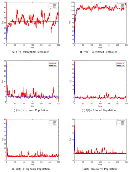
Now here, we give the discussion of the graphical representation and epidemiological feasibility of the proposed problem (2). For this, we use the numerical parameters values of Table 2 (${\mathbb{S}}_1$). The initial values for all the agents are also written Table 2 (${\mathbb{S}}_1$). Using Theorem 2 gives the conditions for vanishing the epidemic. Few of the achievements are obtained from the analysis of stability in the stochastically investigated model. Theorem 2 is satisfied if the reproduction value is ${\mathbf{R}}_0<1$. This shows that the epidemic vanishing probability will be one in the stochastic model. Similarly, if ${\mathfrak{R}}_0^D<1$, the idealistic problem (2) will be asymptotic and globally stable. For both curves, they converge to the free critical value. This is given in Figure 1, which implies that COVID-19 infection will die out of society, given some important conditions.The simulations of all the agents are provided in Figure 1a–e.

Table 2. Parameter values used in the simulation of model (2).

Parameters	${\mathbb{S}}_1$	${\mathbb{S}}_2$	Source
$\mathrm{\Pi }$	1.50	3.50	assumed
$\tau$	0.02	0.30	assumed
$\eta$	0.07	0.03	assumed
$\delta$	0.01	0.03	assumed
$\sigma$	0.01	0.05	assumed
$\kappa$	0.02	0.04	assumed
${\rho }_1$	0.05	0.10	assumed
${\rho }_2$	0.35	0.20	assumed
${\rho }_3$	0.05	0.30	assumed
${\mu }_1$	0.55	0.40	assumed
${\mu }_2$	0.15	0.50	assumed
$\mathbb{S}\left(0\right)$	50.0	4.00	assumed
$\mathbb{V}\left(0\right)$	20.0	3.00	assumed
$\mathbb{E}\left(0\right)$	30.0	1.00	assumed
$\mathbb{I}\left(0\right)$	40.0	2.00	assumed
$\mathbb{H}\left(0\right)$	40.0	2.00	assumed
$\mathbb{R}\left(0\right)$	10.0	1.00	assumed
${\mathrm{\Phi }}_1$	1.25	1.20	assumed
${\mathrm{\Phi }}_2$	1.23	1.25	assumed
${\mathrm{\Phi }}_3$	1.35	1.15	assumed
${\mathrm{\Phi }}_4$	1.20	1.05	assumed
${\mathrm{\Phi }}_5$	1.15	1.22	assumed
${\mathrm{\Phi }}_6$	1.10	1.15	assumed

Figure 1. Solution paths of the model (2) when the numerical values are taken as shown in the 2nd column of Table 2.

Next, we provide the digital findings for the stationary points of distributions. In Lemma 3, an ergodic condition is used to prove that the system is more realistic in the stochastic approach and has one stationary distribution. The stochastically given problem (2) is proposed for the parameter values given in Table 2 $\left({\mathbb{S}}_2\right)$ and evaluated as ${\mathbb{R}}_0^s>1$, so using Theorem 3, which is fulfilled, because of small intensities of white noises, the infection reflection will lie. We observe in Figure 2 that the infected system (2) will lie or remain in the mean, which may validate the output of Theorem 3 which implies that the system (2) lies on ergodic stationary distributions. The Susceptible, Vaccinated, Expose, Infected, and Recovered individual stationary distribution numerical simulations can be clearly seen in Figure 2a–f, respectively. Theorem 3 implies that model (2) must be ergodic stationary distributions. Figure 3 confirms this.

Figure 2. Solutions paths of the model (2) when the numerical values are taken as shown in the third column of Table 2.

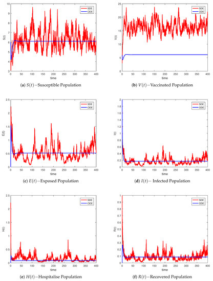
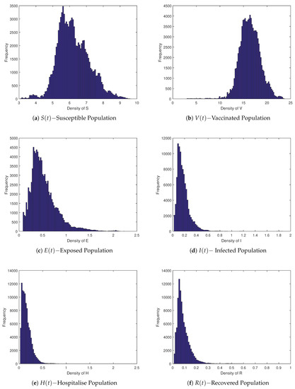
Figure 3. Ergodic stationary distribution of model (2).

8. Conclusions

In this article, we discussed the asymptotic dynamics of a stochastic COVID-19 epidemic model with a general incident rate and the effect of vaccination. Firstly, we analyzed the considered model for the unique globally non-negative root along with an initial approximation. The stability of the solution of the given model was also computed by the help of the Lyapunov operator. For eliminating the infection from society, we derived the reproduction value ${\mathbf{R}}_{\mathbf{0}}<1$. The Lyapunov function method proved that an ergodic stationary division for the non-negative root of the given system exists and is unique, which shows that for ${\mathbb{R}}_0^s>1$, the disease may lie in the community. Few of the numerical simulations have been performed by the $RK4$ approach for the validation of the obtained results. We also will study in our future research work the effect of Levy noises on the dynamics of a more complex population system.

References

- Huang, C.; Wang, Y.; Li, X.; Ren, L.; Zhao, J.; Hu, Y.; Zhang, L. Clinical features of patients infected with 2019 novel coronavirus in Wuhan, China. Lancet 2020, 395, 497–506. [Google Scholar] [CrossRef] [PubMed]
- Ding, Y.; Jiao, J.; Zhang, Q.; Zhang, Y.; Ren, X. Stationary Distribution and Extinction in a Stochastic SIQR Epidemic Model Incorporating Media Coverage and Markovian Switching. Symmetry 2021, 13, 1122. [Google Scholar] [CrossRef]
- Atangana, A. Modelling the spread of COVID-19 with new fractal-fractional operators: Can the lockdown save mankind before vaccination? Chaos Solitons Fractals 2020, 136, 109860. [Google Scholar] [CrossRef] [PubMed]
- Tul, A.Q.; Anjum, N.; Zeb, A.; Djilali, S.; Khan, Z.A. On the analysis of Caputo fractional order dynamics of Middle East Lungs Coronavirus (MERS-CoV) model. Alex. Eng. J. 2022, 61, 5123–5131. [Google Scholar]
- Ali, I.; Khan, S.U. Threshold of Stochastic SIRS Epidemic Model from Infectious to Susceptible Class with Saturated Incidence Rate Using Spectral Method. Symmetry 2022, 14, 1838. [Google Scholar] [CrossRef]
- Anwarud, D.; Li, Y.; Shah, M.A. The complex dynamics of hepatitis B infected individuals with optimal control. J. Syst. Sci. Complex. 2021, 34, 1301–1323. [Google Scholar]
- Allen, L.J.S. An introduction to stochastic epidemic models. In Mathematical Epidemiology; Springer: Berlin/Heidelberg, Germany, 2008; pp. 81–130. [Google Scholar]
- Lei, Q.; Yang, Z. Dynamical behaviours of a stochastic SIRI epidemic model. Appl. Anal. 2016, 96, 1–13. [Google Scholar]
- Özdemir, N.; Agrawal, O.P.; Karadeniz, D.; İskender, B.B. Fractional optimal control problem of an axis-symmetric diffusion-wave propagation. Phys. Scr. 2009, T136, 014024. [Google Scholar] [CrossRef]
- Din, A.; Yassine, S. Long-term bifurcation and stochastic optimal control of a triple-delayed Ebola illness model with vaccination and quarantine strategies. Fractal Fract. 2022, 6, 578. [Google Scholar] [CrossRef]
- Khan, A.; Yassine, S. Stochastic modeling of the Monkeypox 2022 epidemic with cross-infection hypothesis in a highly disturbed environment. Math. Biosci. Eng. 2022, 19, 13560–13581. [Google Scholar] [CrossRef] [PubMed]
- Din, A.; Li, Y.; Tahir, K.; Gul, Z. Mathematical analysis of spread and control of the novel corona virus (COVID-19) in China. Chaos Solitons Fractals 2020, 141, 110286. [Google Scholar] [CrossRef] [PubMed]
- Din, A.; Li, Y.; Abdullahi, Y. Delayed hepatitis B epidemic model with stochastic analysis. Chaos Solitons Fractals 2021, 146, 110839. [Google Scholar] [CrossRef]
- Yassine, S.; Khan, A.; Din, A.; Kiouach, D.; Rajasekar, S.P. Determining the global threshold of an epidemic model with general interference function and high-order perturbation. AIMS Math. 2022, 7, 19865–19890. [Google Scholar]
- Alzahrani, E.O.; Khan, M.A. Modeling the dynamics of Hepatitis E with optimal control. Chaos Solitons Fractals 2018, 116, 287–301. [Google Scholar] [CrossRef]
- Olver, P.J. Applications of Lie Groups to Differential Equations; Springer: Berlin/Heidelberg, Germany, 2000. [Google Scholar]
- Olver, P.J. Equivalence, Invariants, and Symmetry; Cambridge University Press: Cambridge, UK, 1995. [Google Scholar]
- Zhang, T.; Ding, T.; Gao, N.; Song, Y. Dynamical behavior of a stochastic SIRC model for influenza A. Symmetry 2020, 12, 745. [Google Scholar] [CrossRef]
- Gaeta, G.; Rodriguez-Quintero, N. Lie-point symmetries and stochastic differential equations. J. Phys. A Math. Gen. 1999, 32, 8485–8505. [Google Scholar] [CrossRef]
- Gaeta, G. Lie-point symmetries and stochastic differential equations: II. J. Phys. A Math. Gen. 2000, 33, 4883–4902. [Google Scholar] [CrossRef]
- Zhang, X.-B.; Wang, X.-D.; Huo, H. Extinction and stationary distribution of a stochastic SIRS epidemic model with standard incidence rate and partial immunity. Phys. Stat. Mech. Appl. 2019, 531, 121548. [Google Scholar] [CrossRef]
- Din, A.; Saida, A.; Amina, A. A stochastically perturbed co-infection epidemic model for COVID-19 and hepatitis B virus. Nonlinear Dyn. 2022, 28, 1–25. [Google Scholar] [CrossRef] [PubMed]
- Khasminskii, R. Stochastic Stability of Differential Equations; Springer Science & Business Media: Berlin/Heidelberg, Germany, 2011; Volume 66. [Google Scholar]
Disclaimer/Publisher’s Note: The statements, opinions and data contained in all publications are solely those of the individual author(s) and contributor(s) and not of MDPI and/or the editor(s). MDPI and/or the editor(s) disclaim responsibility for any injury to people or property resulting from any ideas, methods, instructions or products referred to in the content. |
© 2023 by the authors. Licensee MDPI, Basel, Switzerland. This article is an open access article distributed under the terms and conditions of the Creative Commons Attribution (CC BY) license (https://creativecommons.org/licenses/by/4.0/).