A New More Flexible Class of Distributions on (0,1): Properties and Applications to Univariate Data and Quantile Regression

Abstract

In this paper, we will present a new, more flexible class of distributions with a domain in the interval (0,1), which presents heavier tails than other distributions in the same domain, such as the $Beta$, Kumaraswamy, and Weibull Unitary distributions. This new distribution is obtained as a transformation of two independent random variables with a Weibull distribution, which we will call the Generalized Unitary Weibull distribution. Considering a particular case, we will obtain an alternative to the $Beta$, Kumaraswamy, and Weibull Unitary distributions. We will call this new distribution of two parameters the type 2 unitary Weibull distribution. The probability density function, cumulative probability distribution, survival function, hazard rate, and some important properties that will allow us to infer are provided. We will carry out a simulation study using the maximum likelihood method and we will analyze the behavior of the parameter estimates. By way of illustration, real data will be used to show the flexibility of the new distribution by comparing it with other distributions that are known in the literature. Finally, we will show a quantile regression application, where it is shown how the proposed distribution fits better than other competing distributions for this type of application.

1. Introduction

There are various probability distributions with support on (0,1). One of the most used is the $Beta$ distribution, which is a family of continuous probability distributions defined in the interval (0,1) with two shape parameters, both positive, normally denoted by $\alpha$ and $\beta$.

In Bayesian inference, the $Beta$ distribution is generally used as the conjugate prior to probability distribution for the Bernoulli, binomial, negative binomial, and geometric distributions. For example, the $Beta$ distribution can be used in Bayesian analysis to describe any initial knowledge about the probability of success. In addition, it is a density that is usually used to model the data associated with percentages and proportions.

The usual formulation of the $Beta$ distribution is also known as the type I $Beta$ distribution, whose density function is provided by:

$$\begin{array}{c}\hfill f_X\left(x\right)=\frac{\Gamma (\alpha +\beta )}{\Gamma \left(\alpha \right)\Gamma \left(\beta \right)}{x}^{\alpha -1}{(1-x)}^{\beta -1},\end{array}$$

(1)

where $\alpha$, $\beta >0$ are shape parameters, with $0<x<1$. We denote this by writing $X\sim Beta(\alpha ,\beta )$.

A distribution similar to $Beta$ is the Kumaraswamy distribution [1], but it is simpler in the sense that simulations can be obtained from the inverse of the cumulative distribution, since it has a closed expression, alike the quantiles. Its density is defined by:

$$\begin{array}{c}\hfill f_X\left(x\right)=\alpha \beta x^{\alpha -1}{(1-x^{\alpha })}^{\beta -1},\end{array}$$

(2)

where $\alpha$, $\beta >0$ are the shape parameters, with $0<x<1$. We denote this by writing $X\sim KW(\alpha ,\beta )$.

Mazucheli et al. [2] show the Unitary Weibull distribution where they present some inferential procedures. Mazucheli et al. [3] present a unitary version of the Weibull distribution as an alternative to the $KW$ distribution to model quantiles conditional on covariates. The stochastic representation of a Unitary Weibull distribution is provided by $V=e^{-X}$, with $X\sim Weibull(\alpha ,\beta )$, denoted by $V\sim UW(\alpha ,\beta )$, which has a density function provided by:

$$\begin{array}{c}\hfill f_V\left(v\right)=\frac{1}{v}\alpha \beta {[-log\left(v\right)]}^{\beta -1}exp\left\{-\alpha {[-log\left(v\right)]}^{\beta }\right\},0<v<1.\end{array}$$

(3)

In this paper, the Generalized Unitary Weibull distribution of a random variable Y is presented based on a transformation of two independent random variables with distributions $Weibull({\theta }_1,\alpha )$ and $Weibull({\theta }_2,\beta )$, denoted by $Y\sim GUW({\theta }_1,{\theta }_2,\alpha ,\beta )$. In particular, we will study the case for ${\theta }_1={\theta }_2=\theta$ and $\alpha =1$ that we will call Weibull Unitary distribution type 2, denoted by $UW2(\theta ,\beta )$, where $\theta$, $\beta >0$.

The article is organized in the following manner. In Section 2, we provide the stochastic representation, the pdf of a random variable with $GUW$ distribution, and present some properties and the distribution $UW2$ as a particular case. The cumulative distribution function (cdf), quantiles, reliability functions, and hazard rate, moments, skewness coefficients, and kurtosis are also provided. Some statistical properties are provided. The Canonical Unitary Weibull distribution and its properties are presented. In Section 3, an inference is made through a simulation study of the parameter estimates using the maximum likelihood method. In addition, the $Beta$, $KW$, $UW$, and $UW2$ distributions are fitted to real data sets in Section 4. In Section 5, a discussion and the main conclusions are presented.

2. The Generalized Unitary Weibull Family of Distribution

A random variable Y has a Generalized Unitary Weibull distribution, of parameters ${\theta }_1$, ${\theta }_2$, $\alpha$, and $\beta >0$, denoted by $Y\sim GUW({\theta }_1,{\theta }_2,\alpha ,\beta )$, if its stochastic representation is provided by:

$$Y=\frac{X_1}{X_1+X_2},$$

(4)

where $X_1\sim Weibull({\theta }_1,\alpha )$ and $X_2\sim Weibull({\theta }_2,\beta )$, $X_1$, and $X_2$ are independent random variables. Its density function is presented below.

2.1. Density Function

Proposition 1.

Let $Y\sim GUW({\theta }_1,{\theta }_2,\alpha ,\beta )$ then the density function of Y is:

$$\begin{array}{ccc}\hfill f_Y\left(y\right)& =& \frac{{\theta }_1{\theta }_2{y}^{{\theta }_1-1}}{{\beta }^{{\theta }_2}{\alpha }^{{\theta }_1}{(1-y)}^{{\theta }_1+1}}{\int }_0^{\infty }{w}^{{\theta }_1+{\theta }_2-1}exp\left\{-\left[{\left(\frac{yw}{\alpha (1-y)}\right)}^{{\theta }_1}+{\left(\frac{w}{\beta }\right)}^{{\theta }_2}\right]\right\}dw\hfill \end{array}$$

(5)

where $0<y<1$, ${\theta }_1$, ${\theta }_2$, α, and $\beta >0$.

Proof. 

Using the stochastic representation provided in (4), we have that:

$$\begin{array}{ccc}\hfill X_1\sim Weibull({\theta }_1,\alpha )& \Rightarrow & f_{X_1}\left(x\right)=\frac{{\theta }_1}{\alpha }{\left(\frac{x}{\alpha }\right)}^{{\theta }_1-1}exp\left\{-{\left(\frac{x}{\alpha }\right)}^{{\theta }_1}\right\},x>0,\hfill \end{array}$$

(6)

$$\begin{array}{ccc}\hfill X_2\sim Weibull({\theta }_2,\beta )& \Rightarrow & f_{X_2}\left(x\right)=\frac{{\theta }_2}{\beta }{\left(\frac{x}{\beta }\right)}^{{\theta }_2-1}exp\left\{-{\left(\frac{x}{\beta }\right)}^{{\theta }_2}\right\},x>0,\hfill \end{array}$$

(7)

are independent random variables and, using the Jacobian of the transformation, it follows that:

$$\begin{array}{c}\hfill \left.\begin{array}{c}y=\frac{x_1}{x_1+x_2}\hfill \\ w=x_2\hfill \end{array}\right\}\Rightarrow \left.\begin{array}{c}{x}_1=\frac{yw}{1-y}\hfill \\ x_2=w\hfill \end{array}\right\}\Rightarrow J=\left|\begin{array}{cc}\frac{\partial x_1}{\partial y}\hfill & \frac{\partial x_1}{\partial w}\hfill \\ \frac{\partial x_2}{\partial y}\hfill & \frac{\partial x_2}{\partial w}\hfill \end{array}\right|=\left|\begin{array}{cc}\frac{w}{{(1-y)}^2}\hfill & \frac{y}{1-y}\hfill \\ 0\hfill & 1\hfill \end{array}\right|=\frac{w}{{(1-y)}^2}.\end{array}$$

(8)

Hence,

$$\begin{array}{ccc}\hfill f_{Y,W}(y,w)& =& \left|J\right|f_{X_1,X_2}\left(\frac{yw}{1-y},w\right)\hfill \\ & =& \frac{w}{{(1-y)}^2}{f}_{X_1}\left(\frac{yw}{1-y}\right)f_{X_2}\left(w\right)\hfill \\ & =& \frac{{\theta }_1{\theta }_2{y}^{{\theta }_1-1}{w}^{{\theta }_1+{\theta }_2-1}}{{\beta }^{{\theta }_2}{\alpha }^{{\theta }_1}{(1-y)}^{{\theta }_1+1}}exp\left\{-\left[{\left(\frac{yw}{\alpha (1-y)}\right)}^{{\theta }_1}+{\left(\frac{w}{\beta }\right)}^{{\theta }_2}\right]\right\},0<y<1,w>0.\hfill \end{array}$$

(9)

Therefore,

$$\begin{array}{ccc}\hfill f_Y\left(y\right)& =& \frac{{\theta }_1{\theta }_2{y}^{{\theta }_1-1}}{{\beta }^{{\theta }_2}{\alpha }^{{\theta }_1}{(1-y)}^{{\theta }_1+1}}{\int }_0^{\infty }{w}^{{\theta }_1+{\theta }_2-1}exp\left\{-\left[{\left(\frac{yw}{\alpha (1-y)}\right)}^{{\theta }_1}+{\left(\frac{w}{\beta }\right)}^{{\theta }_2}\right]\right\}dw,\hfill \end{array}$$

(10)

where $0<y<1$. □

Now, we provide some elementary properties.

Proposition 2.

Let $Y\sim GUW({\theta }_1,{\theta }_2,\alpha ,\beta )$ then:

1.

If ${\theta }_1={\theta }_2=\alpha =\beta =1$ then $Y\sim U(0,1)$, where U denotes the uniform distribution in (0,1).

2.

If ${\theta }_1={\theta }_2=\theta$, and $\alpha =\beta =1$ then $f_Y$ is symmetric.

3.

If ${\theta }_1={\theta }_2=\alpha =1$ then $f_Y\left(y\right)=\frac{\beta }{{[1+(\beta -1)y]}^2}$.

Proof. 

Let $Y\sim GUW({\theta }_1,{\theta }_2,\alpha ,\beta )$, whose density is represented in proposition 1.

1.

The result is obtained by replacing ${\theta }_1={\theta }_2=\alpha =\beta =1$ in the distribution of Y then $Y\sim U(0,1)$.

2.

If ${\theta }_1={\theta }_2=\theta$ and $\alpha =\beta =1$ then:

$$\begin{array}{ccc}\hfill f_Y\left(y\right)& =& \frac{\theta y^{\theta -1}{(1-y)}^{\theta -1}}{{[y^{\theta }+{(1-y)}^{\theta }]}^2},0<y<1.\hfill \end{array}$$

(11)

Then $f_Y\left(y\right)=f_Y(1-y)$.

3.

The result follows from plugging ${\theta }_1={\theta }_2=\alpha =1$ into the distribution of Y.

□

2.2. Density Function of the Unitary Weibull Distribution Type 2

Definition 1.

Setting ${\theta }_1={\theta }_2=\theta$ and $\alpha =1$ in (5), the density function of Y is provided for:

$$\begin{array}{c}\hfill f_Y\left(y\right)=\frac{\theta {\beta }^{\theta }{y}^{\theta -1}{(1-y)}^{\theta -1}}{[{\left(\beta y\right)}^{\theta }+{\left[{(1-y)}^{\theta }\right]}^2},0<y<1,\end{array}$$

(12)

which we will call Weibull Unitary distribution type 2, denoted by $Y\sim UW2(\theta ,\beta )$.

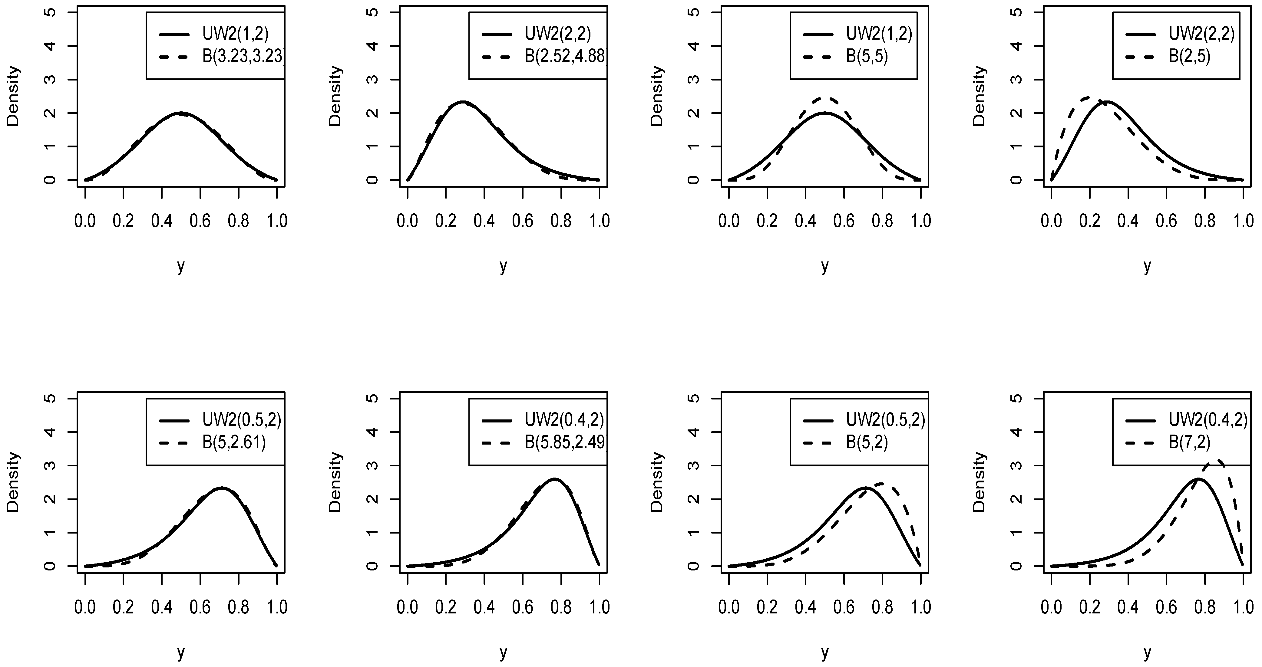
Figure 1 below show each pdf of the $UW2$ distribution compared to the $Beta$ distribution. It shows that, for certain values of the parameters, respectively, the distributions are very similar and in others there is quite a difference.

Figure 1. $UW2$ pdf for $\theta =2$ and different values of $\beta$.

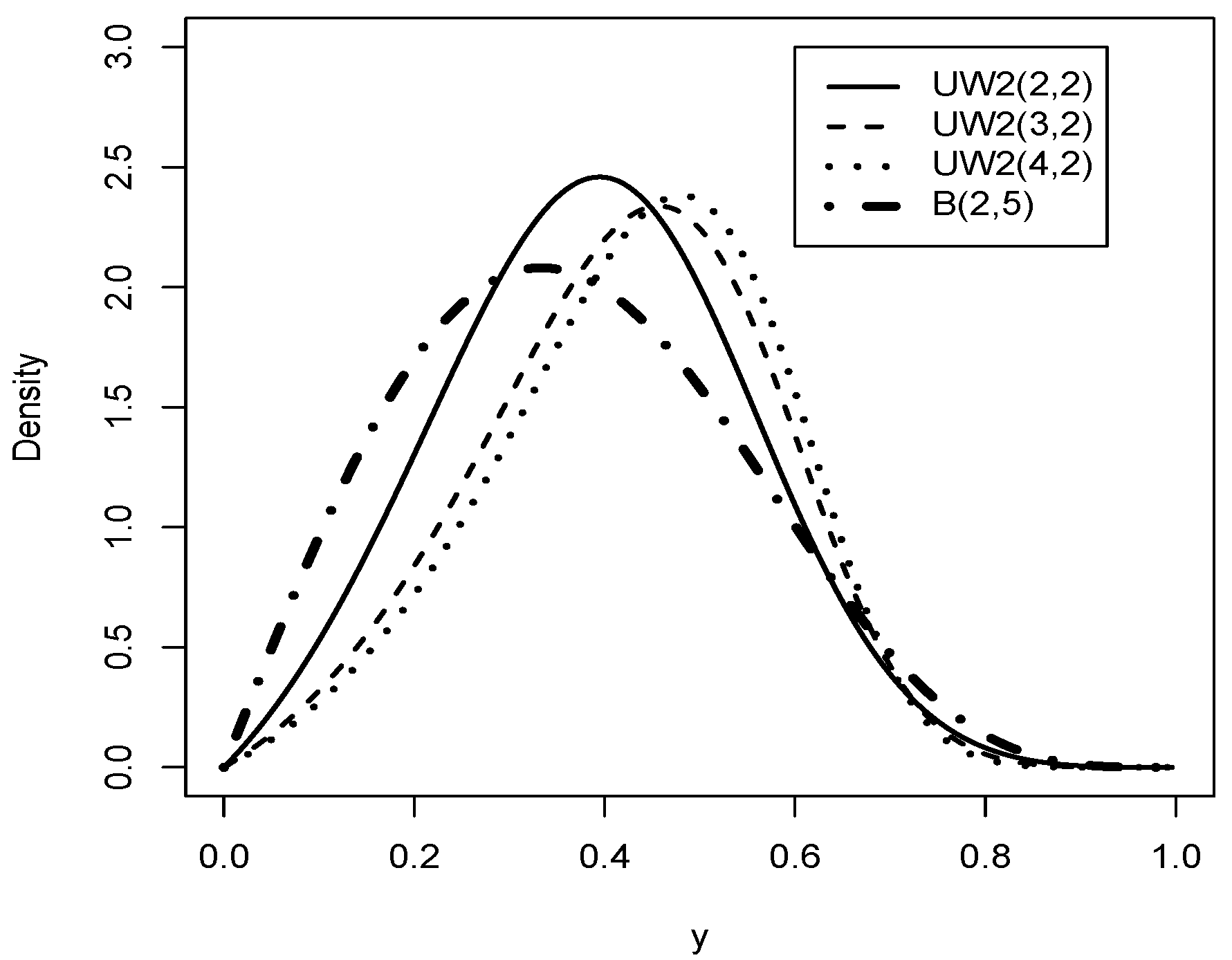
Figure 2 shows the pdfs of the $UW2$ distribution for $\beta =2$ and different values of $\theta$.

Figure 2. $UW2$ pdf for $\beta =2$ and different values of $\theta$.

Proposition 3.

Let $Y\sim UW2(\theta ,\beta )$. Then, the cdf of Y is provided by:

$$\begin{array}{ccc}\hfill F_Y\left(t\right)& =& {\left[1+{\left(\frac{1-t}{\beta t}\right)}^{\theta }\right]}^{-1},0<t<1.\hfill \end{array}$$

(13)

Proof. 

$$\begin{array}{ccc}\hfill F_Y\left(t\right)& =& {\int }_0^t{f}_Y\left(y\right)dy\hfill \\ & =& {\int }_0^t\frac{\theta {\beta }^{\theta }{y}^{\theta -1}{(1-y)}^{\theta -1}}{{[{\left(\beta y\right)}^{\theta }+{(1-y)}^{\theta }]}^2}dy\hfill \\ & =& \theta \beta {\int }_0^t\frac{{\left(\beta y\right)}^{\theta -1}{(1-y)}^{\theta -1}}{{\left(\beta y\right)}^{2\theta }{\left[1+{\left(\frac{1-y}{\beta y}\right)}^{\theta }\right]}^2}dy\hfill \\ & =& \theta \beta {\int }_0^t\frac{{\left(\frac{1-y}{\beta y}\right)}^{\theta -1}}{{\left(\beta y\right)}^2{\left[1+{\left(\frac{1-y}{\beta y}\right)}^{\theta }\right]}^2}dy.\hfill \end{array}$$

Performing the change of variable $u=\frac{1-y}{\beta y}$ y expanding the integral, we obtain the result. □

Corollary 1.

Let $Y\sim UW2(\theta ,\beta )$, then the quantile function of Y is provided by:

$$t={\left[1+\beta {\left(\frac{1}{p}-1\right)}^{\frac{1}{\theta }}\right]}^{-1},0<p<1.$$

(14)

Proof. 

Solving t from $p=F_Y\left(t\right)$ provides the result. □

In Figure 3, we graphically illustrate the behavior of the Cumulative distribution function of the $UW2$ distribution for different values of $\theta$ and $\beta =2$.

Figure 3. Cdf of $UW2$ for different values $\theta$ and $\beta =2$.

2.3. The Reliability, Hazard Rate Functions and Increasing Failure Rate

Two important measures of reliability are the reliability function and hazard (failure) rate function. The reliability function of a random variable Y is defined by $S_Y\left(t\right)=1-F_Y\left(t\right)$, where $F_Y$ denotes the cdf of Y. The risk rate function is defined by $h_Y\left(t\right)=f_Y\left(t\right)/(1-F_Y\left(t\right))$. For the distribution $UW2$, as a direct consequence of Proposition 3, both reliability measures can be expressed in closed form. The corresponding expression is obtained in the following Proposition simple form.

In Table 1, it can be seen that the $UW2$ distribution better captures the values’ outliers compared to the $UW$, $KW$, and $\beta$ distributions, since the reliability is higher.

Table 1. Reliability function comparisond for distributions of $UW2$, $UW$, $KW$, and $\beta$.

	${\mathit{S}}_{\mathit{Y}}\left(\mathit{t}\right)=\mathit{P}(\mathit{Y}>\mathit{t})$
$\mathit{t}$	$\mathit{UW}\mathbf{2}(\mathbf{1},\mathbf{5})$	$\mathit{UW}(\mathbf{1},\mathbf{5})$	$\mathit{KW}(\mathbf{1},\mathbf{5})$	$\mathit{Beta}(\mathbf{1},\mathbf{5})$
0.70	0.0789474	0.0057559	0.0024300	0.0024300
0.75	0.0625000	0.0019685	0.0009766	0.0009766
0.80	0.0476191	0.0005531	0.0003200	0.0003200
0.85	0.0340909	0.0001134	0.0000759	0.0000759
0.90	0.0217391	0.0000130	0.0000100	0.0000100
0.95	0.0104167	0.0000004	0.0000003	0.0000003

Proposition 4.

Let $Y\sim UW2(\theta ,\beta )$. Then, the hazard rate funtion of Y is provided by:

$$\begin{array}{ccc}\hfill h\left(t\right)& =& \frac{\theta {\beta }^{\theta }{t}^{\theta -1}}{(1-t)[{\left(\beta t\right)}^{\theta }+{(1-t)}^{\theta }]}.\hfill \end{array}$$

(15)

Proof. 

$$\begin{array}{ccc}\hfill h_Y\left(t\right)& =& f_Y\left(t\right)/(1-F_Y\left(t\right)).\hfill \end{array}$$

(16)

Replacing $f_Y\left(t\right)$ and $F_Y\left(t\right)$ provides the result. □

Figure 4 shows the hazard rate function of the $UW2$ distribution for different values of $\theta$ and $\beta =2$. Looking at the graphical representation, it is clear that it presents a wide variety of forms. Therefore, the new family of distributions is flexible enough to model real data sets.

Figure 4. The hazard rate functions for the $UW2$ distribution.

Next, we present the Increasing Failure Rate, which is defined as the derivative of the failure rate function provided in (15).

Proposition 5.

Let Y have distribution $UW2(\theta ,\beta )$. Then for any θ and $\beta >0$ the random variable Y has Increasing Failure Rate (IFR).

Proof. 

The first derivative of h provided in (15) can be written as follows

$$\begin{array}{ccc}\hfill h^{\prime }\left(t\right)& =& \frac{{\beta }^{\theta }\theta t^{\theta -2}\left(\theta {\left(1-t\right)}^{\theta }+2t{\left(1-t\right)}^{\theta }-{\left(\beta t\right)}^{\theta }+2t{\left(\beta t\right)}^{\theta }-{\left(1-t\right)}^{\theta }\right)}{{\left({\left(\beta t\right)}^{\theta }+{\left(1-t\right)}^{\theta }\right)}^2{\left(1-t\right)}^2}.\hfill \end{array}$$

(17)

It is clear that $h^{\prime }(t;\theta ,\beta )>0$ since $t>0$, $\beta >0$ and $\theta >0$, which implies the result. □

2.4. Moments

The following statement shows the moments for the $UW2$ distribution. Essentially, these moments are expressed as a numerical integral (the problem of obtaining a closed analytic expression remains open).

Definition 2.

Let $Y\sim UW2(\theta ,\beta )$. Hence, for $r=1,2,3,\dots$ we define:

$${\mu }_r(\theta ,\beta )=E\left(Y^r;\theta ,\beta \right)=\theta {\beta }^{\theta }{\int }_0^1\frac{y^{r+\theta -1}{(1-y)}^{\theta -1}}{{[{\left(\beta y\right)}^{\theta }+{(1-y)}^{\theta }]}^2}dy.$$

(18)

Proposition 6.

Let $Y\sim UW2(\theta ,\beta )$ then:

$$\begin{array}{ccc}\hfill E(Y^r;\theta ,\beta )& =& E\left({(1-Y)}^r;\theta ,\frac{1}{\beta }\right).\hfill \end{array}$$

(19)

Proof. 

$$\begin{array}{ccc}\hfill E\left(Y^r;\theta ,\beta \right)& =& \theta {\beta }^{\theta }{\int }_0^1\frac{y^{\theta +r-1}{(1-y)}^{\theta -1}}{{[{\left(\beta y\right)}^{\theta }+{(1-y)}^{\theta }]}^2}dy\hfill \\ & =& \theta {\left(\frac{1}{\beta }\right)}^{\theta }{\int }_0^1\frac{{(1-y)}^{\theta +r-1}{y}^{\theta -1}}{{[y^{\theta }+{\left(\frac{(1-y)}{\beta }\right)}^{\theta }]}^2}dy\hfill \\ & =& E\left({(1-Y)}^r;\theta ,\frac{1}{\beta }\right)\hfill \end{array}$$

□

In particular, for $r=1$ we have:

$$\begin{array}{ccc}\hfill {\mu }_1(\theta ,\beta )& =& 1-{\mu }_1\left(\theta ,\frac{1}{\beta }\right).\hfill \end{array}$$

(20)

Remark 1.

This Proposition allows us to reaffirm that, for $\beta =1$ and any value of the parameter θ, the density $UW2$ is symmetric (case $r=1$).

Remark 2.

From definition 2, the skewness and kurtosis coefficients can be obtained through:

$${\beta }_1=\frac{{\mu }_3-3{\mu }_2{\mu }_1+2{\mu }_1^3}{{\left[({\mu }_2-{\mu }_1^2)\right]}^{3/2}}$$

(21)

and

$${\beta }_2=\frac{{\mu }_4-4{\mu }_1{\mu }_3+6{\mu }_1^2{\mu }_2-3{\mu }_1^4}{{({\mu }_2-{\mu }_1^2)}^2},$$

(22)

respectively, which do not present a closed expression, so they must be obtained using numerical methods.

Corollary 2.

Let $Y\sim UW2(\theta ,\beta )$, then:

$$\begin{array}{ccc}\hfill {\beta }_1(\theta ,\beta )& =& -{\beta }_1\left(\theta ,\frac{1}{\beta }\right)\hfill \end{array}$$

(23)

$$\begin{array}{ccc}\hfill {\beta }_2(\theta ,\beta )& =& {\beta }_2\left(\theta ,\frac{1}{\beta }\right).\hfill \end{array}$$

(24)

Proof. 

Using Proposition 6 for $r=1,2,3,4$ and substituting in (21) and (22), respectively, the required result is obtained. □

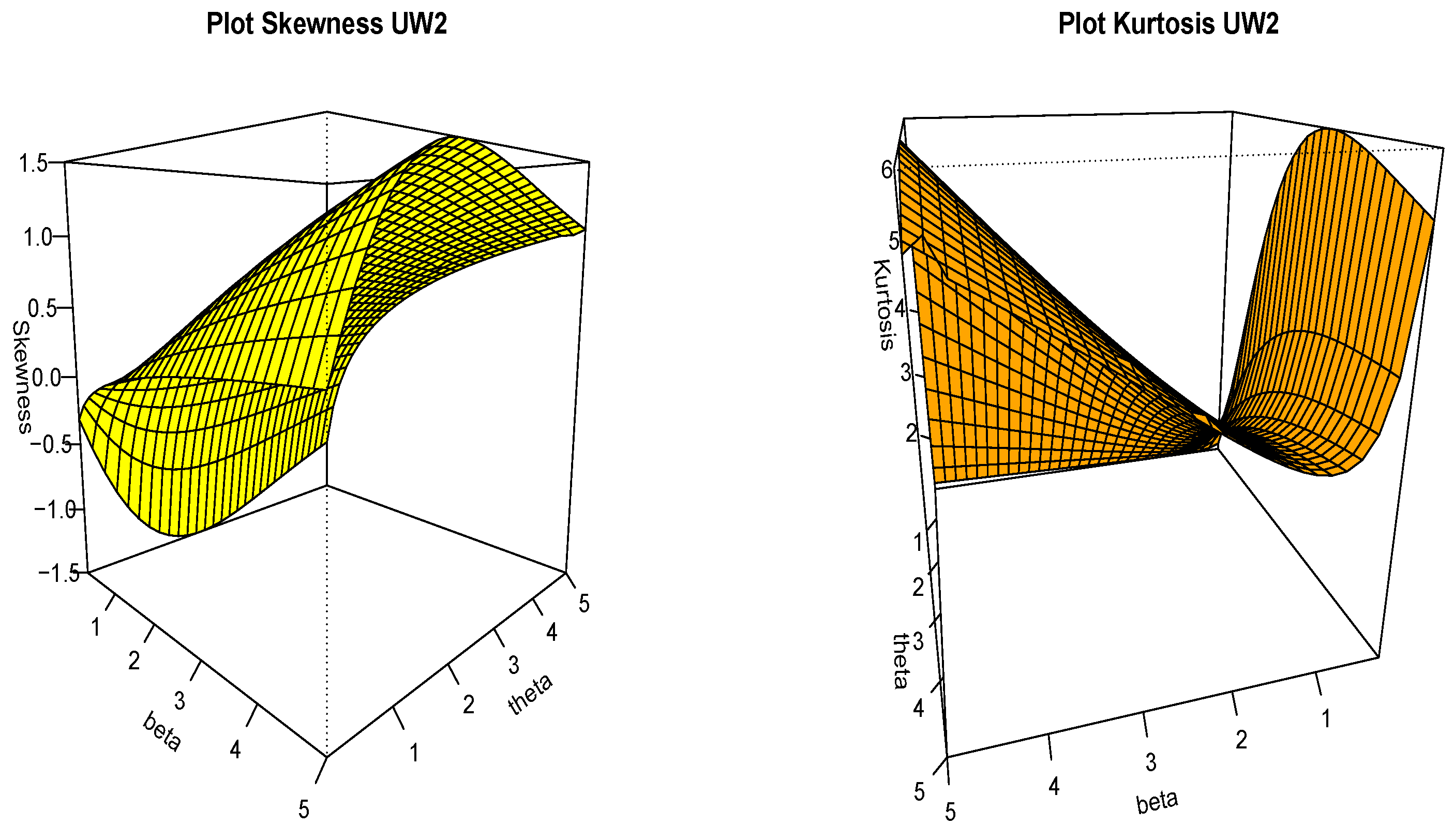
Figure 5 and Table 2 graphically and numerically show the behavior of the asymmetry and kurtosis coefficients of the $UW2$ distribution and are consistent with what is represented in corollary 2. That is, the value of the asymmetry coefficient, given a value of the parameter $\theta$, is the same for $\beta$ as for $1/\beta$, but with the opposite sign. For example: ${\beta }_1(5,1/2)=-0.4592$ and ${\beta }_1(5,2)=0.4592$. Similarly, the value of the kurtosis coefficient, given a value of the parameter $\theta$, is the same for $\beta$ as it is for $1/\beta$. For example: ${\beta }_2(5,1/2)={\beta }_2(5,2)=4.6954$.

Figure 5. Plots of the skewness (left) and kurtosis of the $UW2$ distribution (right).

Table 2. Skewness and kurtosis values of the $UW2$ model with different values of $\theta$ and $\beta$.

	$\mathit{Skewness}$					$\mathit{Kurtosis}$
$\mathbf{\theta }$	$\mathbf{\beta }=\mathbf{1}/\mathbf{2}$	$\mathbf{\beta }=\mathbf{1}/\mathbf{3}$	$\mathbf{\beta }=\mathbf{1}$	$\mathbf{\beta }=\mathbf{2}$	$\mathbf{\beta }=\mathbf{3}$	$\mathbf{\beta }=\mathbf{1}/\mathbf{2}$	$\mathbf{\beta }=\mathbf{1}/\mathbf{3}$	$\mathbf{\beta }=\mathbf{1}$	$\mathbf{\beta }=\mathbf{2}$	$\mathbf{\beta }=\mathbf{3}$
1	−0.4861	−0.7849	0	0.4861	0.7849	2.0928	2.5644	1.8000	2.0928	2.5644
2	−0.5980	−0.9739	0	0.5980	0.9739	3.0459	3.9578	2.5013	3.0459	3.9578
3	−0.5744	−0.9279	0	0.5744	0.9279	3.5809	4.5497	2.9939	3.5809	4.5497
4	−0.5176	−0.8255	0	0.5176	0.8255	3.8564	4.7050	3.3240	3.8564	4.7050
5	−0.4592	−0.7237	0	0.4592	0.7237	3.9995	4.6954	3.5460	3.9994	4.6954
6	−0.4077	−0.6363	0	0.4077	0.6363	4.0765	4.6377	3.6984	4.0765	4.6377
7	−0.3642	−0.5641	0	0.3642	0.5641	4.1201	4.5736	3.8058	4.1201	4.5736
8	−0.3278	−0.5048	0	0.3278	0.5048	4.1460	4.5161	3.8836	4.1460	4.5161
9	−0.2972	−0.4557	0	0.2972	0.4557	4.1620	4.4678	3.9412	4.1620	4.4678
10	−0.2715	−0.4148	0	0.2715	0.4148	4.1723	4.4281	3.9848	4.1723	4.4281
11	−0.2496	−0.3802	0	0.2496	0.3802	4.1793	4.3957	4.0186	4.1793	4.3957
12	−0.2307	−0.3508	0	0.2307	0.3508	4.1840	4.3692	4.0472	4.1840	4.3693
13	−0.2144	−0.3254	0	0.2144	0.3254	4.1874	4.3475	4.0665	4.1874	4.3475
14	−0.2002	−0.3033	0	0.2002	0.3033	4.1899	4.3295	4.0765	4.1899	4.3295
15	−0.1877	−0.2840	0	0.1877	0.2840	4.1917	4.3144	4.0979	4.1917	4.3145
16	−0.1766	−0.2670	0	0.1766	0.2670	4.1932	4.3018	4.1096	4.1931	4.3018
17	−0.1667	−0.2518	0	0.1667	0.2518	4.1942	4.2911	4.1194	4.1942	4.2908
18	−0.1578	−0.2393	0	0.1578	0.2382	4.1951	4.4034	4.1278	4.1951	4.2837
19	−0.1498	−0.2261	0	0.1498	0.2263	4.1958	4.2741	4.1350	4.1958	4.2692
20	−0.1426	−0.2405	0	0.1426	0.2149	4.1963	5.7680	4.1411	4.1963	4.2746

2.5. Some Statistical Properties

2.5.1. Entropy of $UW2$

The entropy $H(\Theta )$ can be obtained using the density function of Y; specifically, the following form expression is obtained:

$$\begin{array}{c}\hfill H(\Theta )=-{\int }_0^1{f}_Y(y,\Theta )ln\left(f_Y(y,\Theta )\right)dy.\end{array}$$

(25)

If Y be a random variable with $\mathrm{UW}2(Y;\theta ,\beta )$ distribution. So, the entropy of Y is provided by:

$$\begin{array}{c}\hfill H(\theta ,\beta )=-{\int }_0^1\frac{\theta {\beta }^{\theta }{y}^{\theta }{(1-y)}^{\theta -1}}{{\left({\left(\beta y\right)}^{\theta }+{\left(1-y\right)}^{\theta }\right)}^2}ln\left(\frac{\theta {\beta }^{\theta }{y}^{\theta }{(1-y)}^{\theta -1}}{{\left({\left(\beta y\right)}^{\theta }+{\left(1-y\right)}^{\theta }\right)}^2}\right)dy.\end{array}$$

(26)

Table 3 shows the entropy values of the $UW2$ distribution for different values of the parameters $\theta$ and $\beta$.

Table 3. Entropy values for the distribution $UW2$($\theta ,\beta$) for different values of $\theta$ and $\beta$.

$\mathit{\theta }$	$\mathit{\beta }=1/3$	$\mathit{\beta }=1/2$	$\mathit{\beta }=1$	$\mathit{\beta }=2$	$\mathit{\beta }=3$
1	−0.1976	−0.0798	0.0000	−0.0781	−0.1939
2	−0.5145	−0.3657	−0.2640	−0.3657	−0.5146
3	−0.8398	−0.6808	−0.5714	−0.6808	−0.8398
4	−1.0984	−0.9350	−0.8223	−0.9350	−1.0984
5	−1.3079	−1.1423	−1.0279	−1.1423	−1.3079
6	−1.4828	−1.3159	−1.2006	−1.3159	−1.4828
7	−1.6324	−1.4648	−1.3488	−1.4648	−1.6324
8	−1.7630	−1.5949	−1.4785	−1.5949	−1.7630
9	−1.8788	−1.7103	−1.5936	−1.7103	−1.8788
10	−1.9827	−1.8139	−1.6971	−1.8139	−1.9827
11	−2.0770	−1.9080	−1.7910	−1.9080	−2.0770
12	−2.1632	−1.9940	−1.8769	−1.9940	−2.1632
13	−2.2426	−2.0733	−1.9561	−2.0733	−2.2426
14	−2.3162	−2.1469	−2.0295	−2.1469	−2.3162
15	−2.3848	−2.2154	−2.0980	−2.2154	−2.3848
16	−2.4490	−2.2795	−2.1621	−2.2795	−2.4490
17	−2.5093	−2.3398	−2.2223	−2.3398	−2.5093
18	−2.5663	−2.3967	−2.2792	−2.3967	−2.5663
19	−2.6201	−2.4505	−2.3330	−2.4505	−2.6201
20	−2.6713	−2.5016	−2.3841	−2.5016	−2.6713

2.5.2. Mean Residual Life

An important reliability quantity for positive random variables is the mean residual life, which is defined as $\mu (t;\theta ,\beta )=\frac{1}{1-F_Y\left(t\right)}{\int }_t^{\infty }(1-F_Y\left(y\right))dy,$$t>0$.

For the case that $Y\sim UW2(\theta ,\beta )$, then the mean residual life of Y is obtained by replacing:

$$\begin{array}{ccc}\hfill F_Y\left(t\right)& =& {\left(1+{\left(\frac{1-y}{\beta y}\right)}^{\theta }\right)}^{-1},t>0.\hfill \end{array}$$

(27)

2.5.3. Incomplete Moments

The r-th incomplete moment of $Y\sim f(y;\Theta )$ is defined as:

$$\begin{array}{ccc}\hfill m_r(y;\Theta )& =& {\int }_0^y{t}^{r}f(t;\Theta )dt.\hfill \end{array}$$

(28)

If $Y\sim UW2(\theta ,\beta )$, then the r-th incomplete moment of Y is provided by:

$$m_r(y;\theta ,\beta )={\int }_0^y\frac{t^{\theta +r-1}{(1-t)}^{\theta -1}}{{[{\left(\beta t\right)}^{\theta }+{(1-t)}^{\theta }]}^2}dt,0<y<1.$$

(29)

An interesting application of the first incomplete moment is that the mean deviation about the mean $\mu$ of Y can be directly obtained, specifically by means of the relation (see [4]):

$$\begin{array}{ccc}\hfill E\left(|Y-\mu |\right)& =& 2\mu F(\mu ;\theta ,\beta )-2m_1(\mu ;\theta ,\beta ),\hfill \end{array}$$

(30)

where $\mu =E\left[Y\right]$.

2.5.4. Lorenz Curve and the Gini Index

The Lorentz curve and Gini coefficient are tools used in the field of economics to measure income inequality in a society.

The Lorenz curve (see [5]), $L(x;\Theta )$, can also be obtained from the quantile function of Y; specifically, the following closed-form expression is obtained:

$$\begin{array}{c}\hfill L\left(p,\Theta \right)=\frac{1}{{\mu }_1}{\int }_0^p{F}^{-1}\left(y\right)dy,0<p<1,\end{array}$$

(31)

where ${\mu }_1=E\left(Y\right)$.

If $Y\sim UW2(\theta ,\beta )$. Next, the Lorenz curve is provided by:

$$\begin{array}{c}\hfill L\left(p,\theta ,\beta \right)=\frac{1}{{\mu }_1}{\int }_0^p{\left[1+\beta {\left(\frac{1}{y}-1\right)}^{\frac{1}{\theta }}\right]}^{-1}dy,0<p<1,\end{array}$$

(32)

where ${\mu }_1={\int }_0^1\frac{\theta {\beta }^{\theta }{y}^{\theta }{(1-y)}^{\theta -1}}{{\left({\left(\beta y\right)}^{\theta }+{\left(1-y\right)}^{\theta }\right)}^2}dy.$

The Gini index (see [5]) is the measure of inequality associated with the Lorenz curve. For the random variable X, the Gini index is defined by:

$$\begin{array}{c}\hfill G(\alpha ,\theta )=1-\frac{1}{\mu }{\int }_0^{\infty }{(1-F(y;\alpha ,\theta ))}^{2}dy.\end{array}$$

(33)

In the next result, an analytical expression is provided for $G(\alpha ,\theta )$.

Proposition 7.

Let $Y\sim UW2(\theta ,\beta )$, then the Gini index of Y is provided by:

$$\begin{array}{c}\hfill G(\alpha ,\theta )=1-\frac{1}{\mu }{\int }_0^{\infty }\left[1-{\left(1+{\left(\frac{1-y}{\alpha y}\right)}^{\theta }\right)}^{-1}\right]dy.\end{array}$$

(34)

Figure 6 shows the Lorenz curve using the $UW2$ distribution for different values of the parameters $\theta$ and $\beta$.

Figure 6. $UW2$ Lorenz Curve for different values of $\theta$ and $\beta$.

It can be observed that, as $\theta$ increases, inequality with the Gini index decreases, and, as $\beta$ increases, inequality with the Gini index increases.

2.6. Canonical Type 2 Unitary Weibull Distribution

Let $Y\sim UW2(\theta ,\beta )$ causing $\theta =1$; then, the distribution of Y is called the canonical type 2 Weibull distribution and we will denote it by $Y\sim UW2(1,\beta )$ and its density function has the following expression:

$$\begin{array}{c}\hfill f_Y\left(y\right)=\frac{\beta }{{\left(1-\left(1-\beta \right)y\right)}^2},0<y<1.\end{array}$$

(35)

Its most important properties are:

1.

The $cdf$ of Y is provided by:

$$\begin{array}{c}\hfill F_Y\left(t\right)=\frac{\beta t}{1+\left(\beta -1\right)t^{}},0<t<1.\end{array}$$

(36)

2.

Quantile function of Y is:

$$t=\frac{p\left(1-\beta \right)+\beta }{p}.$$

(37)

3.

The r-th moment of Y has the following expression:

$$\begin{array}{ccc}\hfill {\mu }_r& =& E\left[Y^r\right]=1-r\beta {}_2{F}_1\left(1,r+1;r+2;-(\beta -1)\right)\Gamma \left(r+1\right),,r=1,2,\dots \hfill \end{array}$$

(38)

where ${}_2{F}_1\left(a,b;c;-z\right)=\frac{1}{B(b,c-b)}{\int }_0^1\frac{x^{b-1}{(1-x)}^{c-b-1}}{{\left(1+zx\right)}^a}dx$.

In particular, for $r=1,2,3,4$ we have:

$$\begin{array}{ccc}\hfill {\mu }_1& =& \frac{\beta ln\left(\beta \right)+1-\beta }{{\left(\beta -1\right)}^2};\beta \ne 1\hfill \end{array}$$

(39)

$$\begin{array}{ccc}\hfill {\mu }_2& =& \frac{{\beta }^2-2\beta ln\left(\beta \right)-1}{{\left(\beta -1\right)}^3};\beta \ne 1\hfill \end{array}$$

(40)

$$\begin{array}{ccc}\hfill {\mu }_3& =& \frac{{\beta }^3-6{\beta }^2+3\beta +6\beta ln\left(\beta \right)+2}{2{\left(\beta -1\right)}^4};\beta \ne 1\hfill \end{array}$$

(41)

$$\begin{array}{ccc}\hfill {\mu }_4& =& \frac{{\beta }^4-6{\beta }^3+18{\beta }^2-10\beta -12\beta ln\left(\beta \right)-3}{3{\left(\beta -1\right)}^5};\beta \ne 1,\hfill \end{array}$$

(42)

4.

Kurtosis coefficient is provided by following expression.

$$\begin{array}{ccc}\hfill {\beta }_2& =& \frac{6{\left(\beta -1\right)}^3\left({\beta }^4-6{\beta }^3+18{\beta }^2-10\beta -12\beta ln\left(\beta \right)-3\right)-4{\left(\beta -1\right)}^2\left(\beta ln\left(\beta \right)+1-\beta \right)\left({\beta }^3-6{\beta }^2+3\beta +6\beta ln\left(\beta \right)+2\right)}{{\left({\left(\beta -1\right)}^5\left({\beta }^2-2\beta ln\left(\beta \right)-1\right)-{\left(\beta ln\left(\beta \right)+1-\beta \right)}^2\right)}^2}\hfill \\ & +& \frac{6\left(\beta -1\right){\left(\beta ln\left(\beta \right)+1-\beta \right)}^2\left({\beta }^2-2\beta ln\left(\beta \right)-1\right)-3{\left(\beta ln\left(\beta \right)+1-\beta \right)}^4}{{\left({\left(\beta -1\right)}^5\left({\beta }^2-2\beta ln\left(\beta \right)-1\right)-{\left(\beta ln\left(\beta \right)+1-\beta \right)}^2\right)}^2}\hfill \end{array}$$

(43)

Figure 7 shows the graphic behavior of the kurtosis for the canonical distribution $UW2$ for different values of $\beta$.

5.

The Lorenz curve of Y is:

$$\begin{array}{ccc}\hfill L\left(p,1,\beta \right)& =& \frac{p-p\beta -\beta (ln\left(\left|(p-1)\beta -p\right|\right)+\beta ln\left(\left|-\beta \right|\right)}{\beta ln\beta -\beta +1}.\hfill \end{array}$$

(44)

6.

The expression for the Gini index of Y is provided by:

$$\begin{array}{ccc}\hfill G\left(1,\beta \right)& =& \frac{\beta \left[\left(1+\beta \right)ln\left(\beta \right)-2\left(\beta -1\right)\right]}{\left(\beta -1\right)\left[1-\beta \left(1-ln\left(\beta \right)\right)\right]}.\hfill \end{array}$$

(45)

Figure 8 shows the Lorenz curve and the Gini index of the canonical $UW2$ distribution for different values of $\beta$ in which the parameter $\beta$ is directly proportional to the Gini index.

7.

Entropy of Y:

$$\begin{array}{c}\hfill H(1,\beta )=2-\frac{\beta +1}{\beta -1}ln\left(\beta \right).\end{array}$$

(46)

Figure 9 shows the graph of the entropy of the canonical $UW2$ distribution for different values of $\beta$.

Figure 7. $UW2$ canonical kurtosis for different values of $\beta$.

Figure 8. Lorenz curve and Gini index of the canonical $UW2$ distribution for different values of $\beta$.

Figure 9. Graph of the entropy of the canonical $UW2$ distribution for different values of $\beta$.

3. Inference

In this section, we discuss the statistical inference of the estimators for the model $Y\sim UW2(\theta ,\beta )$.

3.1. Maximum Likelihood Estimate

We now discuss the maximum likelihood estimate. Given a random sample $Y_1,\dots ,Y_n$ of the distribution $UW2\left(\theta ,\beta \right)$, the logarithm of the likelihood function can be written as:

$$l(\theta ,\beta )=nln\theta +n\theta ln\beta +(\theta -1)\sum _{i=1}^{n}ln{y}_i+(\theta -1)\sum _{i=1}^{n}ln(1-y_i)-2\sum _{i=1}^{n}ln[{\left(\beta y_i\right)}^{\theta }+{(1-y_i)}^{\theta }].$$

(47)

Therefore, the maximum likelihood equations are provided by:

$$\begin{array}{ccc}\hfill \sum _{i=1}^n\frac{y_i^{\theta -1}}{{\left(\beta y_i\right)}^{\theta }+{(1-y_i)}^{\theta }}& =& \frac{n}{2{\beta }^{\theta +1}}\hfill \end{array}$$

(48)

$$\begin{array}{ccc}\hfill 2\sum _{i=1}^n\frac{{\left(\beta y_i\right)}^{\theta }ln\left(\beta y_i\right)+{(1-y_i)}^{\theta }ln(1-y_i)}{{\left(\beta y_i\right)}^{\theta }+{(1-y_i)}^{\theta }}-\frac{ln{y}_i(1-y_i)}{2}& =& \frac{n}{\theta }+nln\beta .\hfill \end{array}$$

(49)

The solutions to the equations can be obtained using numerical procedures such as the Newton–Raphson procedure.

3.2. Simulation Study

We use the Monte Carlo method to generate random numbers from the distribution $UW2(\theta ,\beta )$.

Table 4 presents a simulation study of 1000 samples of size $n=50,100$, and 200 for different values of the parameters $\theta$ and $\beta$. These random values are obtained from $u_i\sim U(0,1),i=1,2,...,n$, and substituting in the quantile $y_i=\left[1+\beta {\left(\frac{1}{u_i}-1\right)}^{\frac{1}{\theta }}\right]$ for given $\theta$ and $\beta$, we obtain the random values of the distribution $UW2(\theta ,\beta )$. On the other hand, the table shows that when the sample size increases, the parameter estimates converge asymptotically to the parameters. However, the standard deviations and the average length of the confidence intervals decrease as the sample size increases. This allows us to verify the consistency of the parameter estimates. Finally, the values obtained from the empirical coverage are as expected, since it is close to a 95% confidence.

Table 4. Simulation of 1000 iterations of the model $UW2(\theta ,\beta$).

n	$\mathit{\beta }$	$\mathit{\theta }$	$\widehat{\mathit{\beta }}$	$\mathit{sd}(\widehat{\mathit{\beta }})$	$\mathit{c}(\widehat{\mathit{\beta }})$	$\widehat{\mathit{\theta }}$	$\mathit{sd}(\widehat{\mathit{\theta }})$	$\mathit{c}(\widehat{\mathit{\theta }})$
50	2	0.5	2.2512	1.1014	90.6	0.5105	0.0603	94.6
100	2	0.5	2.1292	0.7380	94.3	0.5043	0.0422	94.0
200	2	0.5	2.0346	0.4975	94.2	0.5022	0.0297	94.5
50	2	1	2.0559	0.5021	92.8	1.0209	0.1207	94.6
100	2	1	2.0340	0.3523	95.1	1.0086	0.0844	94.0
200	2	1	2.0029	0.2450	95.0	1.0043	0.0594	94.5
50	2	2	2.0118	0.2455	94.3	2.0419	0.2413	94.6
100	2	2	2.0097	0.1740	95.4	2.0172	0.1687	94.0
200	2	2	1.9979	0.1222	95.2	2.0087	0.1188	94.4
50	2	4	2.0020	0.1221	94.1	4.0837	0.4826	94.6
100	2	4	2.0031	0.0867	95.8	4.0344	0.3374	94.0
200	2	4	1.9981	0.0611	95.3	4.0173	0.2376	94.5
50	0.5	4	0.5005	0.0305	94.2	4.0837	0.4826	94.6
100	0.5	4	0.5008	0.0217	95.8	4.0344	0.3374	94.0
200	0.5	4	0.4995	0.0153	95.3	4.0173	0.2376	94.5
50	0.5	2	0.5030	0.0614	94.2	2.0419	0.2413	94.6
100	0.5	2	0.5024	0.0435	95.4	2.0172	0.1687	94.0
200	0.5	2	0.4995	0.0306	95.2	2.0086	0.1188	94.5
50	1	2	1.0059	0.1228	94.3	2.0419	0.2413	94.6
100	1	2	1.0049	0.0870	95.4	2.0172	0.1687	94.0
200	1	2	0.9989	0.0611	95.2	2.0087	0.1188	94.5

$\widehat{\beta }$ is the EMV of β, sd corresponds to the standard deviation, and c the empirical coverage based on a confidence interval of 95% of the respective EMV of the parameters.

4. Analysis of Real Data

4.1. Example 1: Application to Medical Data

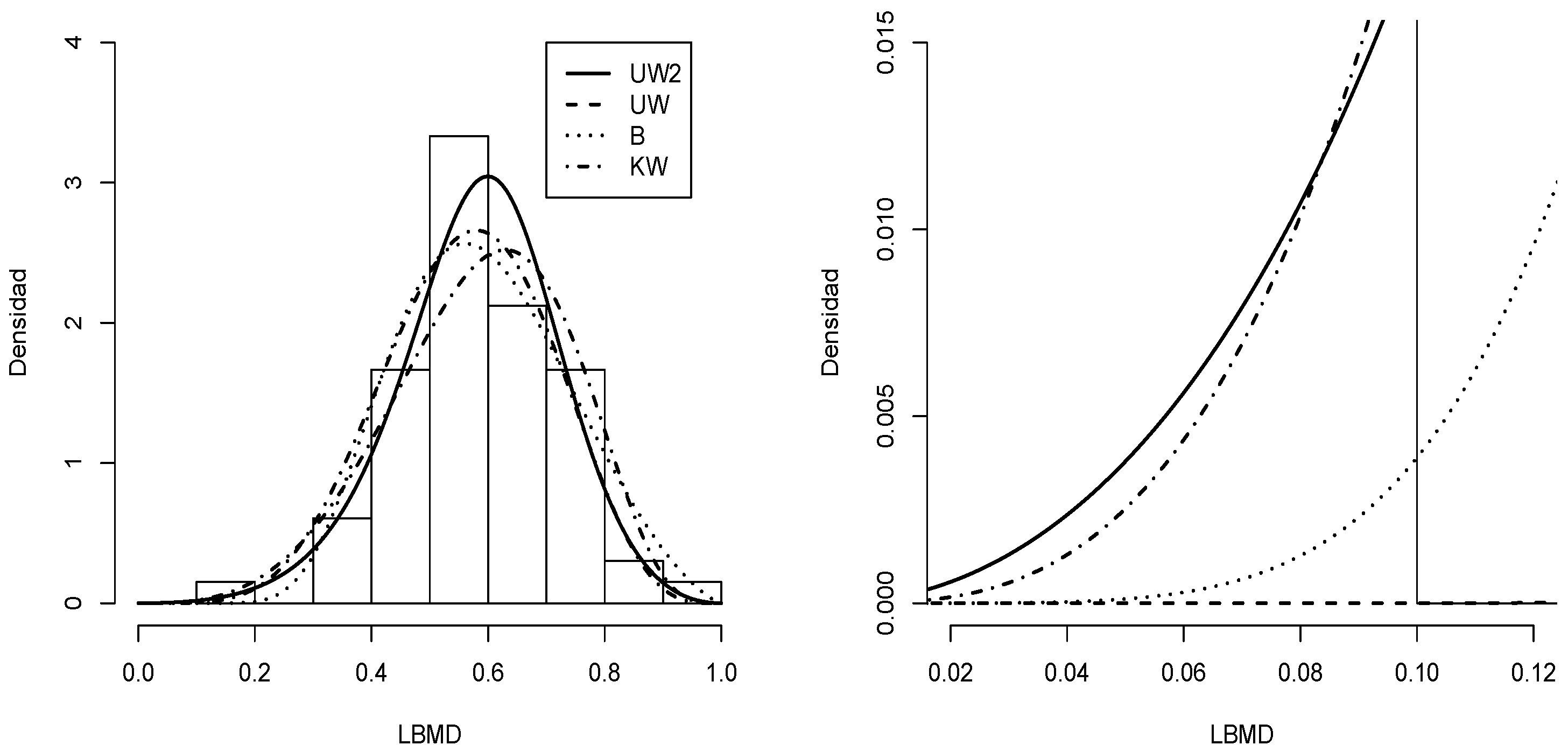
In this example, we compute the MLEs of $(\beta ,\alpha ,\theta )$ to fit the $KW$, $Beta$, $UW$, and $UW2$ models to a real data set. The data can be found in the book on Biostatistics (see [6] Daniel, Pag. 475) and correspond to a study carried out by Slemenda et al. [7], in which he investigates the effects of lateral bone mineral density (LBMD) on spinal osteoarthritis in 66 women aged 34–87 years. Some descriptive statistics are shown in Table 5. Table 6 shows the MLEs for the models: $KW$, $Beta$, $UW$, and $UW2$. Using the Akaike criterion (AIC) [8], criterion Bayesian (BIC) [9], the Kolmogorov–Smirnov (KS) test, and Chen’s approximate goodness-of-fit test [10] (W*), (A*), we see that model $UW2$ best fits the data. The advantage of the $UW2$ model is more evident for the data with more extreme observations, see Figure 10 (side right). Figure 11 and Figure 12 show that the $UW2$ distribution fits the data better than the $UW$, $Beta$, and $KW$ distributions.

Table 5. Summary statistics for ant data set of the LBMD.

n	$\overline{\mathit{w}}$	$\mathit{sd}$	${\mathit{b}}_1$	${\mathit{b}}_2$
66	0.5864	0.1339	0.04085	3.5395

Table 6. Parameters estimates for $KW$, $Beta$, $UW$, and $UW2$ distributions.

Parameter Estimates	$\mathit{KW}\left(\mathit{sd}\right)$	$\mathit{Beta}\left(\mathit{sd}\right)$	$\mathit{UW}\left(\mathit{sd}\right)$	$\mathit{UW}2\left(\mathit{sd}\right)$
$\widehat{\alpha }$	5.0241 (1.0507)	4.4717 (0.7554)	2.3068 (0.2055)	-
$\widehat{\beta }$	3.8972 (0.4386)	6.4115 (1.1016)	2.8807 (0.3867)	0.6992 (0.0513)
$\widehat{\theta }$	-	-	-	2.9370 (0.3041)
Log-likelihood	33.9586	35.5639	36.333	38.0463
AIC	−61.712	−67.1278	−68.666	−72.0926
BIC	−59.333	−62.748	−64.281	−67.713
KS Statistic	0.1212	0.1515	0.1212	0.0909
W*	0.1380	0.1029	0.08197	0.06354
A*	0.9276	0.7149	0.6091	0.4204

Figure 10. Histogram for LBMD data with Densities $UW2$ (solid line), $UW$ (dashed line), $Beta$ (dotted line), and $KW$ (dashed dotted line) (left) and tails (right).

Figure 11. QQ plots for the LBMD data set: $KW$ (a), $Beta$ (b), $UW$ (c), and $UW2$ (d).

Figure 12. Comparison of cumulative distributions for the LBMD data set for $UW2$ (blue line), $UW$ (red line), $Beta$ (green line), and $KW$ (orange line).

Observing Table 6, we see that the values of AIC and BIC are lower than those of their competitors, thus the statistic $KS$, A*, and W* indicating the best fit of the distribution $UW2$ in comparison with the distributions $KW$, $Beta$, and $UW$.

4.2. Example 2: An Application to Environment Data

In this section, we compute the MLEs of $(\alpha ,\beta ,\theta )$ to fit the $Beta$, $KW$, $UW$, and $UW2$ models to a real environment data set. The data can be found at https://dga.mop.gob.cl/servicioshidrometeorologicos/Paginas/default.aspx (1 December 2022) servicioshidrometeorologicos/Paginas/default.aspx and they correspond to the fluviometric and meteorological data recorded in monitoring stations from Arica to Tierra del Fuego. In addition, you will have access to various official statistical reports on hydrometeorological variables and water quality, obtained from our National Hydrometric Network; the analyzed data are the percentage of dissolved oxygen in a lake. Some descriptive statistics are shown in Table 7. Table 8 shows the MLEs for the models: $Beta$, $KW$, $UW$, and $UW2$. From the Akaike criteria (AIC), (BIC), we see that the $UW2$ model best fits the data. Figure 13 shows that the $UW2$ model fits the data better than $UW$, $Beta$, and $KW$ models.

Table 7. Summary statistics for environment data set of the percentage of dissolved oxygen.

n	$\overline{\mathit{w}}$	$\mathit{sd}$	${\mathit{b}}_1$	${\mathit{b}}_2$
210	0.8294	0.1283	−2.3702	11.3423

Table 8. Parameter estimates for the distributions $Beta$, $KW$, $UW$, and $UW2$.

Parameter Estimates	$\mathit{Beta}\left(\mathit{sd}\right)$	$\mathit{KW}\left(\mathit{sd}\right)$	$\mathit{UW}\left(\mathit{sd}\right)$	$\mathit{UW}2\left(\mathit{sd}\right)$
$\widehat{\alpha }$	7.3538 (0.7436)	6.9905 (0.5687)	5.4931 (0.4721)	-
$\widehat{\beta }$	1.6043 (0.1435)	1.8721 (0.0.2003)	1.1210 (0.0504)	0.1616 (0.0089)
$\widehat{\theta }$	-	-	-	2.1259 (0.1740)
AIC	−344.234	−352.005	−326.509	−394.225
BIC	−337.540	−345.311	−319.814	−387.530

Figure 13. Histogram for percent dissolved oxygen data (left) with densities of $UW2$ (solid line), $UW$ (dashed line), $Beta$ (dotted line), and $KW$ (dashed line) and tails (right).

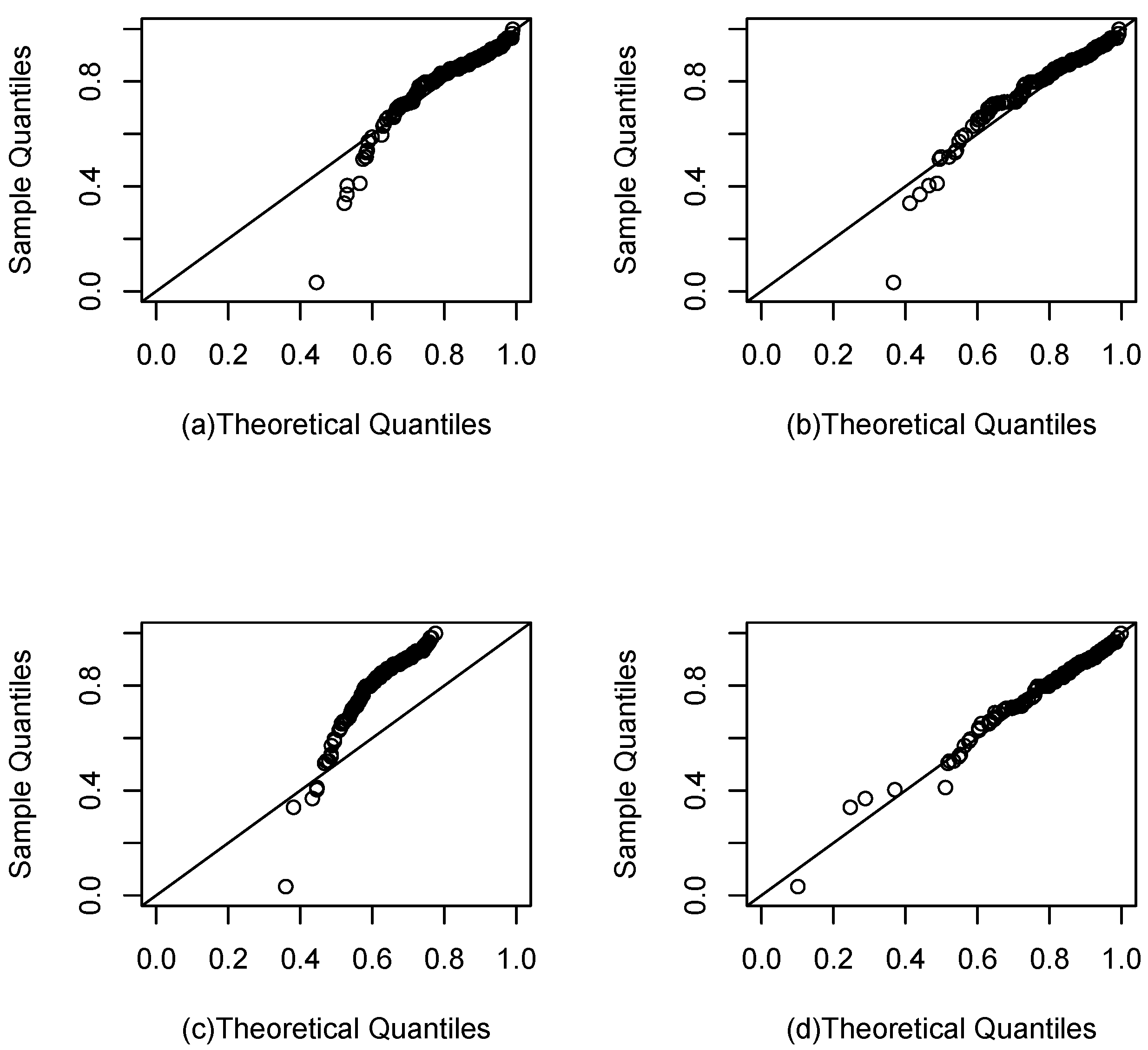
The QQ plots of the data with the $UW2$ distribution compared to the $Beta$, $KW$, and $UW2$ distributions adjusted with the maximum likelihood estimators of their parameters are shown in Figure 14.

Figure 14. QQ plots for the data set: $Beta$ (a), $KW$ (b), $UW$ (c), and $UW2$ (d).

4.3. Example 3: An Application to Quantile Regression

4.3.1. One-Dimensional Quantile Regression

Translating this concept of quantile to the regression line, we obtain the linear quantile regression (see [11]). If we assume that:

$$\begin{array}{ccc}\hfill Y_i& =& {\alpha }_{0,\tau }+{\alpha }_{1,\tau }{X}_i+{ϵ}_{i,\tau },\forall iϵ(1,...,n),\hfill \end{array}$$

(50)

with $\tau ϵ(0,1)$ and that the conditional expected value is not necessarily zero, but the $\tau$-th quantile of the error with respect to the return variable is zero $(Q_{\tau }\left({ϵ}_{i,\tau }\right|X)=0)$, so the $\tau$-th quantile of $Y_i$ with respect to X can be written as:

$$\begin{array}{ccc}\hfill Q_{\tau }\left(Y_i\right|X)& =& {\alpha }_{0,\tau }+{\alpha }_{1,\tau }{X}_i.\hfill \end{array}$$

(51)

The estimators of ${\alpha }_{0,\tau }$ and ${\alpha }_{1,\tau }$ are obtained by:

$${\widehat{\alpha }}_{\tau }=arg\underset{{\alpha }_{\tau }ϵ{\Re }^2}{min}\left(\sum _{Y_i\ge A}\tau |Y_i-{\alpha }_{0,\tau }-{\alpha }_{1,\tau }{X}_i|+\sum _{Y_i<A}(1-\tau )|Y_i-{\alpha }_{0,\tau }-{\alpha }_{1,\tau }{X}_i|\right),$$

(52)

being ${\alpha }_{\tau }=({\alpha }_{0,\tau },{\alpha }_{1,\tau })$ and $A={\alpha }_{0,\tau }+{\alpha }_{1,\tau }{X}_i$. To estimate the parameters, the function described in the formula must be minimized.

4.3.2. Quantile Regression Unitary Weibull Type 2

In this case, in the regression equation:

$$\begin{array}{ccc}\hfill Y_i& =& {\alpha }_{0,\tau }+{\alpha }_{1,\tau }{X}_i+{ϵ}_{i,\tau },\forall iϵ(1,...,n),\hfill \end{array}$$

(53)

where the response variable $Y\sim UW2(\theta ,\beta )$, it is possible to reparameterize it in the distribution. So, one way to obtain the quantile of the function of Y is the following:

Let ${\mu }_{\tau }={\left[1+\beta {\left(\frac{1}{\tau }-1\right)}^{\frac{1}{\theta }}\right]}^{-1}$, then $\beta =\left({\displaystyle \frac{1-{\mu }_{\tau }}{{\mu }_{\tau }}}\right){\left({\displaystyle \frac{\tau }{1-\tau }}\right)}^{1/\theta }$ and substituting into the density function of Y, we obtain:

$$\begin{array}{c}\hfill f_Y\left(y\right)=\frac{\theta {\left({\displaystyle \frac{1-{\mu }_{\tau }}{{\mu }_{\tau }}}\right)}^{\theta }\left({\displaystyle \frac{\tau }{1-\tau }}\right)y^{\theta -1}{(1-y)}^{\theta -1}}{{\left[{\left({\displaystyle \frac{1-{\mu }_{\tau }}{{\mu }_{\tau }}}\right)}^{\theta }\left({\displaystyle \frac{\tau }{1-\tau }}\right)y^{\theta }+{(1-y)}^{\theta }\right]}^2},0<y<1,\end{array}$$

(54)

then the cdf of Y is:

$$\begin{array}{c}\hfill F_Y\left(y\right)={\left[1+\frac{{\left(\frac{1-\tau }{\tau }\right)}^{\theta +1}}{\frac{1-{\mu }_{\tau }}{{\mu }_{\tau }}}\right]}^{-1}.\end{array}$$

(55)

then $Y\sim UW2({\mu }_{\tau },\theta )$, where $0<{\mu }_{\tau }<1$ is the quantile parameter. Considering $\tau$ known, ${\mu }_{\tau }$ and $\theta$ are estimated by the maximum likelihood.

4.3.3. An Application of Quantile Regression to Praters Gas Mileage Data

To illustrate this, we consider Simas et al. [12] investigating Praters gas mileage data based on the same mean equation as above, but now with temperature. Table 9 shows the statistics of these data. Table 10 shows the maximum likelihood estimators as predictor variables of $({\alpha }_0,{\alpha }_1)$ and their standard errors for the $UW2$, $UW$, and $Beta$ distributions.

Table 9. Summary statistics for data set of the temperature and yield.

$\mathit{Data}$	n	$\overline{\mathit{w}}$	$\mathit{sd}$	${\mathit{b}}_1$	${\mathit{b}}_2$
Yield	52	332.0938	69.7559	−0.2657	1.3058
Temp	52	0.1965	0.1070	0.3687	2.1997

Table 10. Parameters estimates and standard error for the quantile regression coefficients $UW2$, $UW$, and $Beta$ models for the dataset and the quantile of 0.5.

			$\mathit{UW}2$				$\mathit{UW}$				$\mathit{Beta}$
$\mathit{Coef}.$	$\mathit{Est}.$	$\mathit{sd}$	t-Value	p-Value	$\mathit{Est}.$	$\mathit{sd}$	t-Value	p-Value	$\mathit{Est}.$	$\mathit{sd}$	t-Value	p-Value
${\alpha }_0$	−0.1702	0.0800	−2.1256	0.0418	−0.1733	0.0963	−1.7992	0.0820	−0.1339	0.0528	−2.5333	0.0167
${\alpha }_1$	0.0011	0.0002	4.1976	0.0002	0.0012	0.0003	3.6745	0.0009	0.0009	0.0001	5.1823	0.0000

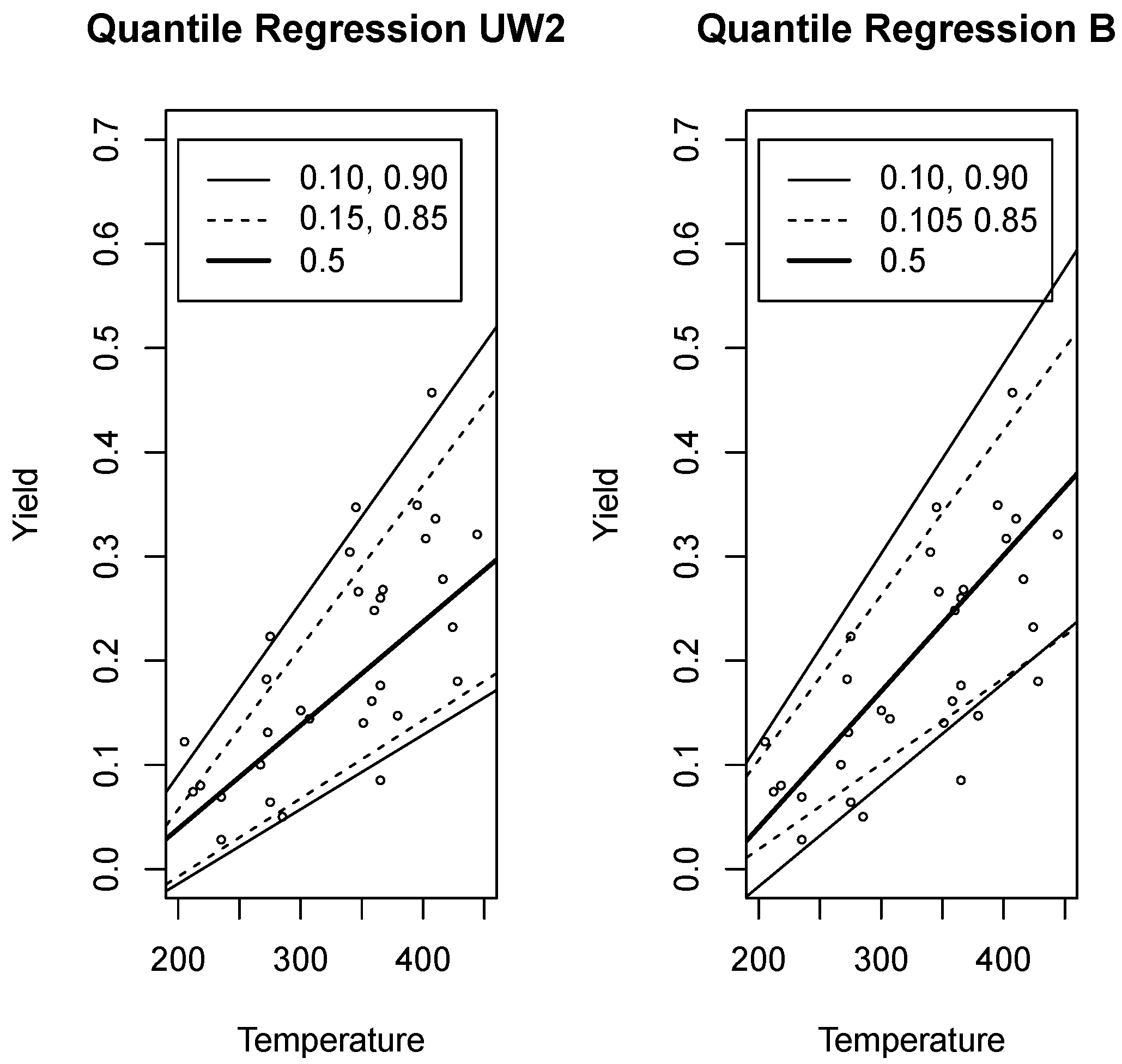
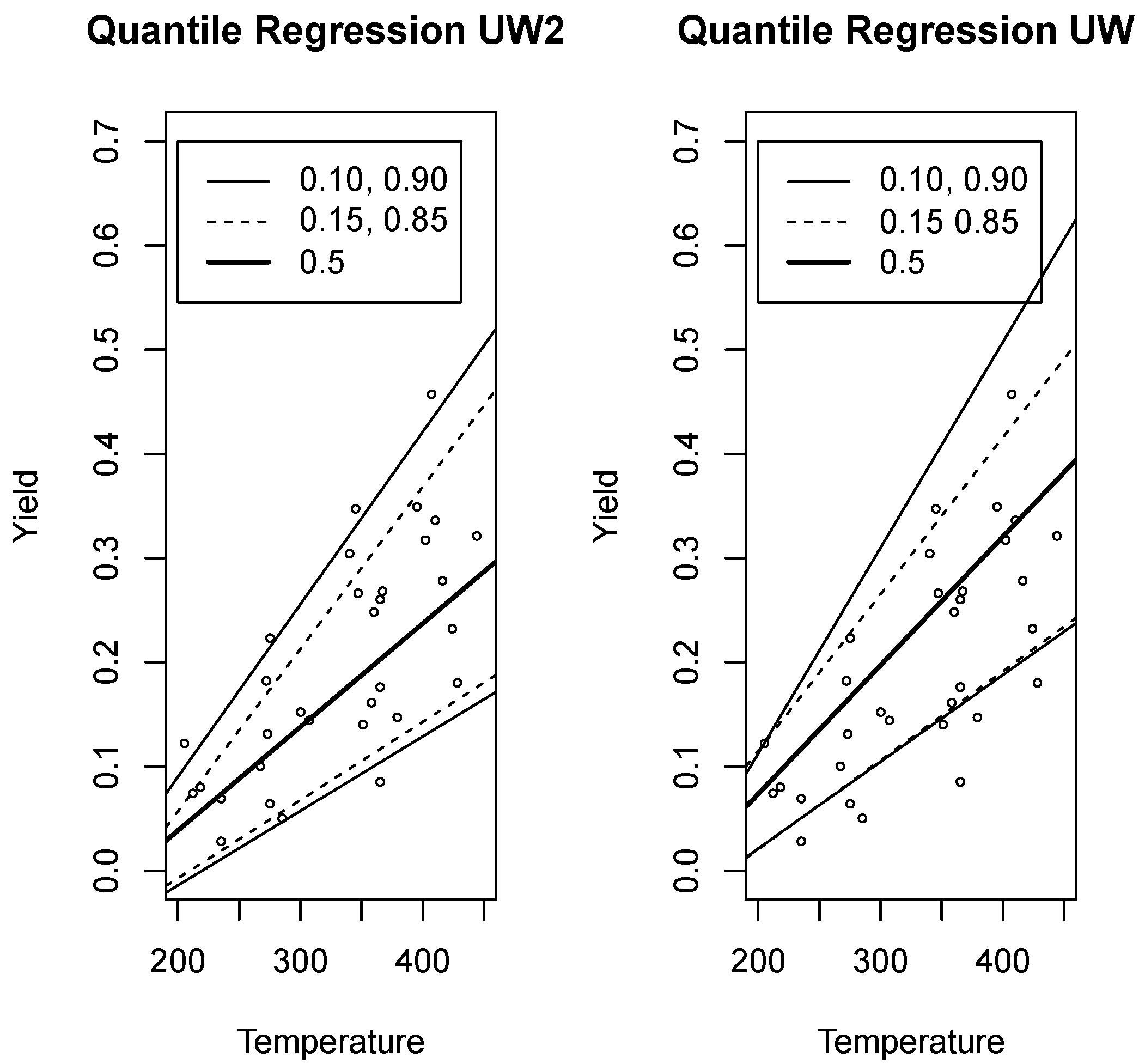
Looking at Table 11 and Figure 15 and Figure 16, we see that the $UW2$ distribution compared to the $Beta$ and $UW$ distributions fits better using quantile regression when the variable response has high kurtosis.

Table 11. AIC and BIC values for the models $UW2$, $UW$, and $Beta$ of the Temperature and Yield.

Model	AIC	BIC
$UW2$	−58.07373	−53.67652
$UW$	−53.75805	−49.36084
$Beta$	−43.69310	−39.29589

Figure 15. Quantile regression for Yield and Temperature data with $UW2$ density (left) and $Beta$ density (right).

Figure 16. Quantile regression for Yield and Temperature data with $UW2$ density (left) and $UW$ density (right).

5. Discussion

In this work, we have introduced a new family of distributions with a domain in the interval (0,1) and with heavier tails than some similar distributions seen in the literature. The new family is based on a transformation of two independent random variables with a two-parameter Weibull distribution. We define the new family by its stochastic representation. We provide its density function and reliability function and also provide some statistical properties of interest. In the inferential part, we estimate the parameters of the new model using the maximum likelihood method and the information criteria are used to select the best model and evaluate the goodness of fit of the new distribution compared to other similar distributions. A Monte Carlo simulation study was carried out to empirically evaluate the statistical performance of the estimators, using the maximum likelihood method for the parameters of the new model. In addition, we show the coverage probabilities and the mean length of the confidence intervals obtained for the corresponding parameters using the asymptotic normality of these estimators. The simulation study reported consistent performance of these estimators. Finally, three illustrations with real data were created, with two related to medical information and the environment. A third application was related to quantile regression. These analyses provided sufficient information to conclude that the proposed model presents better behavior when compared to others from the competition.

References

- Kumaraswamy, P. A generalized probability density function for double-bounded random processes. J. Hydrol. 1980, 46, 79–88. [Google Scholar] [CrossRef]
- Mazucheli, J.; Menezes, A.F.B.; Ghitany, M.E. The unit-Weibull distribution and associated inference. J. Appl. Probability Stat. 2018, 13, 1–22. [Google Scholar]
- Mazucheli, J.; Menezes, A.F.B.; Fernandes, L.B.; de Oliveira, R.P.; Ghitany, M.E. The unit-Weibull distribution as an alternative to the Kumaraswamy distribution for the modeling of quantiles conditional on covariates. J. Appl. Stat. 2019, 47, 954–974. [Google Scholar] [CrossRef]
- Butler, R.J.; McDonald, J.B. Using incomplete moments to measure inequality. J. Econom. 1989, 42, 109–119. [Google Scholar] [CrossRef]
- Gastwirth, J.L. The Estimation of the Lorenz Curve and Gini Index. Econ. Stat. 1972, 54, 306–316. [Google Scholar] [CrossRef]
- Daniel, W.W. Biostatistics: A Foundation for Analysis in the Health Sciences, 9th ed.; John Wiley and Sons, Inc.: Hoboken, NJ, USA, 2005. [Google Scholar]
- Slemenda, C.W.; Turner, C.H.; Peacock, M.; Christian, J.C.; Sorbel, J.; Hui, S.L.; Johnston, C.C. The genetics of proximal femur geometry, distribution of bone mass and bone mineral density. Osteoporos. Int. 1996, 6, 178–182. [Google Scholar] [CrossRef]
- Akaike, H. A new look at the statistical model identification. IEEE Trans. Autom. Control 1974, 19, 716–723. [Google Scholar] [CrossRef]
- Schwarz, G. Estimating the dimension of a model. Ann. Stat. 1978, 6, 461–464. [Google Scholar] [CrossRef]
- Chen, G.; Balakrishnan, N. A general Purpose Aproximate Goodness-of-Fit Test. J. Qual. Technol. 1995, 27, 154–161. [Google Scholar] [CrossRef]
- Buchinsky, M. Quantile regression, Box-Cox transformation model, and the U.S. wage structure. J. Econom. 1995, 65, 109–154. [Google Scholar] [CrossRef]
- Simas, A.B.; Barreto-Souza, W.; Rocha, A.V. Improved Estimators for a General Class of Beta Regression Models. Comput. Stat. Data Anal. 2010, 54, 348–366. [Google Scholar] [CrossRef]
Disclaimer/Publisher’s Note: The statements, opinions and data contained in all publications are solely those of the individual author(s) and contributor(s) and not of MDPI and/or the editor(s). MDPI and/or the editor(s) disclaim responsibility for any injury to people or property resulting from any ideas, methods, instructions or products referred to in the content. |
© 2023 by the authors. Licensee MDPI, Basel, Switzerland. This article is an open access article distributed under the terms and conditions of the Creative Commons Attribution (CC BY) license (https://creativecommons.org/licenses/by/4.0/).