Abstract
The primary objective of this article was to introduce a new probabilistic model for the discussion and analysis of random covariates. The introduced model was derived based on the Marshall–Olkin shock model. After proposing the mathematical form of the new bivariate model, some of its distributional properties, including joint probability distribution, joint reliability distribution, joint reversed (hazard) rate distribution, marginal probability density function, conditional probability density function, moments, and distributions for both and , were investigated. This novel model can be applied to discuss and evaluate symmetric and asymmetric data under various kinds of dispersion. Moreover, it can be used as a probability approach to analyze different shapes of hazard rates. The maximum likelihood approach was utilized for estimating the parameters of the bivariate model. A simulation study was carried out to assess the performance of the parameters, and it was noted that the maximum likelihood technique can be used to generate consistent estimators. Finally, two real datasets were analyzed to illustrate the notability of the novel bivariate distribution, and it was found that the suggested distribution provided a better fit than the competitive bivariate models.
Keywords:
statistical model; Marshall–Olkin shock model; marginal distributions; simulation; comparative study; statistics and numerical data MSC:
60E05; 62H12; 62P99
1. Introduction
In the field of statistics, data are classified according to the number of variables in a given study. Depending on how many variables are being considered, the data may be univariate, “single variable/factor”, or it may be bivariate, “double variables/factors”. Bivariate data can also be two sets of items that are dependent on each other. These data are one of the simplest forms of statistical analysis and are used to see if there is a relationship between two sets of values and . Furthermore, the bivariate data could be temperatures in two different regions, droughts in two different regions, grades for two different educational courses, two teams’ results per year, etc. Because of these situations, many statisticians aim to create flexible bivariate/joint probability models for discussing and analyzing such data.
To generate a bivariate model, there are different methods that can be used. One of these techniques is called the shock model (see Marshall and Olkin “MO”, [1]). For a discussion of the MO technique, suppose we have three independent sources of shocks, and that these shocks affect a two-component system. The shock from source number one is supposed to reach the system and destroy the first component instantly, and the shock from the second source reaches the system and destroys the second component instantly, but if the shock from the third source hits the system, it instantly destroys both components. Given the importance of this approach, many statisticians have applied it to construct a bivariate probability structure. For instance, Domma [2] presented a bivariate MO Burr type III distribution, Sarhan et al. [3] derived a bivariate MO-generalized linear failure rate model, Barreto-Souza and Lemonte [4] introduced a bivariate MO Kumaraswamy family/class of distributions, Kundu and Gupta [5] discussed a bivariate MO Weibull geometric model, Shahen et al. [6] proposed a bivariate MO exponentiated modified Weibull distribution, Eliwa and El-Morshedy [7,8] derived and studied two bivariate MO generators based on Gumbel-G and odd Weibull-G families, Franco et al. [9] introduced a bivariate MO generator based on Burr type X and inverted Kumaraswamy classes, Tahir et al. [10] discussed a bivariate MO for a new Kumaraswamy generalized family, El-Morshedy et al. [11] discussed a bivariate MO generator for a unit interval of , Kundu [12] proposed a semi-parametric singular class based on MO approach, etc.
Although there are many bivariate MO models mentioned in the statistical literature, there is room for creating bivariate models that are more appropriate to discuss the complex data that are generated day in and day out. From this point of view, the authors planned to derive a flexible bivariate model that could be used as a utility for statisticians interested in discussing bivariate data under different formats. To achieve this goal, the exponentiated inverse flexible Weibull extension (for short, EIFWE) model (El-Morshedy et al., [13]) was used as a baseline model of the MO technique, and consequently, the generated model is called a bivariate EIFWE (for short, BEIFWE). The cumulative distribution function (CDF) and its corresponding probability density function (PDF) of the EIFWE model can be determined, respectively, as follows:
and
The method proposed in this paper can be applied for the following reasons: Joint PDF and joint CDF can be expressed in closed forms, which makes the application more convenient in practice; the joint PDF and joint hazard rate functions (HRFs) can take different forms depending on the values of their parameters; margin can be used to analyze different forms of failure rates; the model can be applied quite easily if there are links/ties in the data; and the model can be utilized to discuss symmetric and asymmetric datasets under different forms of scattering.
The article unfolds as follows: In Section 2, the mathematical structure of the BEIFWE model is derived. Some statistical properties of the BEIFWE distribution are discussed in Section 3. In Section 4, the parameters of the BEIFWE model are estimated by utilizing the maximum likelihood method. A simulation study is performed in Section 5. The usefulness of the BEIFWE distribution and its testing across two real datasets is illustrated in Section 6. Finally, some concluding remarks and future work are listed in Section 7.
2. Structure of the BEIFWE Model
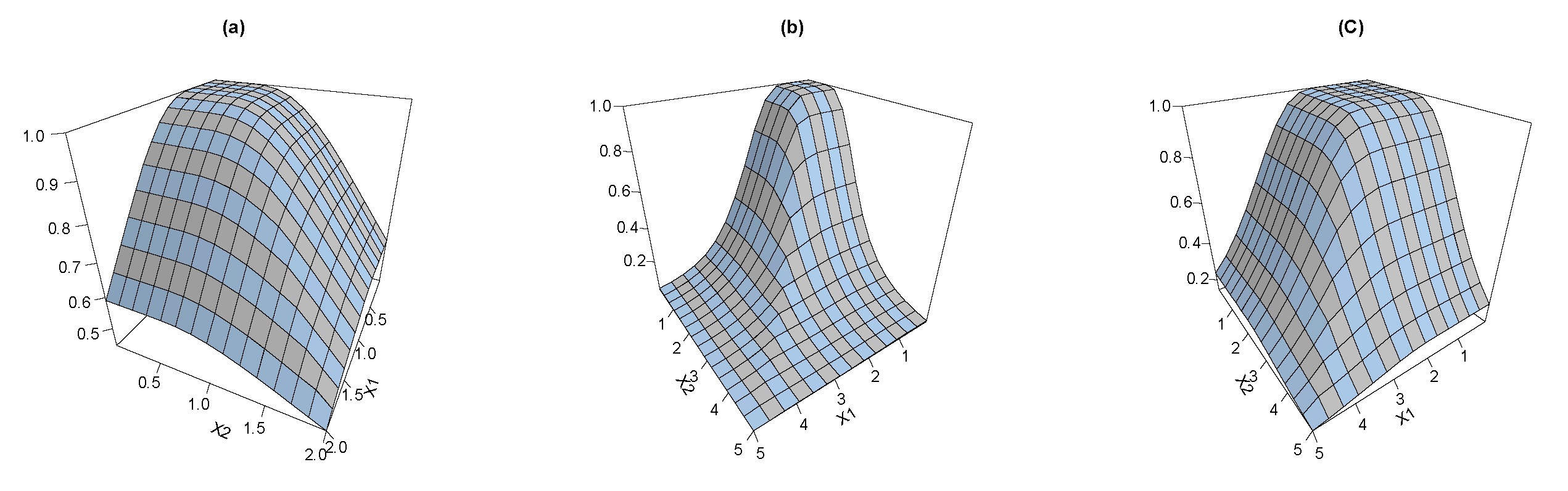
Suppose are three independent random variables (RVs) such that EIFWE (). Define and . Then, the bivariate vector “BVr” has a BEIFWE distribution with parameters , e.g., BEIFWE .The joint CDF of the BVr is given as
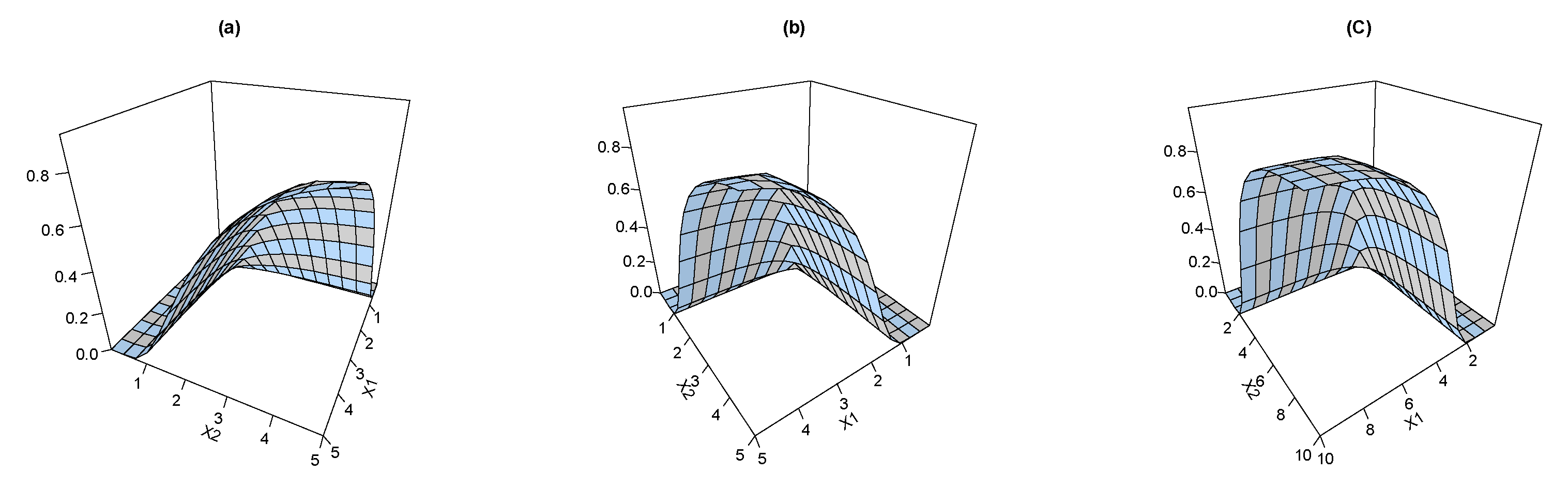
where Figure 1 shows the joint CDF plots for the BEIFWE model based on various values of the BEIFWE parameters “a: ”; “b: ”; and “c: ”.
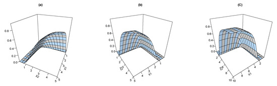
Figure 1.
The joint CDF of the BEIFWE distribution.
The joint PDF corresponding to Equation (3) can be listed as
where
and
To derive Equation (4), assume that ; then, the expression for can be obtained by differentiating the joint CDF given in Equation (3) with respect to and Similarly, for . However, cannot be derived in a similar approach. For this reason, when the following formula can be applied to derive
where
and
then
Thus,
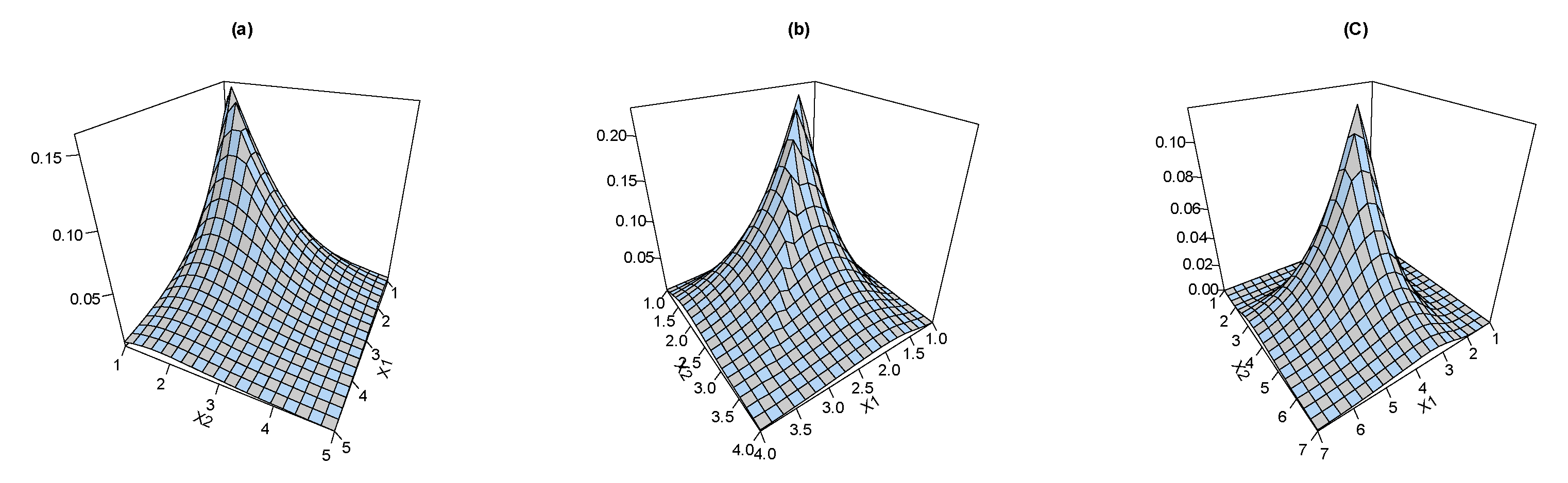
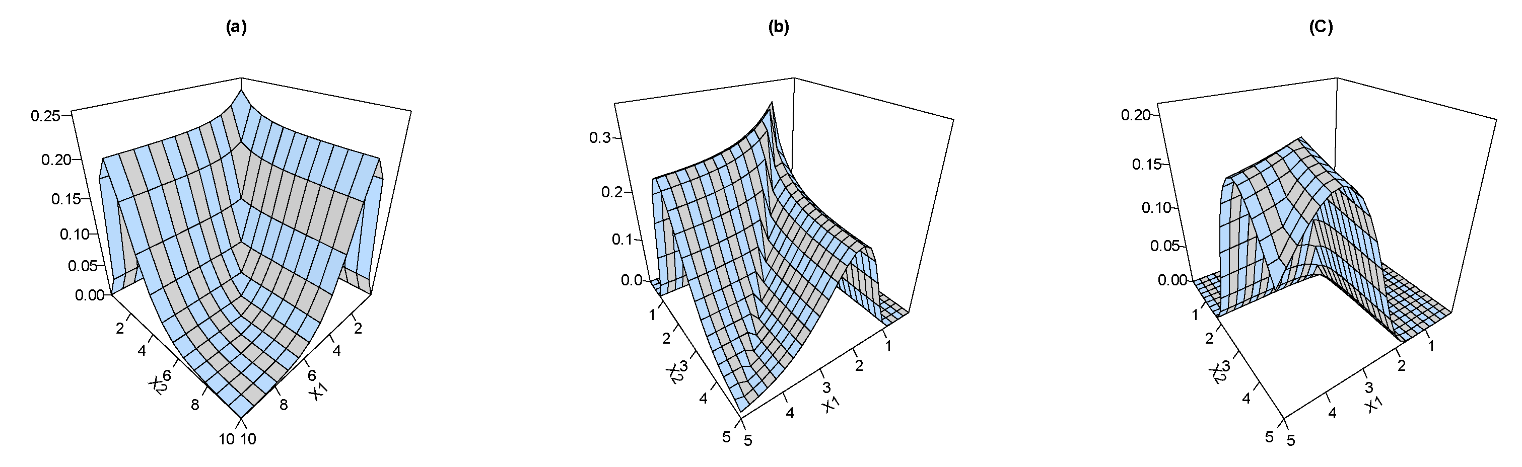
Figure 2 shows the joint PDF plots for the BEIFWE model based on various schemas “a: ”; “b: ”; and “c: ”.
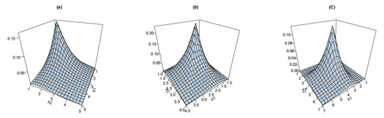
Figure 2.
The joint PDF of the BEIFWE distribution.
The joint PDF of the BEIFWE model can take different forms depending on the values of its parameters. Thus, the proposed probability tool can be applied to analyze various types of datasets in different fields including symmetric and asymmetric observations.
3. Distributional Properties
3.1. Joint Reliability and Joint (Reversed) Hazard Rate Functions
Assume the random vector (RmVr) has the BEIFWE distribution; then, the joint RF can be expressed as
where
and
Equation (7) can be derived utilizing the following relation:
Figure 3 shows the joint RF plots for the BEIFWE according to different schemas “a: ”; “b: ”; and “c: ”.
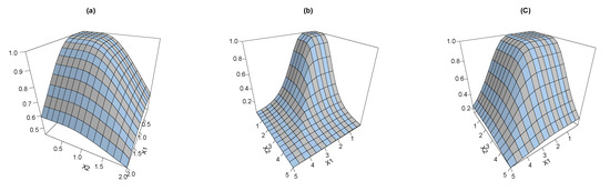
Figure 3.
The joint RF of the BEIFWE distribution.
The joint HRF corresponding to Equation (7) can be expressed as
where
and
Equation (9) can be derived using ; more details on the joint HRF are provided in a study by Basu, [14]). Figure 4 shows the joint HRF plots for the BEIFWE based on various schemes “a: ”, “b: ” and “c: ”.

Figure 4.
The joint HRF of the BEIFWE distribution.
As we can see, the joint HRF of the BEIFWE model can take various shapes depending on the values of its parameters. Thus, the presented distribution can be utilized to discuss different kinds of datasets in several fields. The corresponding joint reversed HRF “RHRF” to Equation (7) can be formulated as
where
and
Equation (10) can be derived using ; for more detail on the RHRF, readers can refer to Bismi, [15].
3.2. Marginal Probability Density Functions
Lemma 1.
If the RmVr have a BEIFWE , then the marginal PDFs of can be proposed as
where and
Proof.
Since the marginal CDFs for can be defined by
and the RVs are mutually independent, we directly obtain
Then, it is easy to obtain the marginal PDFs where . □
3.3. The Distribution of and
Consider that the RmVr has the BEIFWE distribution; then, the CDF for the RV Y and W can be expressed as
and
The distributions of the RVs Y and W can be used in reliability theory, especially in manufacturing and maintenance. Another application of the RVs Y and is that they can be applied to read and evaluate signals received from space via satellites.
3.4. Conditional Probability Density Functions
Lemma 2.
Assume the RVr has the BEIFWE ; then, the conditional PDF of given ,
can be expressed as
where
and
Proof.
It is easy to prove this lemma by using the following relation:
□
3.5. Marginal Expectation
Lemma 3.
Consider that the RVr has a BEIFWE distribution; then, the moment of can be formulated as
4. Maximum Likelihood Estimation (MLE)
In this segment, the technique of maximum likelihood is applied to estimate the unknown parameters of the BEIFWE distribution. Suppose we have a sample of size n in the form , ,..., from the BEIFWE distribution. We utilize the following notations: , , , ,, , and Based on the observations, the likelihood function is given as
The log-likelihood function can be written as
Using Equation (18) to obtain the first partial derivatives with respect to , and and setting the results equal zeros, we obtain the likelihood equations in the following form:
and
To determine the MLEs of the parameters , and , we have to solve the above system of five non-linear equations. A numerical technique should be used to solve these equations.
5. MLE Performance: A Simulation Study
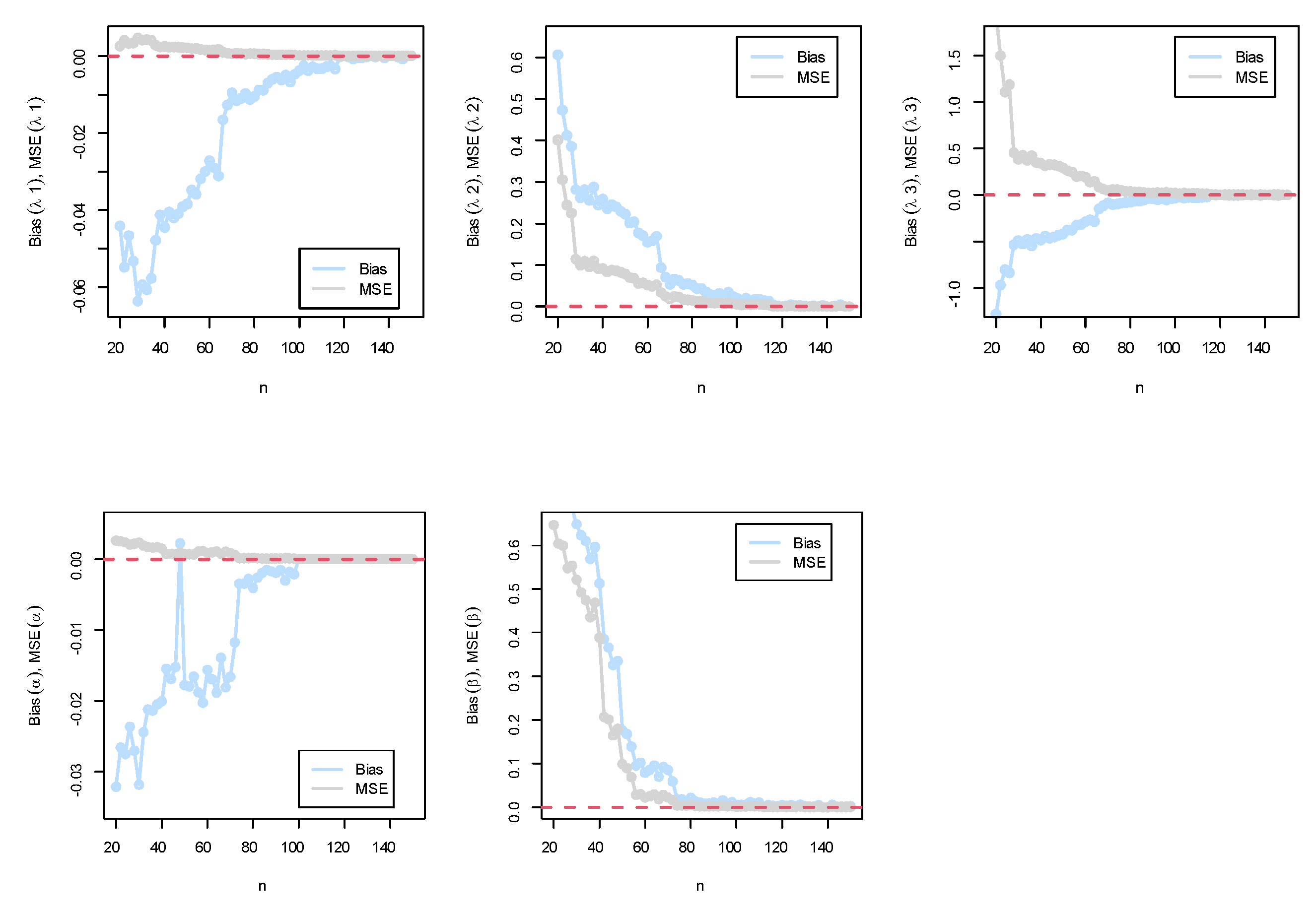
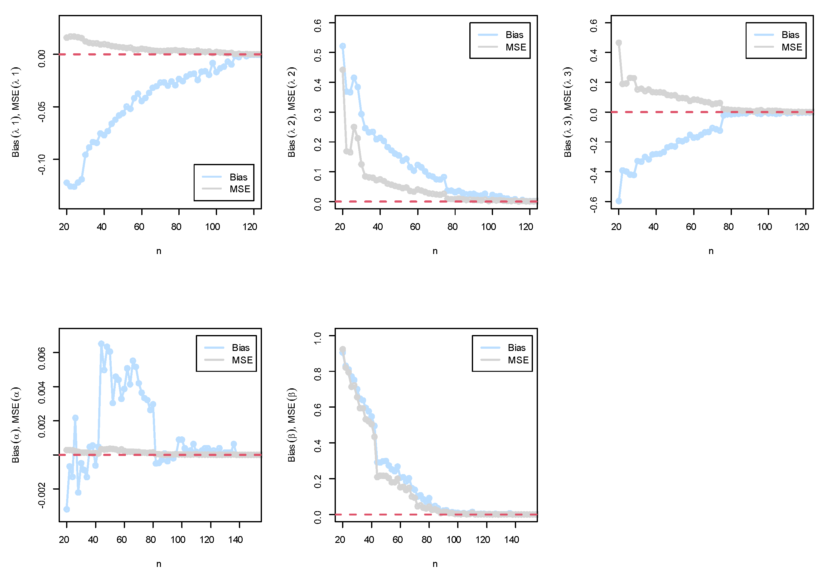
In this segment, the MLE approach was used to estimate the parameters , and of the BEIFWE distribution under different sample sizes from N = 10,000 replications. The generated samples were based on the quantile function of the marginal distributions of the BEIFWE model. The population parameters were generated utilizing the R software package. The primary aim of this section is to introduce an assessment of the properties of the MLE in terms of bias and mean-squared error (MSE) for the parameters. To test the performance of the MLE technique, two schemes are considered and discussed under different sample sizes. The experimental schemas can be formulated as follows:
- Schema I: BEIFWE();
- Schema II: BEIFWE().
The empirical results can be displayed in Figure 5.
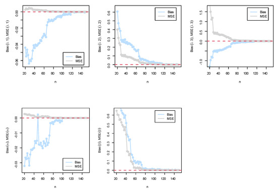
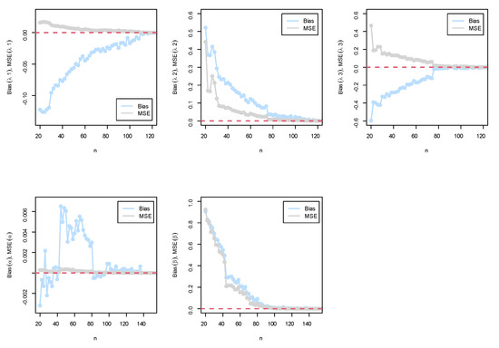
Figure 5.
(Top) simulation results of the BEIFWE (0.5,0.7,0.9,0.2,0.5) model; (bottom) simulation results of the BEIFWE (0.2,0.4,0.6,0.8,1.1) model.
The following observations can be noted: The MSEs for the MLE always decreased to zero when n grew, and the magnitude of bias, in general, was always close to zero when n grew. Based on the MSE, the performance of the MLE approach was good, and the confidence in the results increased as the sample size increased.
6. Comparative Study: Statistics and Real Data Analysis
In this section, we illustrate the importance of the BEIFWE distribution using two applications of real data. The fitted distributions were compared with several famous bivariate models to explicate that the BEIFWE distribution can be a good lifetime model, comparing with bivariate Gompertz (BGz) (Al-Khedhairi and El-Gohary, [16]), bivariate Burr X bivariate Gompertz (BBUXGz) (El-Morshedy et al., [17]), bivariate generalized exponential (BGE) (Kundu and Gupta, [18]), Marshall–Olkin bivariate exponential (MOBE) (Marshall and Olkin, [1] and Jose, [19]), bivariate exponentiated Weibull (BEW), bivariate Gumbel exponential (BGuE) (Eliwa and El-Morshedy, [7]), bivariate generalized linear failure rate (BGLFR) (Sarhan et al., [3]), bivariate generalized Gompertz (BGGz) (Al-Khedhairi and El-Gohary, [16]), bivariate Burr X bivariate exponential (BBUXE) (El-Morshedy et al., [17]), bivariate exponentiated Weibull–Gompertz (BEWGz) (El-Bassiouny et al. [20]), bivariate Gumbel Gompertz (BGuGz) (Eliwa and El-Morshedy, [7]), bivariate exponentiated modified Weibull extension (BEMWEx) (El-Gohary et al., [21]), and bivariate Weibull exponential (BWE) (Hanagal, [22]) distributions. The fitted models were compared utilizing some criteria, namely the negative maximized log-likelihood (), Akaike information criterion (AIC), corrected AIC (CAIC), Bayesian IC (BIC), and Hannan–Quinn IC (HQIC), in addition to the Kolmogorov–Smirnov (KS) statistic and its p-value for the marginals.
6.1. Dataset I: Football Data
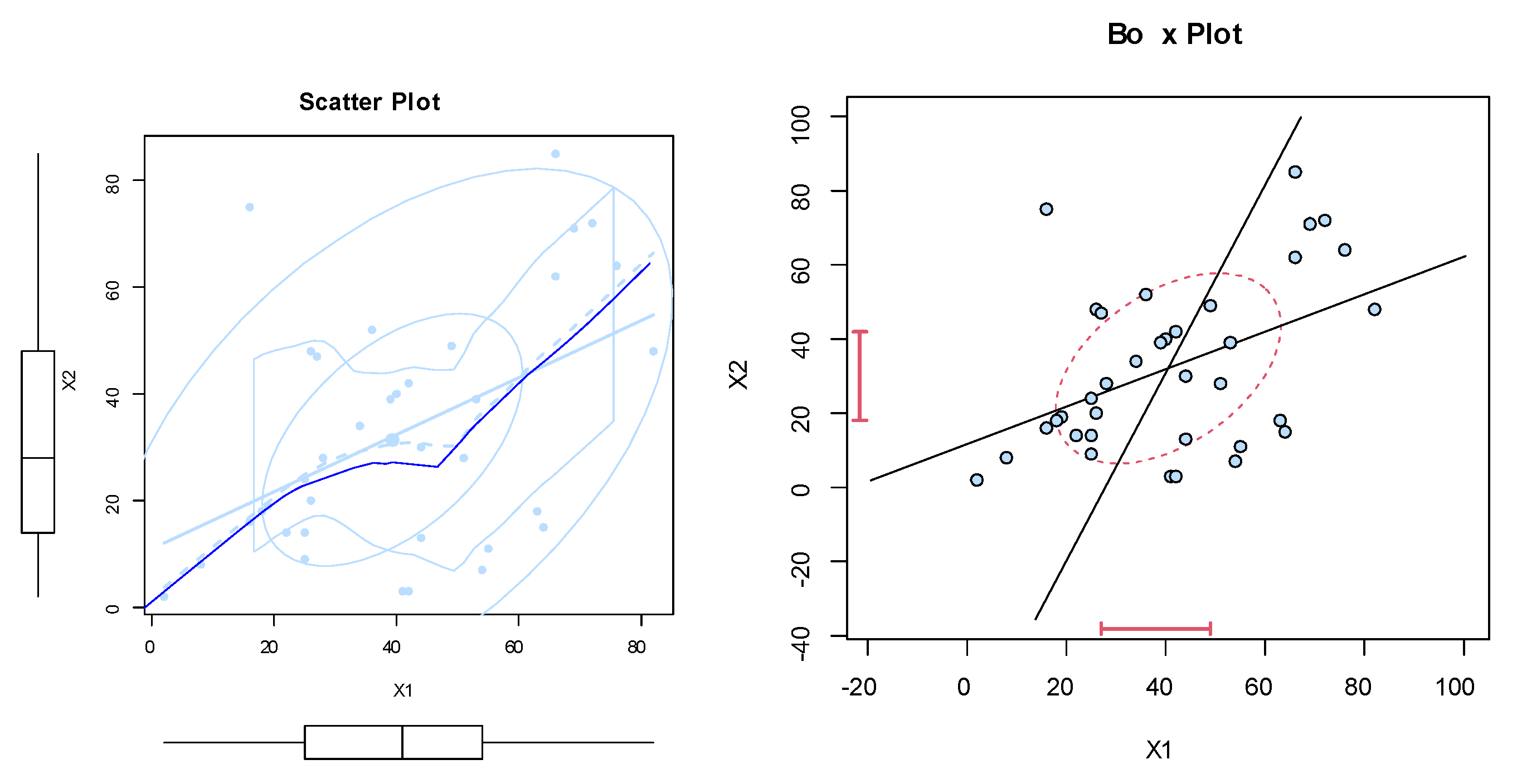
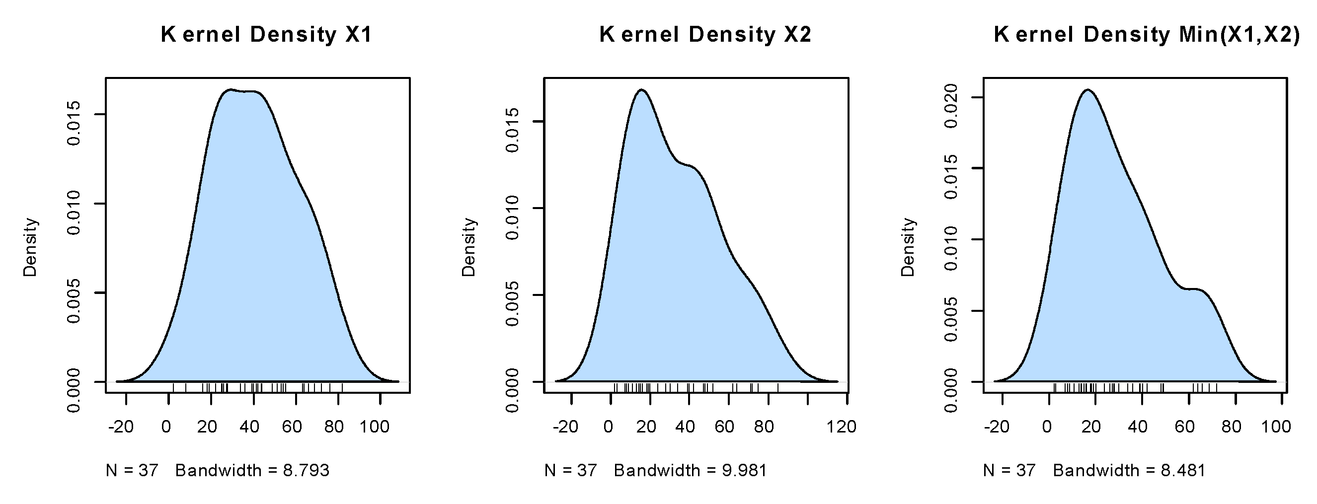
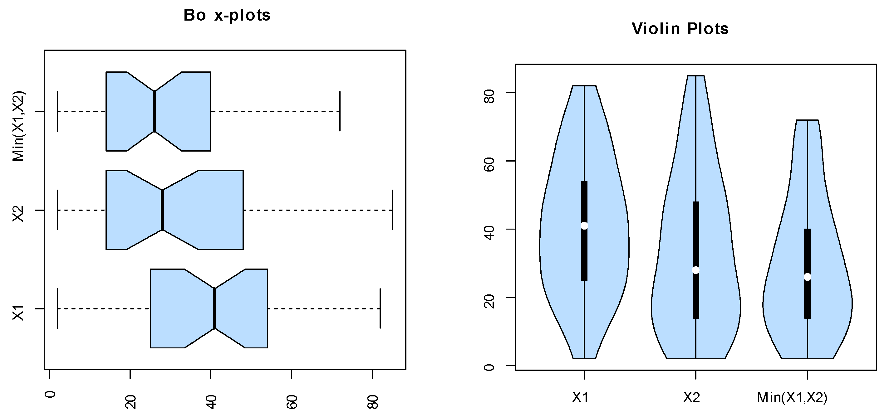
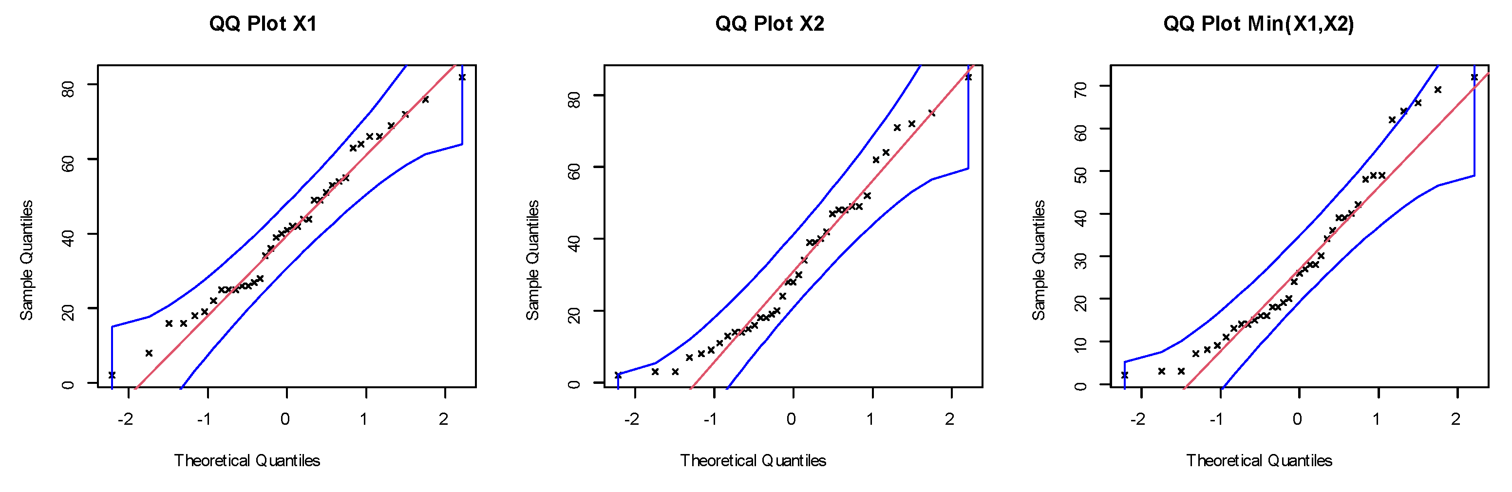
The dataset was obtained from Meintanis [23]. These data represent football (soccer) data from the UEFA Champions League. They represent soccer data for when at least one goal is scored by a kick goal (such as a penalty kick, foul kick, or any other direct kick) by any team, and one goal is scored by the home team. Here, represents the bivariate data, where represents the time in minutes of the first kick goal scored by any team, and represents the first goal scored by the home team. Note that all possibilities are there, namely (i) , (ii) , and (iii) . Nonparametric plots are listed in Figure 6, Figure 7, Figure 8 and Figure 9 to discuss the behavior of data. Figure 6 shows the scatter and box plots for the bivariate data, whereas the kernel densities, violin, box, and quantile–quantile (QQ) plots for the marginals are displayed in Figure 7, Figure 8 and Figure 9.
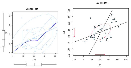
Figure 6.
The scatter and box plots of dataset I.
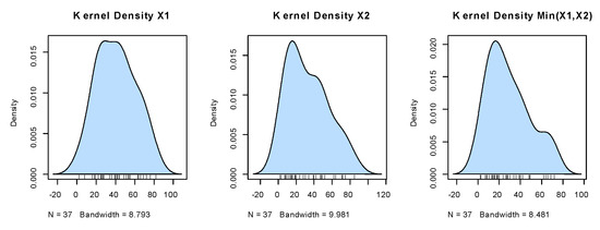
Figure 7.
The kernel densities for the marginals of dataset I.

Figure 8.
The box and violin plots for the marginals of dataset I.
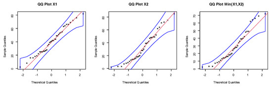
Figure 9.
The QQ plots for the marginals of dataset I.
Before trying to analyze the data using the BEIFWE model, first, we fit the marginals , , and min() separately on the UEFA Champions League data. The MLEs of the parameters for , , and min() are (0.3300, 0.05432, 5.3005), (1.3062, 0.0479, 2.5079), and (2.7244, 1.1797, 0.0569), respectively. The , K-S, and its p-value for the marginals , , and min() can be listed as (163.4554, 0.09218, 0.9116), (162.7615, 0.1026, 0.8308), and (157.6972, 0.0636, 0.9983), respectively. Based on p-values, it is clear that the BEIFWE model fits the data for the marginals. Figure 10, Figure 11 and Figure 12 show the fitted PDFs, the estimated CDF, and probability–probability (PP) plots for the marginals , , and min(), which prove our results.
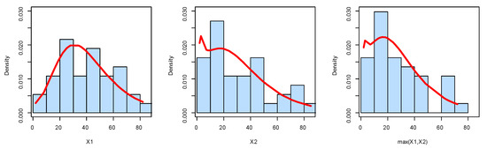
Figure 10.
The fitted PDF plots for the marginals of dataset I.
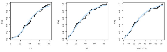
Figure 11.
The estimated CDF plots for the marginals of dataset I.
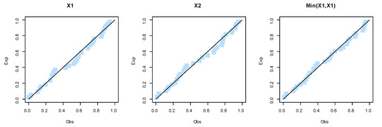
Figure 12.
The fitted PP plots for the marginals of dataset I.
Now, we fit the BEIFWE model on these data. In the enclosed Table 1 and Table 2, we provide the MLEs, , AIC, CAIC, BIC, and HQIC values for the competitive distributions.

Table 1.
The MLEs for the competitive distributions’ parameters.
Table 2.
The goodness-of-fit results for the competitive distributions.
As we can see, the BEIFWE distribution fits the data better than the other tested models, because it has the smallest value among , AIC, CAIC, BIC, and HQIC.
6.2. Dataset II: Motor Data
These data are reported in Relia [24], and they represent the failure times of a parallel system constituted by two identical motors in days. Nonparametric plots are reported in Figure 13, Figure 14, Figure 15 and Figure 16 to discuss the shape of data. Figure 13 shows the scatter and box plots for data, whereas the kernel densities, violin, box, and QQ plots for the marginals are listed in Figure 14, Figure 15 and Figure 16.
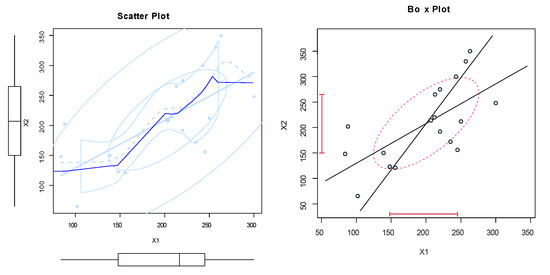
Figure 13.
The scatter and box plots of dataset II.
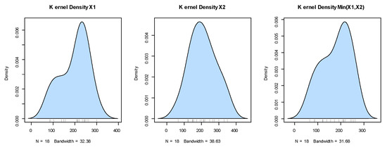
Figure 14.
The kernel densities for the marginals of dataset II.
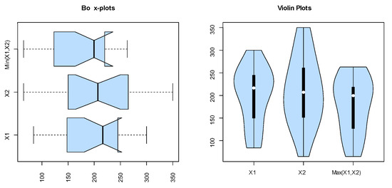
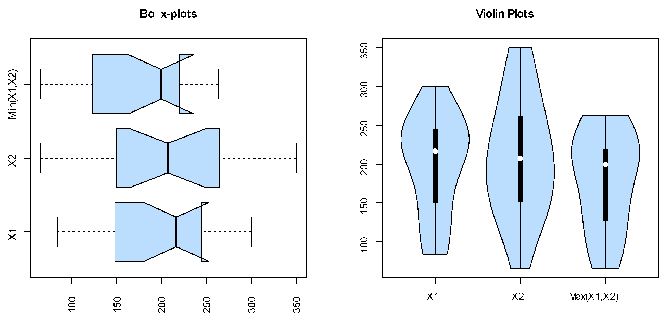
Figure 15.
The box and violin plots for the marginals of dataset II.
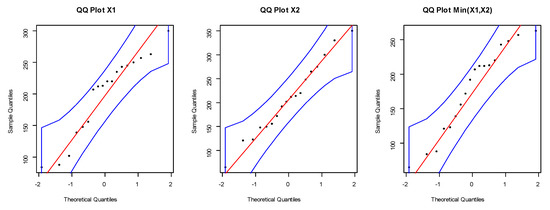
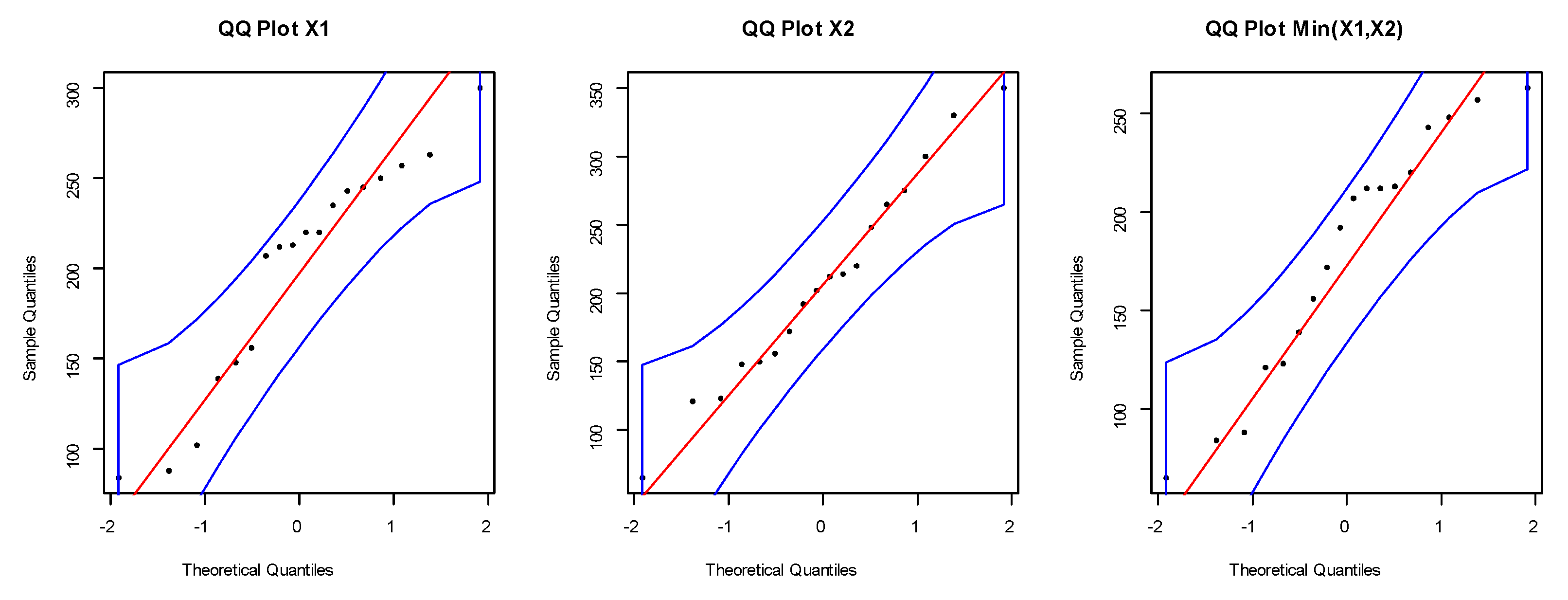
Figure 16.
The QQ plots for the marginals of dataset II.
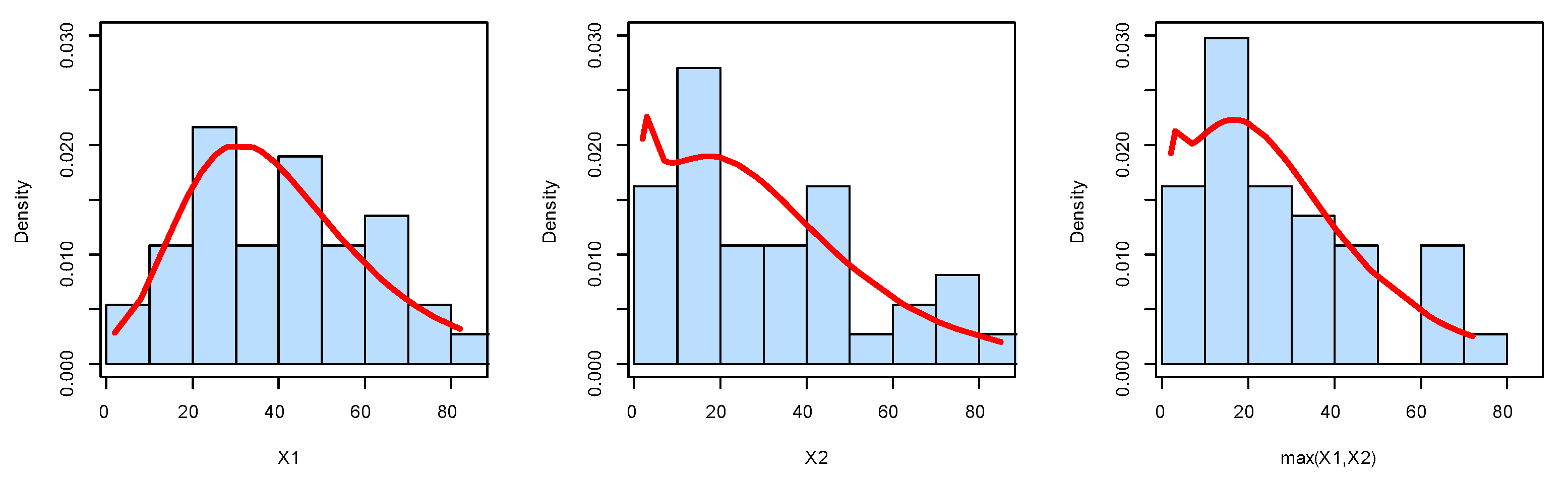
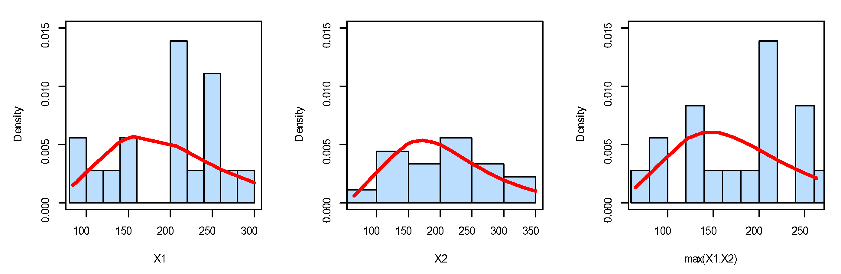
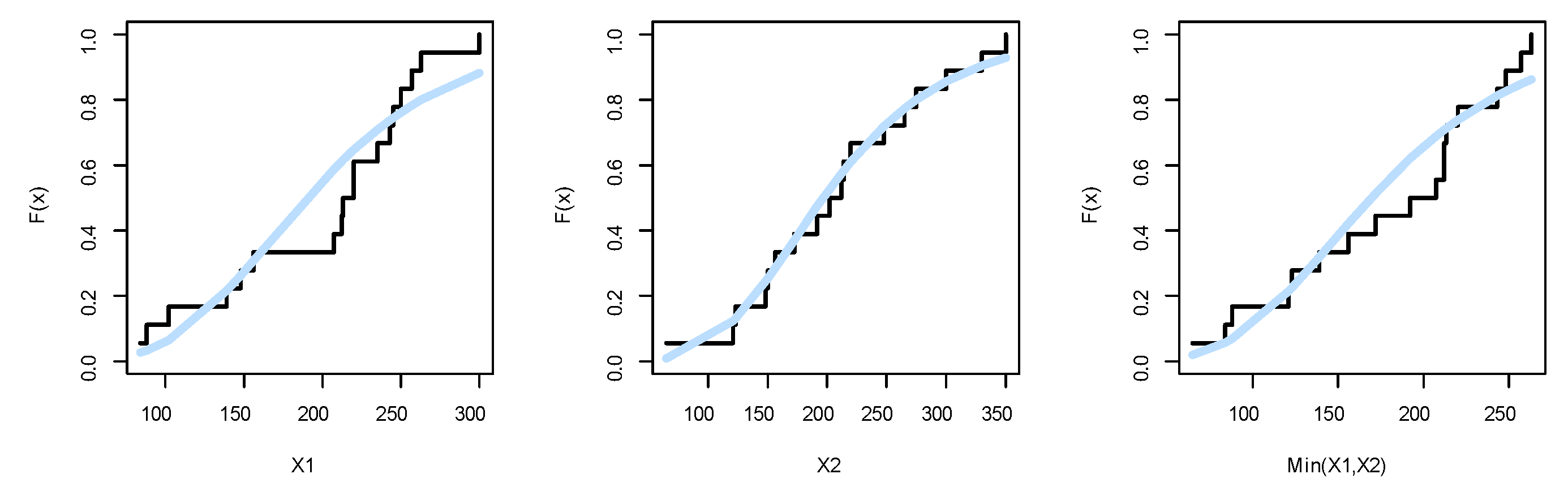
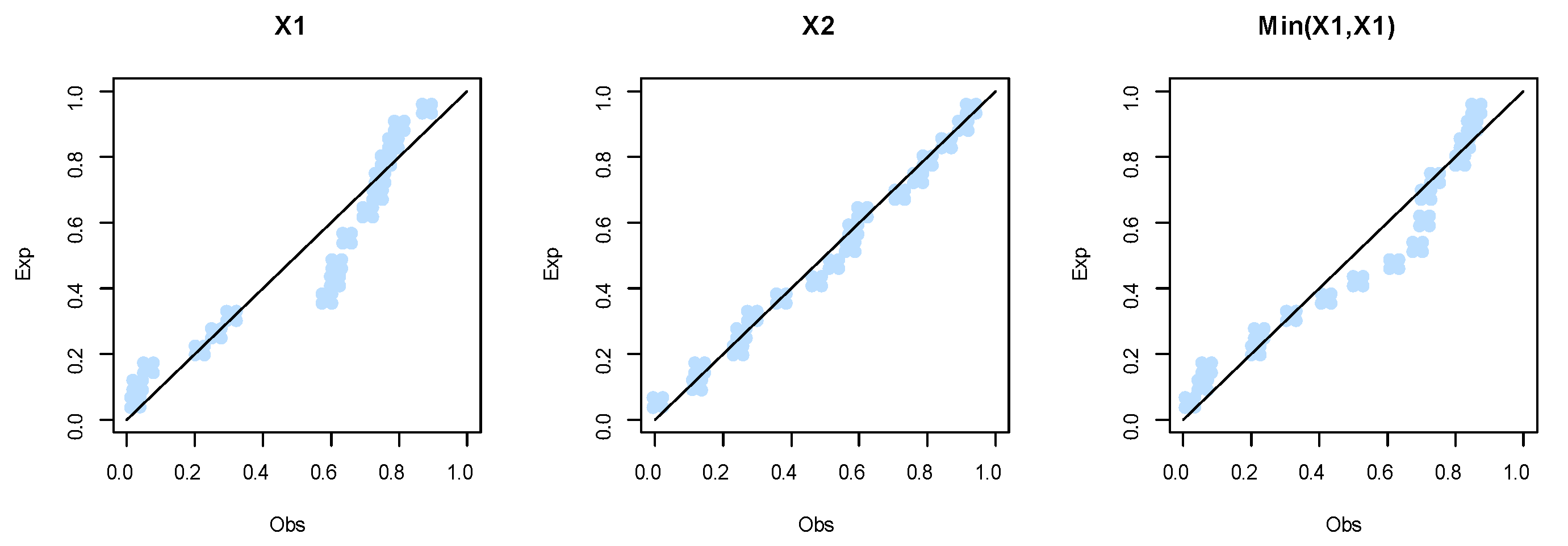
First, we fit the marginals , , and min() separately on the motor data. The MLEs of the parameters for , , and min() are (2.9254, 0.0155, 12.9952), (2.3991, 0.0145, 11.8768), and (2.6118, 0.0164, 10.9977), respectively. The , K-S and its p-value for the marginals , , and min() can be listed as (102.0146, 0.2566, 0.1867), (103.6497, 0.0892, 0.9961), and (101.1782, 0.1908, 0.5291), respectively. According to p-values, it is noted that the BEIFWE distribution fits the data for the marginals. Figure 17, Figure 18 and Figure 19 show the fitted PDFs, estimated CDF, and PP plots for the marginals , , and min(), which prove our results.
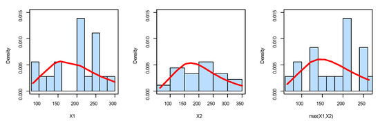
Figure 17.
The fitted PDF plots for the marginals of dataset II.
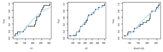
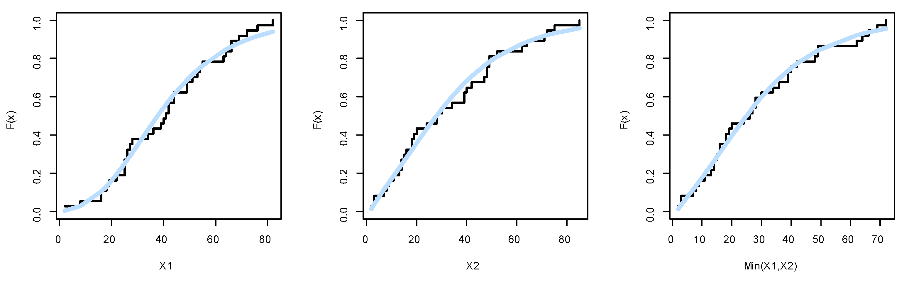
Figure 18.
The estimated CDFs plots for the marginals of dataset II.
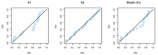
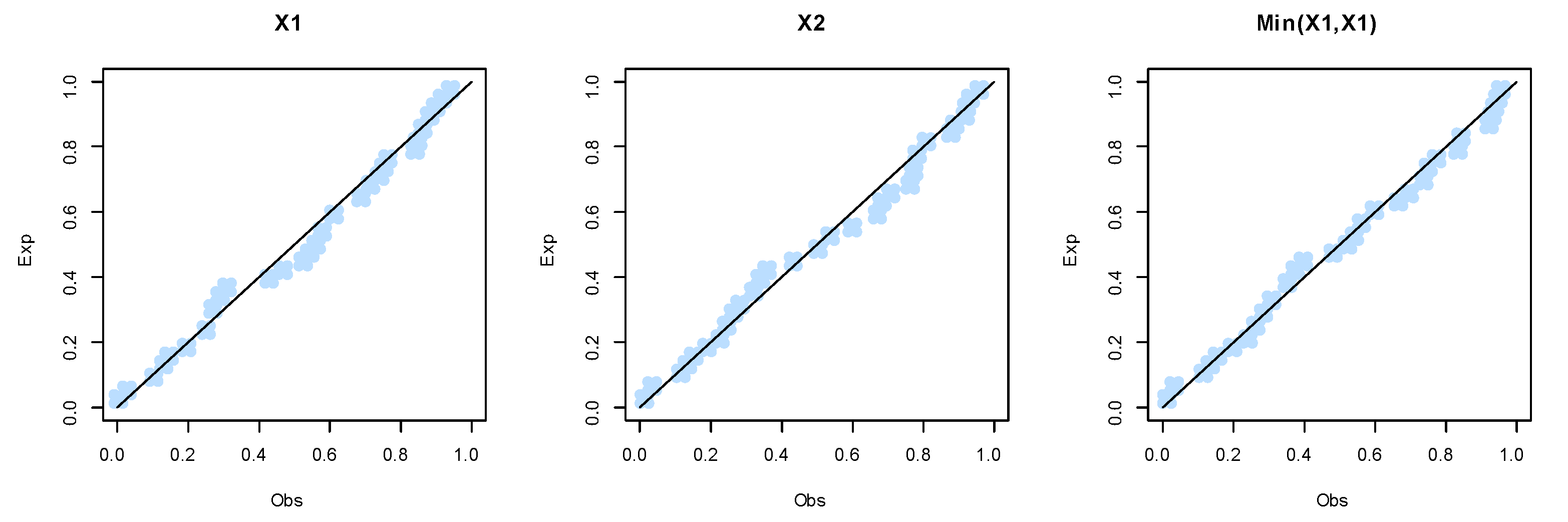
Figure 19.
The fitted PP plots for the marginals of dataset II.
Now, we fit the BEIFWE model on dataset II. In the enclosed Table 3 and Table 4, we report the MLEs, , AIC, CAIC, BIC, and HQIC values for the tested models.
Table 3.
The MLEs for the competitive distributions’ parameters of dataset II.
Table 4.
The goodness-of-fit results for the competitive distributions of dataset II.
Based on the empirical results, it was found that the BEIFWE model fits the data better than the other competitive distributions.
7. Conclusions and Future Work
In this article, a novel bivariate probabilistic distribution was presented and discussed based on the Marshall–Olkin shock model. The proposed bivariate model can be used as a probabilistic tool for discussing and analyzing only the common continuous random variables. After introducing the mathematical structure of the bivariate distribution, some of its statistical properties were derived. The new model revealed interesting features; for instance, the joint PDF can be used as a statistical approach to model different shapes of data, including symmetric and asymmetric forms under various kinds of dispersion; detailed HRFs can be applied to discuss and evaluate different forms of failure rates; and it can be utilized quite conveniently if there are ties in the data. Based on a simulation study, the maximum likelihood technique was applied to estimate the model parameters. Finally, two real datasets were analyzed to demonstrate the ability and observation of the presented bivariate model, and it was found that the presented model provided a better fit than competitive bivariate distributions. As a future study, a bivariate fuzzy time series will be discussed for forecasting. Moreover, the Bayesian technique will be discussed under different approaches, including a priori and non-information, to model complete, censored, and recorded data.
Author Contributions
Conceptualization, M.E.-M. and M.S.E.; methodology, M.H.T. and M.A.; software, M.E.-M. and M.S.E.; validation, R.E.-D., A.A.-B. and H.A.; formal analysis, M.S.E. and M.H.T.; investigation, M.A. and H.A.; resources, R.E.-D. and A.A.-B.; data curation, M.S.E.; writing—original draft preparation, M.E.-M. and M.S.E.; writing—review and editing, M.S.E. and M.H.T.; visualization, M.E.-M.; supervision, R.E.-D. and H.A. All authors have read and agreed to the published version of the manuscript.
Funding
This paper has not received any funding.
Data Availability Statement
The datasets are available in the paper.
Acknowledgments
This study is supported via funding from Prince Sattam bin Abdulaziz University, project number (PSAU/2023/R/1444).
Conflicts of Interest
The authors declare no conflict of interest.
References
- Marshall, A.W.; Olkin, I.A. A multivariate exponential distribution. J. Am. Stat. Assoc. 1967, 62, 30–44. [Google Scholar] [CrossRef]
- Domma, F. Some properties of the bivariate Burr type III distribution. Statistics 2010, 44, 203–215. [Google Scholar] [CrossRef]
- Sarhan, A.M.; Hamilton, D.C.; Smith, B.; Kundu, D. The bivariate generalized linear failure rate distribution and its multivariate extension. Comput. Stat. Data Anal. 2011, 55, 644–654. [Google Scholar] [CrossRef]
- Barreto-Souza, W.; Lemonte, A.J. Bivariate Kumaraswamy distribution: Properties and a new method to generate bivariate classes. Statistics 2013, 47, 1321–1342. [Google Scholar] [CrossRef]
- Kundu, D.; Gupta, A.K. On bivariate Weibull-geometric distribution. J. Multivar. Anal. 2014, 123, 19–29. [Google Scholar] [CrossRef]
- Shahen, H.S.; El-Bassiouny, A.H.; Abouhawwash, M. Bivariate exponentiated modified weibull distribution. J. Stat. Probab. 2019, 8, 27–39. [Google Scholar] [CrossRef]
- Eliwa, M.S.; El-Morshedy, M. Bivariate Gumbel-G family of distributions: Statistical properties, Bayesian and non-Bayesian estimation with application. Ann. Data Sci. 2019, 6, 39–60. [Google Scholar] [CrossRef]
- Eliwa, M.S.; El-Morshedy, M. Bivariate odd Weibull-G family of distributions: Properties, Bayesian and non-Bayesian estimation with bootstrap confidence intervals and application. J. Taibah Univ. Sci. 2020, 14, 331–345. [Google Scholar] [CrossRef]
- Franco, M.; Vivo, J.M.; Kundu, D. A generator of bivariate distributions: Properties, estimation, and applications. Mathematics 2020, 8, 1776. [Google Scholar] [CrossRef]
- Tahir, M.H.; Hussain, M.A.; Cordeiro, G.M.; El-Morshedy, M.; Eliwa, M.S. A new Kumaraswamy generalized family of distributions with properties, applications, and bivariate extension. Mathematics 2020, 8, 1989. [Google Scholar] [CrossRef]
- El-Morshedy, M.; Tahir, M.H.; Hussain, M.A.; Al-Bossly, A.; Eliwa, M.S. A new flexible univariate and bivariate family of distributions for unit interval (0, 1). Symmetry 2022, 14, 1040. [Google Scholar] [CrossRef]
- Kundu, D. Bivariate Semi-parametric Singular Family of Distributions and its Applications. Sankhya B 2022, 84, 846–872. [Google Scholar] [CrossRef]
- El-Morshedy, M.; El-Bassiouny, A.H.; El-Gohary, A. Exponentiated inverse flexible Weibull extension distribution. J. Stat. Appl. Probab. 2017, 6, 169–183. [Google Scholar] [CrossRef]
- Basu, A.P. Bivariate failure rate. J. Am. Stat. Assoc. 1971, 66, 103–104. [Google Scholar] [CrossRef]
- Bismi, G. Bivariate Burr Distributions. Ph.D. Thesis, Cochin University of Science and Technology, Kerala, India, 2005. [Google Scholar]
- Al-Khedhairi, A.; El-Gohary, A. A new class of bivariate Gompertz distributions and its mixture. Int. J. Math. Anal. 2008, 2, 235–253. [Google Scholar]
- El-Morshedy, M.; Alhussain, Z.A.; Atta, D.; Almetwally, E.M.; Eliwa, M.S. Bivariate Burr X generator of distributions: Properties and estimation methods with applications to complete and type-II censored samples. Mathematics 2020, 8, 264. [Google Scholar] [CrossRef]
- Kundu, D.; Gupta, R.D. Bivariate generalized exponential distribution. J. Multivar. Anal. 2009, 100, 581–593. [Google Scholar] [CrossRef]
- Jose, K.K.; Ristić, M.M.; Joseph, A. Marshall–Olkin bivariate Weibull distributions and processes. Stat. Pap. 2011, 52, 789–798. [Google Scholar] [CrossRef]
- El-Bassiouny, A.H.; El-Damcese, M.; Abdelfattah, M.; Eliwa, M.S. Bivariate exponentaited generalized Weibull-Gompertz distribution. J. Appl. Probab. Stat. 2016, 11, 25–46. [Google Scholar]
- El-Gohary, A.; HEl-Bassiouny, A.; El-Morshedy, M. Bivariate exponentiated modified Weibull extension distribution. J. Stat. Appl. Probab. 2016, 5, 67–78. [Google Scholar] [CrossRef]
- Hanagal, D.D. Weibull extension of bivariate exponential regression model with gamma frailty for survival data. Econ. Qual. Control 2006, 21, 261–270. [Google Scholar] [CrossRef]
- Meintanis, S.G. Test of fit for Marshall-Olkin distributions with applications. J. Stat. Plan. Inference 2007, 137, 3954–3963. [Google Scholar] [CrossRef]
- Relia Softs, R.; Staff, D. Using QALT models to analyze system configurations with load sharing. Reliab. Edge 2002, 3, 1–4. [Google Scholar]


Disclaimer/Publisher’s Note: The statements, opinions and data contained in all publications are solely those of the individual author(s) and contributor(s) and not of MDPI and/or the editor(s). MDPI and/or the editor(s) disclaim responsibility for any injury to people or property resulting from any ideas, methods, instructions or products referred to in the content. |
© 2023 by the authors. Licensee MDPI, Basel, Switzerland. This article is an open access article distributed under the terms and conditions of the Creative Commons Attribution (CC BY) license (https://creativecommons.org/licenses/by/4.0/).