Article

Two-Step Self-Calibration of LiDAR-GPS/IMU Based on Hand-Eye Method

1
State Key Laboratory of Advanced Design and Manufacturing for Vehicle Body, Hunan University, Changsha 410082, China
2
School of Physics and Telecommunication Engineering, South China Normal University, Guangzhou 510006, China
3
The Autocity (Shenzhen) Autonomous Driving Co., Ltd., Shenzhen 518000, China
*
Author to whom correspondence should be addressed.
These authors contributed equally to this work.
Symmetry 2023, 15(2), 254; https://doi.org/10.3390/sym15020254
Submission received: 21 December 2022 / Revised: 11 January 2023 / Accepted: 13 January 2023 / Published: 17 January 2023
(This article belongs to the Special Issue Recent Progress in Robot Control Systems: Theory and Applications)

Abstract

:
Multi-line LiDAR and GPS/IMU are widely used in autonomous driving and robotics, such as simultaneous localization and mapping (SLAM). Calibrating the extrinsic parameters of each sensor is a necessary condition for multi-sensor fusion. The calibration of each sensor directly affects the accurate positioning control and perception performance of the vehicle. Through the algorithm, accurate extrinsic parameters and a symmetric covariance matrix of extrinsic parameters can be obtained as a measure of the confidence of the extrinsic parameters. As for the calibration of LiDAR-GPS/IMU, many calibration methods require specific vehicle motion or manual calibration marking scenes to ensure good constraint of the problem, resulting in high costs and a low degree of automation. To solve this problem, we propose a new two-step self-calibration method, which includes extrinsic parameter initialization and refinement. The initialization part decouples the extrinsic parameters from the rotation and translation part, first calculating the reliable initial rotation through the rotation constraints, then calculating the initial translation after obtaining a reliable initial rotation, and eliminating the accumulated drift of LiDAR odometry by loop closure to complete the map construction. In the refinement part, the LiDAR odometry is obtained through scan-to-map registration and is tightly coupled with the IMU. The constraints of the absolute pose in the map refined the extrinsic parameters. Our method is validated in the simulation and real environments, and the results show that the proposed method has high accuracy and robustness.

1. Introduction

In autonomous driving and robotics, commonly used sensors are LiDAR, camera, and GPS/IMU. The LiDAR market has broad prospects. It is predicted that by 2025, China’s LiDAR market will be close to USD 2.175 billion (equal to CNY 15 billion), and the global market will be close to USD 4.35 billion (equal to CYN 30 billion). By 2030, China’s LiDAR market will be close to USD 5.075 billion (equal to CYN 35 billion), and the global market will be close to USD 9.425 billion (equal to CYN 65 billion). The annual growth rate of the global market will reach 48.3% (http://www.evinchina.com/newsshow-2094.html, accessed on 2 January 2023). The annual growth rate of vehicle camera modules from 2018 to 2023 is about 15.8%. It is estimated that the annual sales in 2023 will reach USD 5.8 billion (about CYN 39.44 billion), of which robots and cars will account for 75% (https://www.yoojia.com/article/10096726019901689110.html, accessed on 2 January 2023). GPS/IMU is a comprehensive system combining inertial measurement unit (IMU) and global positioning system (GPS), which can provide centimeter-level absolute localization accuracy. A single IMU can only offer a relatively accurate motion estimation in a short time, which depends on the hardware performance of the IMU. The localization error increases rapidly with time. LiDAR (light detection and ranging) is the most critical ranging sensor, which can estimate the relative motion of vehicles in real-time through point cloud registration. LiDAR’s ranging calculation is complex and often needs to be accelerated in a parallel settlement [1], and due to the high cost, FGPA is used as a part of the data processing module to reduce costs [2]. The SLAM based on LiDAR will degenerate where the geometric feature information is sparse. The camera projects the three-dimensional scene onto the two-dimensional image, through which we can obtain visual odometry. However, the visual odometry has scale ambiguity, and the image is also affected by the exposure rate and the light. In order to integrate the advantages of the sensors to achieve better robustness, many tasks need more than one kind of sensor. Multi-sensor fusion has become a trend [3,4,5,6,7,8]. The study in [3] proposes a pipeline inspection and retrofitting based on LiDAR and camera fusion for an AR system. In [4], for the loss of visual feature tracking of mobile robots, a feature matching method is designed based on a camera and IMU to improve robustness. Efficiently fusing different attributes of the environment captured by the two sensors facilitates a reliable and consistent perception of the environment. In [5], a method for estimating the distance between an autonomous vehicle and other vehicles, objects, and signboards on its path using the accurate fusion of LiDAR and camera is proposed. It can be seen that many tasks tend to use multi-sensor fusion to complete the task. However, since the coordinate systems of the data collected by each sensor are different, we need to unify the coordinate systems of different sensors. This requires different types of data collected by sensors to calibrate the intrinsic parameters of a single sensor and the extrinsic parameters of multiple sensors. For example, Refs. [9,10,11,12] are calibration works about multi-LiDAR extrinsic parameters. Refs. [13,14,15] are calibration works about LiDAR-camera extrinsic parameters. Refs. [16,17,18] are calibration works about LiDAR-IMU extrinsic parameters. There are few calibration works about LiDAR-GPS/IMU extrinsic parameters. The calibration of LiDAR-GPS/IMU is to complete the calibration of extrinsic parameters of LiDAR and IMU rotation and LiDAR and GPS translation.
Since the intrinsic parameters of IMU and LiDAR are usually provided by the manufacturer at the factory, we mainly solve the calibration of extrinsic parameters between LiDAR and GPS/IMU. At present, there are many challenges in the calibration of extrinsic parameters of LiDAR and GPS/IMU. For example, the movement of the vehicle in automatic driving is not like the movement of the robot arm. The movement of the vehicle is mainly the plane movement of three degrees of freedom, which has fewer constraints on the other three degrees of freedom, so the error of the other three degrees of freedom is relatively large. Due to the large difference in the measurement principle between radar and GPS/IMU, to detect the same object in different sensors for calibrating extrinsic parameters between them, many calibration methods require specific vehicle operation and manual calibration marking scenes, resulting in high cost and low degree of automation.
The motion-based method is the primary method for calibration between LiDAR and GPS/IMU. Geiger et al. [19] proposed to use a hand–eye calibration method to constrain GPS/IMU odometry and obtain LiDAR odometry through point-plane registration. However, it does not have an initial extrinsic parameter calculation, so its accuracy depends on the high-precision registration of the LiDAR odometry. Hand–eye calibration utilizes the hand-eye model proposed in the field of robotics. It is used to solve the rigid transformation between the manipulator and the camera rigidly mounted above, and this problem can be extended to solve the problem of relatively rigid transformation between any two sensors [20,21]. Therefore, we can also use it to solve the rigid transformation between LiDAR and GPS/IMU. Hand–eye calibration mainly solves the equation AX = XB, where A and B are the odometry of two different sensors, respectively, and X is the extrinsic parameters between the two sensors. In [22], the ground is used to solve the Z-axis translation, roll, and pitch transformation, and then the three-dimensional problem is converted into a two-dimensional problem. The remaining three degrees of freedom are estimated by hand–eye calibration. It can be regarded as taking the three degrees of freedom optimized on the ground as the initial value and then performing hand–eye calibration. The initial value calculation is too simple and rough, there are manual operation errors, and the obtained accuracy is relatively low. Baidu’s open-source Apollo project divides the calibration process into two steps. First, calculate the initial calibration parameters through the trajectory and then refine the calibration parameters through the feature-based method. Our calibration method shares the same idea, which is to complete the calibration parameters from the coarse to the fine, but the details of the method implementation are different. We adopt more strategies, such as loop closure detection and tight coupling strategies, so the accuracy and robustness are relatively better. In [23], in order to solve the problem of missing constraints caused by the plane motion of vehicle motion, large-range and small-range trajectories are used to solve the extrinsic parameters of rotation and translation, respectively. However, large-range trajectory recording requires a large labor cost and is demanding; therefore, the method is not universal. The advantages and disadvantages of related work are shown in Table 1.
This paper proposes a new two-step self-calibration method, which includes extrinsic parameters initialization and refinement. The initialization part decouples the extrinsic parameters from the rotation and translation part by first calculating the reliable initial rotation through the rotation constraints, then calculating the initial translation after obtaining a reliable initial rotation, and eliminating the accumulated drift of LiDAR odometry by loop closure to complete the map construction. In the refinement part, the LiDAR odometry is obtained through scan-to-map registration and is tightly coupled with the IMU. The constraints of the absolute pose in the map refined the extrinsic parameters. The main contributions of our work can be summarized as follows:
  • A new LiDAR and GPS/IMU calibration system can be calibrated daily in an open natural environment and has good universality.
  • Like the common localization problem, we divide the calibration problem into two steps and adopt the idea from coarse to fine to make the extrinsic parameters have better robustness and accuracy and effectively eliminate the influence of accumulated drift on the extrinsic parameters.
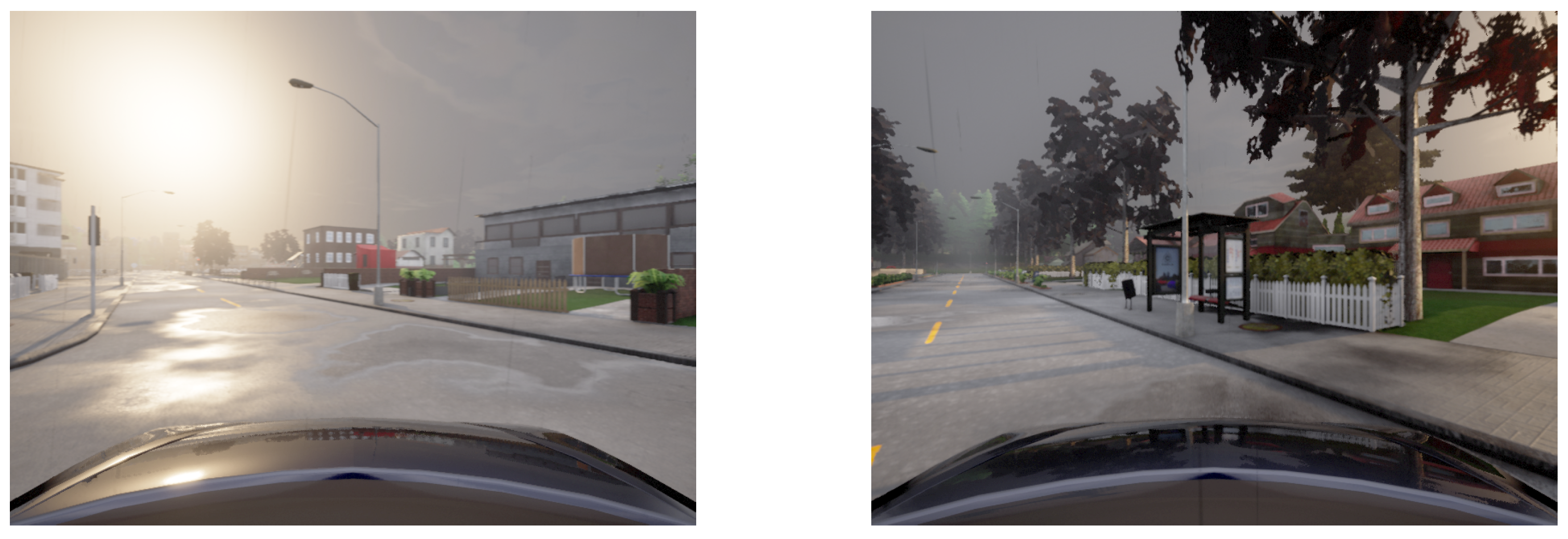
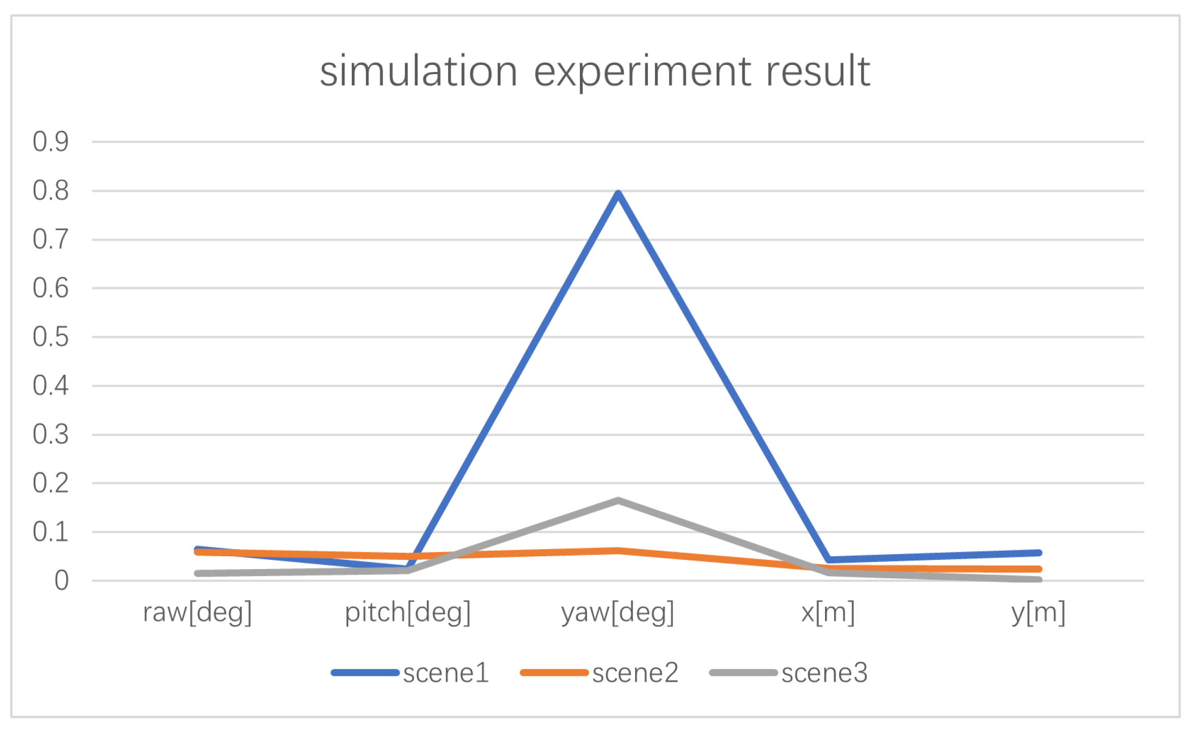
  • The proposed calibration system is verified in both a simulation environment and a real environment.
The rest of the paper is organized as follows: Section 2 is an overview of the system, which describes the core calibration algorithm of the LiDAR-GPS/IMU calibration system, which is divided into two parts to introduce our proposed algorithm and provide a detailed introduction to the algorithm. Section 3 is the experimental results of the simulation and real environment. Section 4 is the summary of this paper and future work. Table 2 is all the abbreviations used in this article.

2. Methods

This section introduces the architecture of the proposed LiDAR-GPS/IMU calibration system, as shown in Figure 1. The system is mainly divided into two parts: parameter initialization and parameter refinement. In the parameter initialization part, the feature-based LiDAR odometry and the interpolated GPS/IMU relative pose were used to construct the hand–eye calibration problem to solve the initial extrinsic parameters and construct the map. In the parameter refinement part, LiDAR and IMU are tightly coupled by the initial extrinsic parameters, and the extrinsic parameters were refined through the constraints of the absolute pose in the map.
The core of the extrinsic parameter initialization is a hand–eye calibration algorithm. When the vehicle is in motion, Figure 2 shows the relationship between relative and absolute pose during hand–eye calibration of LiDAR and GPS/IMU, where the { W } is the first frame of the GPS/IMU, and the { L k } and { I k } represent the k th frame of the LiDAR and the GPS/IMU frame obtained by interpolation at this time, respectively. T I k W is the absolute pose of { I k } relative to { W } . T I k + 1 I k is the relative pose from { I k + 1 } to { I k } . T L k + 1 L k is the relative pose from { L k + 1 } to { L k } . It is easy to see from Figure 2 that we have two ways to obtain the relative pose from { L k + 1 } to { I k } , so we can obtain the formula as follows:
T I k + 1 I k T L I = T L I T L k + 1 L k
Equation (1) constitutes the equation AX = XB for hand–eye calibration. The principle of hand–eye calibration will be introduced in detail below.

2.1. Hand–Eye Calibration

Equation (1) is usually decoupled into two parts according to [24]: rotation and translation. As the vehicle moves, the following equation holds for any k:
R I k + 1 I k R L I = R L I R L k + 1 L k
R I k + 1 I k I 3 t L I = R L I t L k + 1 L k t I k + 1 I k

2.1.1. Extrinsic Rotation

Equation (2) is expressed by a quaternion as follows:
q I k + 1 I k q L I = q L I q L K + 1 L k q I k + 1 I k L q I k + 1 I k R ) q L I = Q k + 1 k q L I
where ⊗ is the quaternion multiplication operator, and q I k + 1 I k L and q I k + 1 I k R are the matrix representation of the left and right quaternion multiplication, respectively [25]. After stacking measurements at different times, we obtain an over-determined equation as follows:
w 2 1 · Q 2 1 w k + 1 k · Q k + 1 k 4 K × 4 q L I = Q K q L I = 0 4 K × 4
where K is the number of rotation pairs of the over-determined equation, and w k + 1 k is the robust weight to better handle outliers. The angle of the current rotation pair difference in the angular axis is calculated by Equation (4) and taken as the parameters of Huber loss, whose derivative is the weight:
w k + 1 k = ρ ( θ ) , θ = 2 arccos q w q = ( q I k + 1 I k q L I ) * q L I q L K + 1 L k
where ρ ( ) is Huber loss, q w is the real part of the quaternion q , and ( ) * means taking the inverse of the quaternion. We use SVD to solve the over-determined Equation (5), whose closed solution is the right unit singular vector corresponding to the minimum singular value. Meanwhile, according to [26], to ensure sufficient rotation constraints, we need to ensure that the second smallest singular value is large enough, which needs to be larger than the artificial threshold. With the rapid increase of Q k + 1 k , the priority queue is used to remove the constraint with the smallest rotation. Until the second smallest singular value exceeds the threshold, we can obtain a reliable initial extrinsic rotation.

2.1.2. Extrinsic Translation

When the extrinsic rotation R ^ L I is obtained, translation can be solved by the least square approach according to Equation (3).
R I 2 I 1 I 3 R I k + 1 I k I 3 3 K × 3 t L I = R ^ L I t L 2 L 1 t I 2 I 1 R ^ L I t L k + 1 L k t I k + 1 I k 3 K × 1
However, the vehicle motion is usually a three degrees of freedom plane motion, so the translation of the z axis, t z , is not reliable. At the same time, since the acceleration of IMU is coupled with gravity, it is related to rotation, so it is also not reliable to calculate the initial translation value through the initial rotation. We can make the plane assumption as [10] and rewrite Equation (7) as follows:
R k + 1 t x t y cos ( γ ) sin ( γ ) sin ( γ ) cos ( γ ) t k + 1 1 = t k + 1 2
Equation (8) is the plane motion constraint generated by the k + 1 th relative pose, where γ is the yaw rotation, t x and t y are the translation of the x and y axes, respectively, R k + 1 is the 2x2 block matrix in the upper left corner of R I k + 1 I k I 3 , and t k + 1 1 and t k + 1 2 are the first two elements of the column vectors R L I t L k + 1 L k and t I k + 1 I k , respectively.
Equation (8) can be rewritten in the form of the matrix equation AX = b:
R k + 1 J A k + 1 t x t y cos ( γ ) sin ( γ ) = t k + 1 2
where J = t k + 1 1 1 t k + 1 1 2 t k + 1 1 2 t k + 1 1 1 , t k + 1 1 i denotes the i th element of the column vector t k + 1 1 . As in Equation (5), by stacking measurements at different times according to Equation (9), we can obtain the final matrix equation AX = b, which can be solved by the least-squares approach:
A 2 A K + 1 A 2 K × 4 t x t y cos ( γ ) sin ( γ ) x 4 × 1 = t 2 2 t K + 1 2 b 2 K × 1
The obtained yaw rotation, according to Equation (10), is fused with the original calculated extrinsic rotation R ^ L I to obtain the new initial rotation. We can manually measure the value of the extrinsic parameters about the z-axis. Suppose the calculated translation of the extrinsic parameters about the Z-axis differs too much from the measured value. In that case, we can set the translation of the Z-axis to the measured value and refine it through the absolute pose constraint in the refinement part; see Section 2.2.2.

2.2. Methods

This section details the procedure for calculating the initial values of extrinsic parameters by GPS/IMU measurements and LiDAR measurements. First, the GPS/IMU measurements were interpolated against the LiDAR timestamp; then, the LiDAR odometry was estimated as in [27]. The extrinsic parameters were initialized by hand–eye calibration; see Section 2.1. We integrate loop closure into the system by using a factor graph and completing the map construction. Then, we tightly coupled LiDAR and IMU through the initially obtained extrinsic parameters, obtained the LiDAR odometry through scan-to-map feature-based registration, and refined the extrinsic parameters by constructing the constraints of the extrinsic parameters through the obtained absolute pose.

2.2.1. Extrinsic Parameters Initialization

As for LiDAR odometry, there are two methods to calculate the relative transformation of two consecutive frames: 1. based on direct matching, such as ICP [28] and GICP [29], 2. feature-based methods, such as LOAM [27], do not need to calculate all the point clouds but only need to calculate representative points, which not only improves accuracy but also reduces computing efficiency. We use the feature-based method in [30] to obtain the LiDAR odometry.
However, since there are no extrinsic parameters between the LiDAR and IMU, we cannot use the IMU pre-integration as the guess pose of the LiDAR odometry as in [30]. Because offline calibration does not require real-time performance like SLAM, we can add more constraints to make the estimated relative motion more accurate. We first need to compute a predicted pose to prevent the optimization algorithm from converging to a local optimum. With the increase in time, the registration between consecutive frames tends to have a larger drift on the Z-axis than other axes. Therefore, we first use the constant velocity model as the predicted pose and then extract the ground points and calculate the centroid of the ground point to optimize roll, pitch angle, and z-translation, respectively. Since LiDAR is basically installed horizontally, we first extract ground points using geometric features in [31], and then filter the outliers by RANSAC so that the ground points obtained can reach a high accuracy and the guess pose is relatively accurate.
When we obtain the latest scans of the raw LiDAR point cloud, firstly, we de-skew the point cloud to the moment of the first LiDAR point by guess pose and project the skewed point cloud into the range image according to the resolution. We extract the two feature points, edge feature and planar feature points, through the curvature. We distribute the feature points uniformly and remove the unstable feature points as [27]. We denote F k = F k e , F k p as all feature points of k th LiDAR point cloud, and F k e and F k p are denoted as edge feature points and planar feature points, respectively. We can obtain the distances of point-to-line and point-to-plane through the following:
d e k = p k + 1 e p ¯ k , 2 e × p k + 1 e p ¯ k , 1 e p ¯ k , 1 e p ¯ k , 2 e
n = p ¯ k , 1 p p ¯ k , 2 p × p ¯ k , 1 p p ¯ k , 3 p
d p k = p k + 1 p p ¯ k , 1 p · n n
where p k + 1 e F k + 1 e , p k + 1 p F k + 1 p . F k + 1 = F k + 1 e , F k + 1 p is the feature points de-skewed to the first point of the current point cloud. p ¯ k , 1 e , p ¯ k , 2 e are the two edge feature points of F ¯ k e corresponding to p k + 1 e . p ¯ k , 1 p , p ¯ k , 2 p , p ¯ k , 3 p are the three planer feature points of F ¯ k p corresponding to p k + 1 p . F ¯ k = F ¯ k e , F ¯ k p is the feature points de-skewed to the last point of the previous point cloud. The moment of the last point of the previous point cloud is equal to the moment of the first point of the current point cloud, so the edge feature points at the same moment are on the same line, and the planner points are on the same surface. Thus, we can obtain the constraint of Equations (11)–(13) and use point-to-line and point-to-surface distances as cost functions. The relative pose can be calculated by minimizing the cost function by using the Levenberg–Marquardt algorithm. The LiDAR odometry algorithm is shown in Algorithm 1.
Algorithm 1 LiDAR Odometry.
Input: 
F ¯ k = F ¯ k e , F ¯ k p , F k + 1 = F k + 1 e , F k + 1 p , T L k W from the last recursion
Output: 
F ¯ k + 1 = F ¯ k + 1 e , F ¯ k + 1 p , T L k + 1 W
  1:
Through the constant velocity model, guess pose T L k + 1 W is calculated from T L k W
  2:
for each edge point in F k + 1  do
  3:
    Extracting ground points through geometric features and RANSAC
  4:
end for
  5:
Calculate the three degrees of freedom z-translation, roll, and pitch through ground point optimization to obtain a new guess pose T L k + 1 W .
  6:
De-skew the point cloud F k + 1 to the moment of the first LiDAR point by guess pose. Detect edge points and planar points in F k + 1
  7:
for a number of iterations do
  8:
    for each edge point in F k + 1 e  do
  9:
   Find an edge line as the correspondence, then compute point to line distance based on (11)
 10:
    end for
 11:
    for each edge point in F k + 1 e  do
 12:
   Find a planar patch as the correspondence, then compute point to plane distance based on (13)
 13:
    end for
 14:
    Using distance as a cost function for nonlinear optimization, update T L k + 1 W
 15:
    if the nonlinear optimization converges then
 16:
   Break
 17:
    end if
 18:
end for
 19:
Reproject F k + 1 to the moment of the last LiDAR point according to T L k + 1 W to get F ¯ k + 1
 20:
return T L k + 1 W , F ¯ k + 1
After completing the registration between two consecutive frames, we optimize the estimated pose again through scan-to-map point cloud registration. We obtain the keyframe through the relative pose transformation amount greater than the threshold value that is considered to be set and save it. The local point cloud used for the current point cloud registration is obtained through the following two methods: 1. It is formed by superimposing several keyframes adjacent in time. 2. It is formed by superimposing several keyframes adjacent in position. The search for adjacent positions uses a KD-tree and adds the position of each keyframe as a point to the KD-tree, and then the keyframes with adjacent positions are obtained through the nearest neighbor search of the KD-tree. In order to reduce the drift of cumulative errors, we combined the obtained relative pose with z-translation, roll, and pitch angle obtained by ground point optimization to make the relative pose more accurate and robust.
After obtaining the relative pose of LiDAR, the initial calibration parameters can be obtained by hand–eye calibration through the relative pose constraints of the LiDAR odometry and the relative pose constraints of the interpolated GPS/IMU data; see Section 2.1. We denote q L K + 1 L k , t L K + 1 L k and q I K + 1 I k , t I K + 1 I k as the relative pose constraint pair of LiDAR data and GPS/IMU data, respectively. We can construct the following cost function with extrinsic parameters:
min q I L , t I L k N ( q I k + 1 I k q L I ) * q L I q L K + 1 L k x y z 2 + k N R I k + 1 I k I 3 t L I R L I t L k + 1 L k + t I k + 1 I k 2
where x y z represents the imaginary part of the quaternion, and there are a total of N relative pose constraint pairs. If we make a planar assumption, the residuals of the translation part can be constructed by Equation (10). After multiple optimizations, the initial value of the calibration parameters can be obtained. The global consistency map is constructed by a loop closure.

2.2.2. Extrinsic Parameters Refinement

In this section, the process of extrinsic parameter refinement is introduced in detail. First, the absolute pose is obtained through the registration of the global map obtained from Section 2.2.1. The LiDAR odometry and IMU and tightly coupled by the initial extrinsic parameters, and the cost function of the calibration parameters was constructed by the absolute pose. After nonlinear optimization, the refined extrinsic parameters can be obtained.
From Section 2.2.1, we can obtain the initial extrinsic parameters, the global map, and the world frame. The global map is built under the world frame. Since we have the initial extrinsic parameters, we can tightly couple the IMU during the construction of the LiDAR odometry. Firstly, the pre-integration is used to de-skew the LiDAR point cloud and serve as the guess pose of the LiDAR odometry. The bias of the IMU is corrected by the optimized LiDAR odometry based on the factor graph.
First, we obtain the local map by filtering the global map and obtain the LiDAR odometry by registration with the local map, T L k W . Through Figure 3, we can construct constraints with extrinsic parameters through the following formula:
T L k W = T I k W T ^ L I
where T I k W is the GPS/IMU pose corresponding to the current LiDAR timestamp.
As per Section 2, we can also decouple Equation (15) into the rotation part and the translation part to obtain the following two constraints [24]:
q ^ L k W = q I k W q L I , t ^ L k W = t I k W + R I k W t L I .
The construction of the over-determined equation about rotation and translation is the same as Section 2.2.1, but the assumption of plane motion is not required here, the extrinsic translation parameters can be optimized by the absolute pose, directly.
We can refine the extrinsic parameters by constructing the cost function of the absolute pose and extrinsic parameters according to Equation (16):
min q L I , t L I k N ( q L i W ) * q I i W q L I x y z 2 + k N R I k W t L I + t I k W t L k W 2
When the cost function is optimized by L-M optimization, the final precise extrinsic parameters can be obtained when the iteration converges.

3. Results and Discussions

3.1. Validation and Results

In this section, we validate the proposed LiDAR-GPS/IMU calibration system in the simulation and real environments, respectively. The simulation environment adopted the Carla simulation platform and was equipped with the required sensors to record multiple data sets under the empty urban road scene. In the real environment, ouster-128 LiDAR and FDI-integrated navigation systems were used to record corresponding data sets in outdoor road scenes, and CAD assembly drawing was used as the ground truth for comparison and verification. In addition to the above hardware configuration, the software configuration in Table 3 is also required. Data communication was performed through ROS in the Ubuntu operating system, the received LiDAR point cloud was processed through PCL, and nonlinear optimization was performed through Ceres Solver. Upon playing the pre-recorded data set, the system receives LiDAR, GPS, and IMU messages through ROS and obtains the global map and initial extrinsic parameters through the method of extrinsic parameters initialization in Section 2.2.1. After the initialization of the extrinsic parameters is completed, the global map and the initial extrinsic parameters are loaded through the method of refining the extrinsic parameters described in Section 2.2.2 to carry out the refinement operation so that the final result of the experiment can be obtained.

3.1.1. Simulation

As shown in Figure 4, there is the scene diagram built by the Carla simulation platform. Carla [32] is an urban driving simulator and has an ROS interface to support the sensor suite. Carla can be installed through Carla’s official website tutorial. Note that installing Carla requires about 130GB of disk space and at least a 6GB GPU. The vehicle is equipped with LiDAR and GPS/IMU, and the ground truth and noise model size are given through the configuration file. After completing the hardware configuration and setting the configuration file, data sets can be recorded in different scenarios. After comparing the data sets in different scenarios, the experimental data were recorded in Table 4. Figure 5 shows the variation trend of the error values of rotation and translation. Both the rotation part and the translation part can achieve high precision. Regarding the rotation part, the error of raw angle and pitch angle is within 0.1 degrees, the error of yaw angle is relatively large, the error of scene 2 and scene 3 is within 0.2 degrees, and the error of scene 1 is about 0.8 degrees. Regarding the translation part, all errors are within 0.1 m.

3.1.2. Real-World Experiments

We assembled the sensors, as shown in Figure 6, to collect data, respectively, in the outdoor scene. The ouster-128 Lidar outputs the point cloud at a frequency of 10 Hz, and the FDI-integrated navigation system outputs the GPS/IMU measurement at a frequency of 100 Hz. Since there is no ground truth of LiDAR-GPS/IMU in the real scene and there is also a lack of an open source LiDAR-GPS/IMU calibration algorithm, we adopted the truth value provided by CAD assembly drawing for verification and checked the repeatability and correctness of calibration results through many experiments. The experimental results are shown in Table 5. Figure 7 shows the variation trend of the error values of rotation and translation. It can be seen that in the real world, the calibration system we proposed can still reach high accuracy. Regarding the rotation part, the errors of the pitch angles of the three scenes are all within 0.2 degrees, the errors of the raw angles are all within 0.45 degrees, and the errors of the yaw angles are all within 0.6 degrees. Regarding the translation part, all errors are within 0.05 m. Comparing the extrinsic parameters errors obtained in the simulation environment and the real environment, the errors of the pitch angle and the translation part are relatively small, and the errors of the yaw angle are relatively large. The difference is that the error of the raw angle in the real environment is larger than that in the simulation environment.

3.2. Discussions

Many existing calibration methods require specific vehicle movement, such as eight-shaped trajectories, or manually marked scenes so that different sensors can measure the same marker for calibration, resulting in low automation and high labor costs. For multi-sensor fusion, it is crucial to calibrate the extrinsic parameters between sensors. This paper proposes a motion-based self-calibration method, which can complete the calibration in the surrounding natural scenes, such as outdoor roads, urban streets, etc., only requiring the completion of data set recording in advance, and then the extrinsic parameters of LiDAR and GPS/IMU can be obtained through two-step offline calibration. However, due to the plane movement of the vehicle, even if the LiDAR odometry and GPS/IMU odometry are accurately estimated from coarse to fine, the z-axis translation of the extrinsic parameters cannot be well estimated. There is still no good solution to this difficulty. It may be due to the large z-axis drift in the registration algorithm of the LiDAR odometry itself. Perhaps this problem can be better solved by studying a new point cloud registration algorithm.

4. Conclusions and Future Work

In this paper, we propose a self-calibration system of LIDAR-GPS/IMU, which can achieve high-precision calibration of extrinsic parameters between LiDAR and GPS/IMU in natural outdoor scenes. The two-step offline self-calibration method was adopted. Firstly, the initial extrinsic parameters were calibrated by hand-eye calibration, and the accumulated drift was removed by loop closure to complete the map construction. Then, the absolute pose, which was obtained by map-based registration, and extrinsic parameters constructed the cost function, and the extrinsic parameters were refined by the optimization algorithm. It has been verified in many experiments in the simulation environment and real environment and has good robustness and accuracy. Since hand–eye calibration is applicable to any calculation of rigid transformation between two sensors, future work involves the calibration of extrinsic parameters between any two sensors between camera, LiDAR, and GPS/IMU.

Author Contributions

Conceptualization, J.G.; methodology, J.G.; software, Y.Z.; validation, J.G., X.T. and J.C.; formal analysis, J.G.; investigation, J.G. and X.N.; resources, Y.Z.; data curation, J.G.; writing—original draft preparation, J.G. and X.T; writing—review and editing, X.N.; visualization, J.C.; supervision, X.N.; project administration, J.G.; funding acquisition, X.N., J.G., J.C., X.T. and Y.Z. All authors have read and agreed to the published version of the manuscript.

Funding

This research was funded by the Hunan Natural Science Foundation of China, grant number 2020JJ4196, and the Liuzhou Science and Technology Foundation of China, grant number 2021CBA0101.

Institutional Review Board Statement

Not applicable.

Informed Consent Statement

Not applicable.

Data Availability Statement

Not applicable.

Conflicts of Interest

The authors declare no conflict of interest.

References

  1. Mochurad, L.; Kryvinska, N. Parallelization of Finding the Current Coordinates of the Lidar Based on the Genetic Algorithm and OpenMP Technology. Symmetry 2021, 13, 666. [Google Scholar] [CrossRef]
  2. Huang, J.; Ran, S.; Wei, W.; Yu, Q. Digital Integration of LiDAR System Implemented in a Low-Cost FPGA. Symmetry 2022, 14, 1256. [Google Scholar] [CrossRef]
  3. Kumar, G.A.; Patil, A.K.; Kang, T.W.; Chai, Y.H. Sensor Fusion Based Pipeline Inspection for the Augmented Reality System. Symmetry 2019, 11, 1325. [Google Scholar] [CrossRef] [Green Version]
  4. Zhu, D.; Ji, K.; Wu, D.; Liu, S. A Coupled Visual and Inertial Measurement Units Method for Locating and Mapping in Coal Mine Tunnel. Sensors 2022, 22, 7437. [Google Scholar] [CrossRef] [PubMed]
  5. Kumar, G.A.; Lee, J.H.; Hwang, J.; Park, J.; Youn, S.H.; Kwon, S. LiDAR and Camera Fusion Approach for Object Distance Estimation in Self-Driving Vehicles. Symmetry 2020, 12, 324. [Google Scholar] [CrossRef] [Green Version]
  6. Chu, P.M.; Cho, S.; Sim, S.; Kwak, K.; Cho, K. Multimedia System for Real-Time Photorealistic Nonground Modeling of 3D Dynamic Environment for Remote Control System. Symmetry 2018, 10, 83. [Google Scholar] [CrossRef] [Green Version]
  7. Pan, Y.; Xiao, P.; He, Y.; Shao, Z.; Li, Z. MULLS: Versatile LiDAR SLAM via multi-metric linear least square. In Proceedings of the 2021 IEEE International Conference on Robotics and Automation (ICRA), Xi’an, China, 30 May–5 June 2021; pp. 11633–11640. [Google Scholar]
  8. Le, A.V.; Apuroop, K.G.S.; Konduri, S.; Do, H.; Elara, M.R.; Xi, R.C.C.; Wen, R.Y.W.; Vu, M.B.; Duc, P.V.; Tran, M. Multirobot Formation with Sensor Fusion-Based Localization in Unknown Environment. Symmetry 2021, 13, 1788. [Google Scholar] [CrossRef]
  9. Lee, H.; Chung, W. Extrinsic Calibration of Multiple 3D LiDAR Sensors by the Use of Planar Objects. Sensors 2022, 22, 7234. [Google Scholar] [CrossRef] [PubMed]
  10. Jiao, J.; Yu, Y.; Liao, Q.; Ye, H.; Fan, R.; Liu, M. Automatic calibration of multiple 3d lidars in urban environments. In Proceedings of the 2019 IEEE/RSJ International Conference on Intelligent Robots and Systems (IROS), Macau, China, 3–8 November 2019; pp. 15–20. [Google Scholar]
  11. Xue, B.; Jiao, J.; Zhu, Y.; Zhen, L.; Han, D.; Liu, M.; Fan, R. Automatic calibration of dual-LiDARs using two poles stickered with retro-reflective tape. In Proceedings of the 2019 IEEE International Conference on Imaging Systems and Techniques (IST), Abu Dhabi, United Arab Emirates, 9–10 December 2019; pp. 1–6. [Google Scholar]
  12. Zhang, J.; Lyu, Q.; Peng, G.; Wu, Z.; Yan, Q.; Wang, D. LB-L2L-Calib: Accurate and Robust Extrinsic Calibration for Multiple 3D LiDARs with Long Baseline and Large Viewpoint Difference. In Proceedings of the 2022 International Conference on Robotics and Automation (ICRA), Philadelphia, PA, USA, 23–27 May 2022; pp. 926–932. [Google Scholar]
  13. Liu, X.; Yuan, C.; Zhang, F. Targetless Extrinsic Calibration of Multiple Small FoV LiDARs and Cameras using Adaptive Voxelization. IEEE Trans. Instrum. Meas. 2022, 17, 8502612. [Google Scholar] [CrossRef]
  14. Mishra, S.; Osteen, P.R.; Pandey, G.; Saripalli, S. Experimental evaluation of 3d-lidar camera extrinsic calibration. In Proceedings of the 2020 IEEE/RSJ International Conference on Intelligent Robots and Systems (IROS), Las Vegas, NV, USA, 24 October–24 January 2020; pp. 9020–9026. [Google Scholar]
  15. Yuan, K.; Ding, L.; Abdelfattah, M.; Wang, Z.J. LiCaS3: A Simple LiDAR–Camera Self-Supervised Synchronization Method. IEEE Trans. Robot. 2022, 38, 3203–3218. [Google Scholar] [CrossRef]
  16. Li, Y.; Yang, S.; Xiu, X.; Miao, Z. A Spatiotemporal Calibration Algorithm for IMU&LiDAR Navigation System Based on Similarity of Motion Trajectories. Sensors 2022, 22, 7637. [Google Scholar] [PubMed]
  17. Lv, J.; Xu, J.; Hu, K.; Liu, Y.; Zuo, X. Targetless Calibration of LiDAR-IMU System Based on Continuous-time Batch Estimation. In Proceedings of the 2020 IEEE/RSJ International Conference on Intelligent Robots and Systems (IROS), Las Vegas, NV, USA, 24 October–24 January 2020; pp. 9968–9975. [Google Scholar]
  18. Lv, J.; Zuo, X.; Hu, K.; Xu, J.; Huang, G.; Liu, Y. Observability-Aware Intrinsic and Extrinsic Calibration of LiDAR-IMU Systems. IEEE Trans. Robot. 2022, 38, 3734–3753. [Google Scholar] [CrossRef]
  19. Geiger, A.; Lenz, P.; Stiller, C.; Urtasun, R. Vision meets robotics: The kitti dataset. Int. J. Robot. Res. 2013, 32, 1231–1237. [Google Scholar] [CrossRef] [Green Version]
  20. Schneider, S.; Luettel, T.; Wuensche, H.J. Odometry-based online extrinsic sensor calibration. In Proceedings of the 2013 IEEE/RSJ International Conference on Intelligent Robots and Systems, Tokyo, Japan, 3–7 November 2013; pp. 1287–1292. [Google Scholar]
  21. Tsai, R.; Lenz, R. A new technique for fully autonomous and efficient 3D robotics hand/eye calibration. IEEE Trans. Robot. Autom. 1989, 5, 345–358. [Google Scholar] [CrossRef] [Green Version]
  22. Chen, C.; Xiong, G.; Zhang, Z.; Gong, J.; Qi, J.; Wang, C. 3D LiDAR-GPS/IMU Calibration Based on Hand-Eye Calibration Model for Unmanned Vehicle. In Proceedings of the 2020 3rd International Conference on Unmanned Systems (ICUS), Harbin, China, 27–28 November 2020; pp. 337–341. [Google Scholar]
  23. Yuwen, X.; Chen, L.; Yan, F.; Zhang, H.; Tang, J.; Tian, B.; Ai, Y. Improved Vehicle LiDAR Calibration With Trajectory-Based Hand-Eye Method. IEEE Trans. Intell. Transp. Syst. 2022, 23, 215–224. [Google Scholar] [CrossRef]
  24. Yang, Z.; Shen, S. Monocular visual-inertial fusion with online initialization and camera-IMU calibration. In Proceedings of the 2015 IEEE International Symposium on Safety, Security, and Rescue Robotics (SSRR), West Lafayette, IN, USA, 18–20 October 2015; pp. 1–8. [Google Scholar]
  25. Sola, J. Quaternion kinematics for the error-state Kalman filter. arXiv 2017, arXiv:1711.02508. [Google Scholar]
  26. Jiao, J.; Ye, H.; Zhu, Y.; Liu, M. Robust odometry and mapping for multi-lidar systems with online extrinsic calibration. IEEE Trans. Robot. 2021, 38, 351–371. [Google Scholar] [CrossRef]
  27. Zhang, J.; Singh, S. Visual-lidar odometry and mapping: Low-drift, robust, and fast. In Proceedings of the 2015 IEEE International Conference on Robotics and Automation (ICRA), Seattle, WA, USA, 26–30 May 2015; pp. 2174–2181. [Google Scholar]
  28. Besl, P.J.; McKay, N.D. Method for registration of 3-D shapes. In Proceedings of the Sensor Fusion IV: Control Paradigms and Data Structures, Boston, MA, USA, 12–15 November 1992; Volume 1611, pp. 586–606. [Google Scholar]
  29. Segal, A.; Haehnel, D.; Thrun, S. Generalized-icp. In Proceedings of the Robotics: Science and Systems, Seattle, WA, USA, 28 June–1 July 2009; Volume 2, p. 435. [Google Scholar]
  30. Shan, T.; Englot, B.; Meyers, D.; Wang, W.; Ratti, C.; Rus, D. Lio-sam: Tightly-coupled lidar inertial odometry via smoothing and mapping. In Proceedings of the 2020 IEEE/RSJ International Conference on Intelligent Robots and Systems (IROS), Las Vegas, NV, USA, 24 October–24 January 2020; pp. 5135–5142. [Google Scholar]
  31. Shan, T.; Englot, B. Lego-loam: Lightweight and ground-optimized lidar odometry and mapping on variable terrain. In Proceedings of the 2018 IEEE/RSJ International Conference on Intelligent Robots and Systems (IROS), Madrid, Spain, 1–5 October 2018; pp. 4758–4765. [Google Scholar]
  32. Dosovitskiy, A.; Ros, G.; Codevilla, F.; Lopez, A.; Koltun, V. CARLA: An Open Urban Driving Simulator. In Proceedings of the Proceedings of the 1st Annual Conference on Robot Learning, Mountain View, CA, USA, 13–15 November 2017; pp. 1–16. [Google Scholar]
Figure 1. The pipeline of the LiDAR-GPS/IMU calibration system is presented in this paper. In the parameter initialization part, the feature-based LiDAR odometry and the interpolated GPS/IMU relative pose were used to construct the hand–eye calibration problem to solve the initial extrinsic parameters and construct the map. In the parameters refinement part, the initial extrinsic parameters were tightly coupled with the LiDAR and IMU, and the extrinsic parameters were refined through the constraints of the absolute pose in the map. When the relative change in the extrinsic parameters is less than the set threshold during the iterative refinement process, it is considered that the extrinsic parameters are sufficiently convergent, and the refinement ends.
Symmetry 15 00254 g001
Figure 2. This figure shows the pose relationship of hand–eye calibration. We use { W } as the world coordinate system for mapping. Hand–eye calibration is mainly the relationship between extrinsic parameter T L I and two relative poses T I k + 1 I k and T L k + 1 L k , which denote the relative pose from { I k + 1 } to { I k } and { L k + 1 } to { L k } , respectively.
Symmetry 15 00254 g002
Figure 3. This figure shows the pose relationship during the refinement of extrinsic parameters, where T L k and T I k W are the absolute pose of LiDAR and GPS/IMU, respectively, and T L I is extrinsic parameters. The coordinate system of the sensor is indicated in red.
Symmetry 15 00254 g003
Figure 4. Outdoor scene diagram of the Carla simulation platform.
Symmetry 15 00254 g004
Figure 5. The line chart of the extrinsic parameter error value of the simulation environment. The three broken lines of different colors in the figure represent the error data of extrinsic parameters under three different scenarios. Regarding the rotation part, the error of raw angle and pitch angle is within 0.1 degrees, the error of yaw angle is relatively large, the error of scene 2 and scene 3 is within 0.2 degrees, and the error of scene 1 is about 0.8 degrees. Regarding the translation part, all errors are within 0.1 m.
Symmetry 15 00254 g005
Figure 6. Illustration of our car equipped with the ouster-128 LiDAR and FDI integrated navigation system.
Symmetry 15 00254 g006
Figure 7. The line chart of the extrinsic parameters error value of the real environment. The three broken lines of different colors in the figure represent the error data of extrinsic parameters under three different scenarios. Regarding the rotation part, the errors of the pitch angles of the three scenes are all within 0.2 degrees, the errors of the raw angles are all within 0.45 degrees, and the errors of the yaw angles are all within 0.6 degrees. Regarding the translation part, all errors are within 0.05 m.
Symmetry 15 00254 g007
Table 1. The advantages and disadvantages of the related work.
MethodsAdvantagesDisadvantages
Geiger et al.Hand–eye calibration method is proposedno initial extrinsic parameters
Chen, C et al.Group calibrationmanual operation, the accuracy is low
Baidu Apollo projectCalibrate from coarse to fineno loop closure detection
Xuan, Y et al.The large-range trajectories strategyharsh conditions, not universal
Table 2. Table of abbreviations.
AbbreviationMeaning
LiDARLight Detection and Ranging
GPSGlobal Positioning System
IMUInertial Measurement Unit
SVDSingular Value Decomposition
ICPIterative Closest Points
GICPGeneralized ICP
LOAMLidar Odometry and Mapping in Real-Time
L-MLevenberg–Marquard
Table 3. Software configuration list.
SoftwareFunction
Ubuntu18.04 or 16.04operating system (OS)
ROSrobot operating system
PCLPoint Cloud Library
Ceres SolverC++ optimization library
Table 4. Carla simulation environment calibration results.
Simulation Data
Experiment Result
Rotation (deg)Translation (m)
RowPitchYawxy
ground truth0.0000000.00000045.000001.000000−0.500000
scene 10.0643910.02396244.204801.042260−0.556855
scene 20.0587800.05068644.938900.974243−0.523805
scene 30.0146320.02115844.835000.984068−0.502618
average error0.0459340.0319350.340433 1.903333 × 10 4 0.027759
Table 5. Calibration results of our own real data.
Real Data
Experiment Result
Rotation (deg)Translation (m)
RowPitchYawxy
ground truth90.0000173.000−180.000−0.25000−0.600000
scene 190.3050173.092−179.432−0.25099−0.585795
scene 289.5824173.054−179.556−0.24924−0.607548
scene 390.2324172.824−179.724−0.26456−0.611476
average error0.039900.25670−0.429330.0049300.0016063
Disclaimer/Publisher’s Note: The statements, opinions and data contained in all publications are solely those of the individual author(s) and contributor(s) and not of MDPI and/or the editor(s). MDPI and/or the editor(s) disclaim responsibility for any injury to people or property resulting from any ideas, methods, instructions or products referred to in the content.

