Modeling and Simulation of Physical Systems Formed by Bond Graphs and Multibond Graphs

Abstract

Current physical systems are built in more that one coordinate: for example, electrical power systems, aeronautical systems and robotic systems can be modeled in multibond graphs $\left(MBG\right)$. However, in these systems, some elements use only one axis or dimension—for example, actuators and controllers—which can be modeled in bond graphs $\left(BG\right)$. Therefore, in this paper, modeling of systems in multibond graphs and bond graphs ($MBG$-$BG$) is presented. Likewise, the junction structure of systems represented by ($MBG$-$BG$) is introduced. From this structure, mathematical modeling in the state space is presented. Likewise, modeling of systems on a platform ($MBG$-$BG$) can be seen as symmetric to the mathematical model that represents these systems. Finally, a synchronous generator modeled by ($MBG$-$BG$) as a case study is developed, and simulation results using 20-Sim software are shown. Furthermore, an electrical power system connected to the power supply of a DC motor as another case study is explained.

1. Introduction

Many real systems generally cannot be modeled, analyzed and controlled in a single dimension or coordinate because their field of action or work space is in three dimensions or coordinates. At the same time, these types of systems require an energy supply in a coordinate or are controlled from one coordinate to the three coordinates that compose them. The first step to address the problems of these systems is to obtain their mathematical models; with this, you can carry out their analysis to know their performance and their subsequent control.

Systems formed by several dimensions are representative of three-phase electrical systems, robotic systems, construction systems, aeronautical systems and thermal systems. The modeling of these systems is traditionally carried out by knowing the physical and chemical properties of the elements and their connections, resulting in a state space model.

Bond graph theory was introduced by H. Paynter in 1961 and was formalized, expanded and applied by Karnopp and Rosenberg. Researchers such as Thoma, Brown, Breeveld and Tanguy have published many developments that have promoted bond graphs to be widely known.

The bond graph methodology is based on the transfer of power through links called power bonds. Likewise, this methodology is not exclusive to an energy domain and allows systems formed by several energy domains (electrical, magnetic, mechanical, hydraulic and thermal) to be modeled in a unified manner. Furthermore, causality is applied to each bond, allowing the mathematical model to be obtained. Systems modeled by bond graphs can be linear or non-linear and time-variant or time-invariant. Due to the characteristics of causality applied to bond graphs, structural properties of the systems such as stability, decoupling, controllability and observability can be obtained. Likewise, the design of observers and controllers can be determined with the advantage that they are feasible because the required physical elements are clearly indicated on the bond graph.

Some basic papers on bond graph theory are cited below. The determination of the structural properties of dynamic LTI MIMO systems with structural controllability and structural observability are presented in [1]. A procedure to model systems in bond graphs is introduced in [2]. The design of observers applied to the control of systems modeled in bond graphs is proposed in [3]. Control based on the bond graph model, including PID control, is proposed in [4]. Obtaining the Langrangian and Hamiltonian models of a system from the properties of a bond graph is proposed in [5].

The methodology, properties and applications using bond graphs have been involved in such a way that the following recent references are cited. Bond graphs are used to analyze electric vehicle behavior and control design for optimization purposes in [6]. The hydraulic, thermal, electromechanical, thermodynamic and electrical energy domains are applied for the modeling of a battery and a photovoltaic cell as a bond graph in [7]. MOSFET and PiN diode models are developed for the modeling and simulation of a buck converter as a bond graph in [8]. The behavior of a wind turbine blade considering the optimal value of rotary effects as a bond graph is proposed in [9].

Recently, the bond graph methodology has been extended to the modeling of systems with multiple axes appearing as multibond graphs $\left(MBG\right)$, which are vector bond graphs. The characteristics of multibond graphs are essentially similar to those of bond graphs with the care that they handle signals of various axes or dimensions. Before the appearance of multibond graphs, multi-axis systems were modeled as bond graphs, but the potential of the tools for analysis and synthesis were not clearly visualized.

Some essential work in multibond graphs are as follows: The description of the terminology and elements of multibond graphs are introduced in [10]. A procedure to describe the decomposition of the elements in multibond graphs into 1- and 2-port elements and junctions with their bonds are developed in [11]. The causality assignment of vector bond graphs is proposed in [12].

Recently, some advances and applications in multibond graphs have been published and are described below. The determination of the steady state of alternating-current electric circuits as multibond graphs using multibonds for the real and imaginary parts of phasors is proposed in [13]. The chains of kinematic joints applied to the suspension in a helicopter as a multibond graph are proposed in [14].

Some models of one-hand prostheses considering three under-actuated joints and translational and revolution movement are proposed in [15]. A model of a ball dropped in a bowl with a cartilage layer as a multibond graph is presented in [16]. Trajectory and force control schemes applied to a prosthetic finger mechanism using a multibond graph are presented in [17].

The direct modeling in $\left(d,q,0\right)$ coordinates of a three-phase electrical system as a multibond graph is presented in [18].

However, there are systems that have several axes: for example, electrical power systems, electrical machines, automobile systems, robotic systems, aeronautical systems and thermal systems. These systems can be modeled as multibond graphs, but some sections of these systems are one coordinate, so they have to be modeled in an environment of multibond graphs connected to bond graphs. If these systems are modeled as bond graphs, they result in very extensive models that are difficult to analyze and control. Therefore, it is most convenient to model subsystem with a single coordinate as bond graphs and those with several coordinates as multibond graphs, which gives rise to multibond graphs connected to bond graphs ($MBG$-$BG$). Now, for analysis and, subsequently, the control design, the mathematical model of the same is required.

The main contribution of this paper is to propose a junction structure for systems modeled as ($MBG$-$BG$) that allows determining their mathematical models in the state space in a direct and structured way. From this paper, methodologies such as stability, controllability, observability and singular perturbations can be developed to analyze these types of systems.

The junction structure is the fundamental link of a bond graph model to its mathematical representation and considers variables, connections and constitutive relationships of its elements. Some of the basic papers on junction structures are the following: The solubility of junction structures applied to bond graphs is established in [19]. The order and linear independence of the variables in a junction structure from its bond graph are proposed in [20]. The determination of the equations in the state space of an LTI MIMO system modeled as a bond graph as well as the properties of structural controllability and structural observability are presented in [1]. The junction structure and its properties of switching systems represented as a bond graph are proposed in [21].

Currently, bond graph papers have been published based on junction structures for nonlinear systems in [22].

Therefore, this paper presents the bases through the junction structure of an ($MBG$-$BG$) model determining its mathematical model and being able to extend the properties of stability, controllability and observability as future works.

In this paper, a case study of a synchronous generator with damping windings modeled as ($MBG$-$BG$) is proposed. This type of generator is three-phase in the stator windings, determining a subsystem in coordinates $\left(a,b,c\right)$, there are damping windings that are modeled as two windings in $\left(d,q\right)$ coordinates, the excitation winding is a subsystem with a simple circuit determining a single coordinate, and the supply of mechanical energy to the generator is through a single coordinate mechanical subsystem. Therefore, in this paper, an ($MBG$-$BG$) model of this generator is presented, and by using a proposed lemma, its nonlinear mathematical model is obtained. To check the validity of the model, simulations of the variables of this generator using different coordinates are presented using 20-Sim software (version 4.0).

Through this paper, some symmetries can be found: the modeling of bond graphs to multibond graphs, the modeling of multibond graphs connected with bond graphs, and their models in state space; the case study of the transformation of coordinates $\left(a,b,c\right)$ to $\left(d,q,0\right)$ in the modeling of a synchronous generator is another symmetry.

Section 2 describes the fundamental elements in the modeling of bond graphs and multibond graphs. Section 3 proposes the junction structure for ($MBG$-$BG$) models and, through a lemma, the obtaining of its mathematical model; the proposed methodology is applied to two case of studies in Section 4. Finally, the conclusions are given in Section 5.

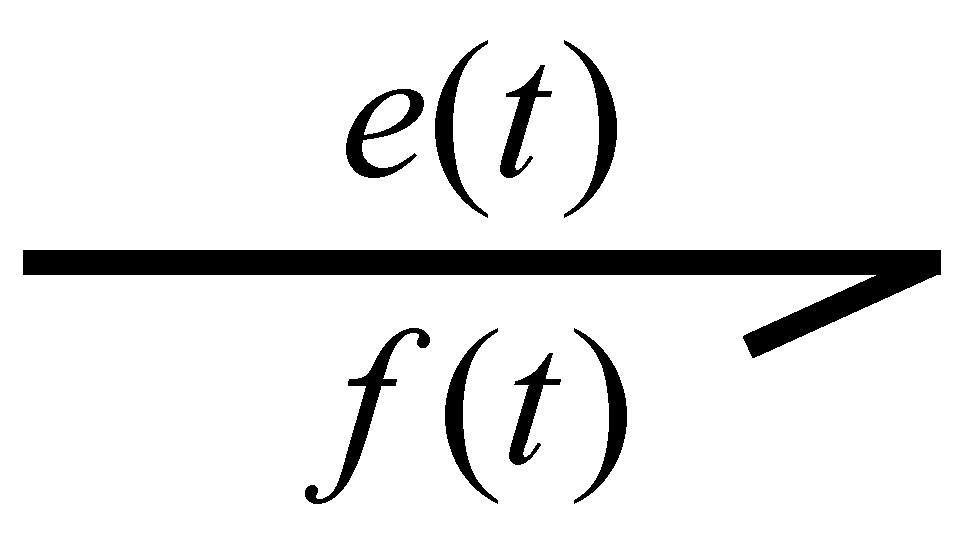
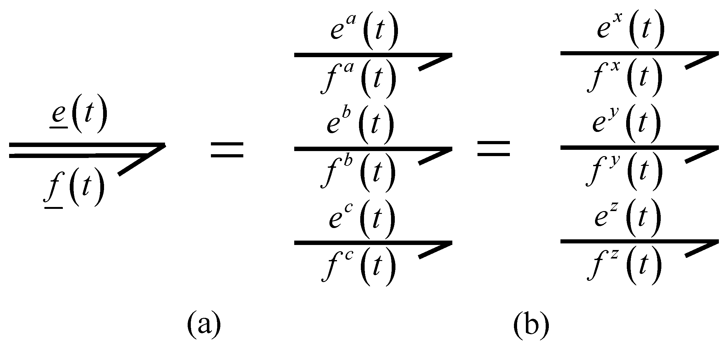
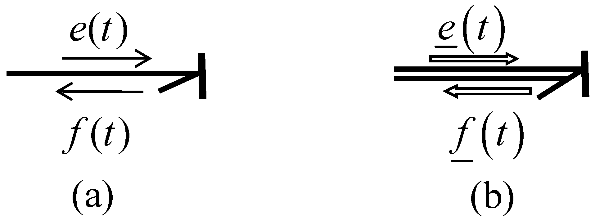
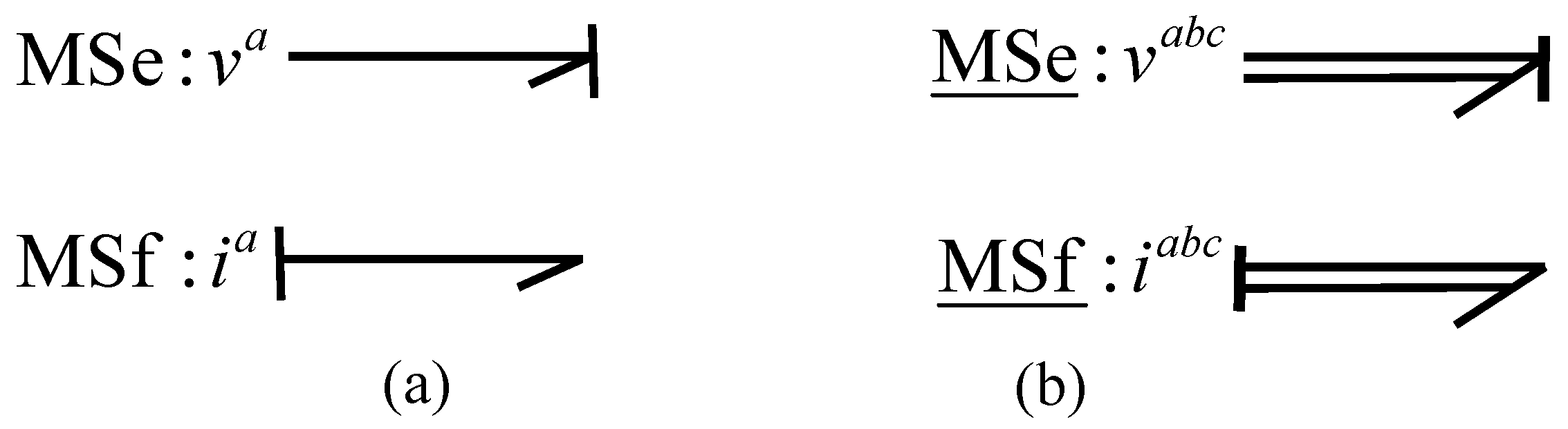
2. Modeling in Bond Graphs and Multi-Bond Graphs

When two elements, components or systems are connected, power transfer always occurs $P\left(t\right)$. Likewise, this power can be due to electrical, mechanical, hydraulic or thermal energy domains. To work in a unified frame of reference, bond graph theory uses generalized variables called effort $e\left(t\right)$ and flow $f\left(t\right)$; the main characteristics of these variables is their product, which determines the power

$$P\left(t\right)=e\left(t\right)·f\left(t\right).$$

(1)

Generalized power variables in different energy domains are indicated in Table 1.

Table 1. Power variables.

System	Effort $\mathbf{\left(}\mathit{e}\mathbf{\right(}\mathit{t}\mathbf{\left)}\mathbf{\right)}$	Flow $\mathbf{\left(}\mathit{f}\mathbf{\right(}\mathit{t}\mathbf{\left)}\mathbf{\right)}$
Electrical	Voltage $\left(v\left(t\right)\right)$	Current $\left(i\left(t\right)\right)$
Mechanical	Force $\left(F\left(t\right)\right)$ Torque $\left(\tau \left(t\right)\right)$	Velocity $\left(\nu \left(t\right)\right)$ Ang. velocity $\left(\omega \left(t\right)\right)$
Hydraulic	Pressure $\left(P\left(t\right)\right)$	Volume flow rate $\left(Q\left(t\right)\right)$
Thermodynamics	Temperature $\left(T\left(t\right)\right)$	Entropy flow $\left(S\left(t\right)\right)$

The main property of bond graph modeling is to represent power interactions graphically, as illustrated in Figure 1.

Figure 1. Power bond.

The generalization in the modeling of systems that determine power arrangements found in typical systems such as robotics and electrical in three phases has given risen to modeling with multibond graphs, for which the generalized power variables are effort and flow but in vector notation $\underline{e}\left(t\right)$ and $\underline{f}\left(t\right)$, and the power is given by

$$\underline{P}\left(t\right)={\underline{e}}^T\left(t\right)·\underline{f}\left(t\right)$$

(2)

where

$$\underline{e}\left(t\right)=\left[\begin{array}{c}{e}^a\left(t\right)\\ e^b\left(t\right)\\ e^c\left(t\right)\end{array}\right]=\left[\begin{array}{c}{e}^x\left(t\right)\\ e^y\left(t\right)\\ e^z\left(t\right)\end{array}\right]$$

(3)

and

$$\underline{f}\left(t\right)=\left[\begin{array}{c}{f}^a\left(t\right)\\ f^b\left(t\right)\\ f^c\left(t\right)\end{array}\right]=\left[\begin{array}{c}{f}^x\left(t\right)\\ f^y\left(t\right)\\ f^z\left(t\right)\end{array}\right]$$

(4)

Power interactions that are used graphically in a multibond are shown in Figure 2 along with their equivalence with bonds.

Figure 2. Multibond (a) multibond symbol, (b) multibond power equivalent individual bonds.

There are two additional variables in bond graphs to mathematically describe a system, which are the energy variables: momentum $p\left(t\right)$ and displacement $q\left(t\right)$; they are related to the power variables by

$$\begin{array}{ccc}\hfill p\left(t\right)& =& \int e\left(t\right)dt\hfill \end{array}$$

(5)

$$\begin{array}{ccc}\hfill q\left(t\right)& =& \int f\left(t\right)dt.\hfill \end{array}$$

(6)

For multibond graphs, these variables are the momentum vector and the displacement vector and are related to the power variables by

$$\begin{array}{ccc}\hfill \underline{p}\left(t\right)& =& \int \underline{e}\left(t\right)dt\hfill \end{array}$$

(7)

$$\begin{array}{ccc}\hfill \underline{q}\left(t\right)& =& \int \underline{f}\left(t\right)dt.\hfill \end{array}$$

(8)

One of the main properties of bond graph theory is the application of causality to its elements. Causality allows knowing the input and output signals for each bond or multibond. Graphically, it is applied to a vertical stroke; towards the direction of this vertical stroke, the direction of the effort is determined, and in opposition is the flow in this bond or multibond, as shown in Figure 3.

Figure 3. Causal symbols, (a) single bond graphs, (b) multibond graphs.

The basic elements to build models in bond graphs or multibond graphs are the following:

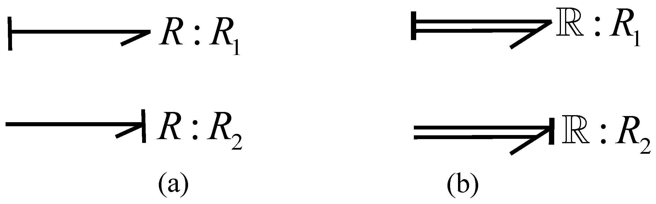
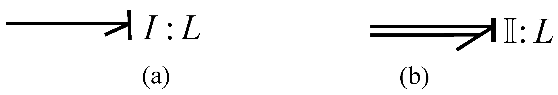
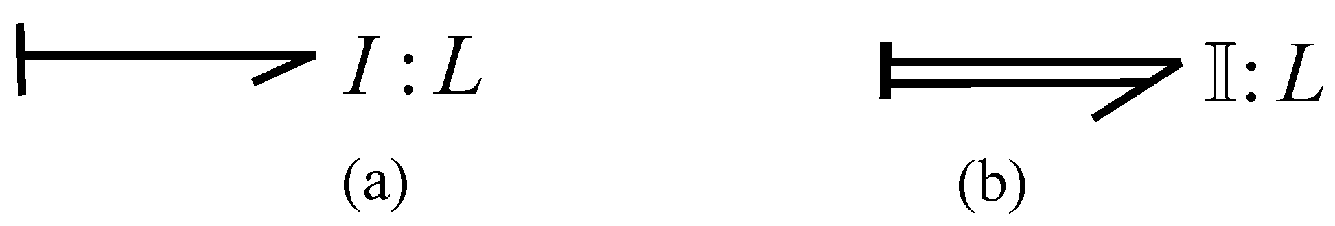
2.1. 1-Ports Active

These are the elements that supply power to the system because there are two generalized power variables, so there are two elements of this type for bonds graphs: $\left(M{S}_e,M{S}_f\right)$ effort and flow sources, respectively. In multibond graphs, $\left(\underline{M{S}_e},\underline{M{S}_f}\right)$ are the multiport effort source and multiport flow source, respectively. Figure 4 shows the representation of these sources.

Figure 4. Flow and effort sources, (a) for bond graphs, (b) multibond graphs.

2.2. 1-Ports Passive

These elements are characterized by storing or dissipating energy. The dissipative element is shown in Figure 5a, and for a multibond graph, it is shown in Figure 5b.

Figure 5. Dissipative elements for (a) single bond graphs, (b) multibond graphs.

The constitutive relationship of the element $R_1$ in a bond graph is given by

$$e\left(t\right)={\Phi }_{R_1}\left[f\left(t\right)\right]$$

(9)

In case $R_1$ is linear,

$$e\left(t\right)=R_1·f\left(t\right)$$

(10)

For $R_2$,

$$f\left(t\right)={\Phi }_{R_2}\left[e\left(t\right)\right]$$

(11)

If $R_2$ is linear,

$$f\left(t\right)=\frac{1}{R_2}e\left(t\right)$$

(12)

In a multibond graph for ${\mathbf{R}}_1$,

$$\underline{e}\left(t\right)={\Phi }_{{\mathbf{R}}_1}\left[\underline{f}\left(t\right)\right]$$

(13)

If ${\Phi }_{{\mathbf{R}}_1}$ is a linear matrix relationship of dimension 3,

$$\left[\begin{array}{c}{e}^a\left(t\right)\\ e^b\left(t\right)\\ e^c\left(t\right)\end{array}\right]=\left[\begin{array}{ccc}{R}_{11}& R_{12}& R_{13}\\ R_{21}& R_{22}& R_{23}\\ R_{31}& R_{32}& R_{33}\end{array}\right]\left[\begin{array}{c}{f}^a\left(t\right)\\ f^b\left(t\right)\\ f^c\left(t\right)\end{array}\right]$$

(14)

For the mulltiport resistor ${\mathbf{R}}_2$,

$$\underline{f}\left(t\right)={\Phi }_{{\mathbf{R}}_2}\left[\underline{e}\left(t\right)\right]$$

(15)

Its linear matrix version of dimension 3 is

$$\left[\begin{array}{c}{f}^a\left(t\right)\\ f^b\left(t\right)\\ f^c\left(t\right)\end{array}\right]=\left[\begin{array}{ccc}\frac{1}{R_{11}}& \frac{1}{R_{12}}& \frac{1}{R_{13}}\\ \frac{1}{R_{21}}& \frac{1}{R_{22}}& \frac{1}{R_{23}}\\ \frac{1}{R_{31}}& \frac{1}{R_{32}}& \frac{1}{R_{33}}\end{array}\right]\left[\begin{array}{c}{e}^a\left(t\right)\\ e^b\left(t\right)\\ e^c\left(t\right)\end{array}\right]$$

(16)

Another 1-port element is the 1-port inertia for bond graphs or the element of multiport-I for multibond graphs; these elements in an integral causality assignment are shown in Figure 6.

Figure 6. Inertia element and inertia multiport in integral causality assignment, (a) single bond graphs, (b) multibond graphs.

The constitutive relation for the storage element I of Figure 6a is defined by

$$f\left(t\right)={\Phi }_I^{-1}\left[\int e\left(t\right)dt\right]={\Phi }_I^{-1}\left[p\left(t\right)\right].$$

(17)

If this element is linear, the relationship is

$$f\left(t\right)=\frac{1}{L}\int e\left(t\right)dt=\frac{1}{L}p\left(t\right).$$

(18)

For the multiport I, the relationship between input and output is

$$\underline{f}\left(t\right)={\mathbf{\Phi }}_{\mathbf{I}}^{-1}\left[\int \underline{e}\left(t\right)dt\right]={\mathbf{\Phi }}_{\mathbf{I}}^{-1}\left[\underline{p}\left(t\right)\right]$$

(19)

For a linear multiport,

$$\underline{f}\left(t\right)={\mathbf{L}}^{-1}\int \underline{e}\left(t\right)dt={\mathbf{L}}^{-1}\underline{p}\left(t\right)$$

(20)

In expanded form,

$$\left[\begin{array}{c}{p}^a\left(t\right)\\ p^b\left(t\right)\\ p^c\left(t\right)\end{array}\right]=\left[\begin{array}{ccc}{L}_a& L_{ab}& L_{ac}\\ L_{ab}& L_b& L_{bc}\\ L_{ac}& L_{bc}& L_c\end{array}\right]\left[\begin{array}{c}{f}^a\left(t\right)\\ f^b\left(t\right)\\ f^c\left(t\right)\end{array}\right]$$

(21)

Now, if this 1-port is in derivative causality assignment, it is as shown in Figure 7.

Figure 7. Inertia element and inertia multiport in derivative causality assignment, (a) single bond graphs, (b) multibond graphs.

The constitutive relationship of element I is given by

$$e\left(t\right)={\displaystyle \frac{d{\Phi }_I\left[f\left(t\right)\right]}{dt}}$$

(22)

If it is a lineal element,

$$e\left(t\right)=L{\displaystyle \frac{d\left[f\left(t\right)\right]}{dt}}$$

(23)

For multiport $\mathbb{I}$, its relationship is

$$\underline{e}\left(t\right)={\displaystyle \frac{d{\mathbf{\Phi }}_{\mathbf{I}}\left[\underline{f}\left(t\right)\right]}{dt}}$$

(24)

If it is a linear element, we have

$$\left[\begin{array}{c}{e}^a\left(t\right)\\ e^b\left(t\right)\\ e^c\left(t\right)\end{array}\right]=\left[\begin{array}{ccc}{L}_a& L_{ab}& L_{ac}\\ L_{ab}& L_b& L_{bc}\\ L_{ac}& L_{bc}& L_c\end{array}\right]\left[\begin{array}{c}\frac{d{f}^a\left(t\right)}{dt}\\ \frac{d{f}^b\left(t\right)}{dt}\\ \frac{d{f}^c\left(t\right)}{dt}\end{array}\right]$$

(25)

The other storage element is the capacitance in an integral causality assignment, as illustrated in Figure 8.

Figure 8. Capacitor element and capacitor multiport in integral causality assignment, (a) single bond graphs, (b) multibond graphs.

The constitutive relation for element C is defined by

$$e\left(t\right)={\Phi }_C^{-1}\left[\int f\left(t\right)dt\right]={\Phi }_C^{-1}\left[q\left(t\right)\right]$$

(26)

If this element is linear,

$$e\left(t\right)=\frac{1}{C}\int f\left(t\right)dt=\frac{1}{C}q\left(t\right)$$

(27)

The constitutive relation for multiport $\mathbb{C}$ is expressed by

$$\underline{e}\left(t\right)={\mathbf{\Phi }}_{\mathbf{C}}^{-1}\left[\int \underline{f}\left(t\right)dt\right]={\mathbf{\Phi }}_{\mathbf{C}}^{-1}\left[\underline{q}\left(t\right)\right]$$

(28)

Considering a linear multiport element,

$$\underline{e}\left(t\right)={\mathbf{C}}^{-1}\int \underline{f}\left(t\right)dt={\mathbf{C}}^{-1}\underline{q}\left(t\right)$$

(29)

In expanded form,

$$\left[\begin{array}{c}{q}^a\left(t\right)\\ q^b\left(t\right)\\ q^c\left(t\right)\end{array}\right]=\left[\begin{array}{ccc}{C}_a& C_{ab}& C_{ac}\\ C_{ab}& C_b& C_{bc}\\ C_{ac}& C_{bc}& C_c\end{array}\right]\left[\begin{array}{c}{e}^a\left(t\right)\\ e^b\left(t\right)\\ e^c\left(t\right)\end{array}\right]$$

(30)

This element in a derivative causality assignment is shown in Figure 9.

Figure 9. Capacitor element and capacitor multiport in derivative causality assignment, (a) single bond graphs, (b) multibond graphs.

For element C, its constitutive relationship is

$$f\left(t\right)={\displaystyle \frac{d{\Phi }_C\left[e\left(t\right)\right]}{dt}}$$

(31)

With a linear relationship,

$$f\left(t\right)=C{\displaystyle \frac{d\left[e\left(t\right)\right]}{dt}}$$

(32)

For multiport $\mathbb{C}$, the constitutive relation is

$$\underline{f}\left(t\right)={\displaystyle \frac{d{\mathbf{\Phi }}_{\mathbf{C}}\left[\underline{e}\left(t\right)\right]}{dt}}$$

(33)

For the linear case,

$$\left[\begin{array}{c}{f}^a\left(t\right)\\ f^b\left(t\right)\\ f^c\left(t\right)\end{array}\right]=\left[\begin{array}{ccc}{C}_a& C_{ab}& C_{ac}\\ C_{ab}& C_b& C_{bc}\\ C_{ac}& C_{bc}& C_c\end{array}\right]\left[\begin{array}{c}\frac{d{e}^a\left(t\right)}{dt}\\ \frac{d{e}^b\left(t\right)}{dt}\\ \frac{d{e}^c\left(t\right)}{dt}\end{array}\right]$$

(34)

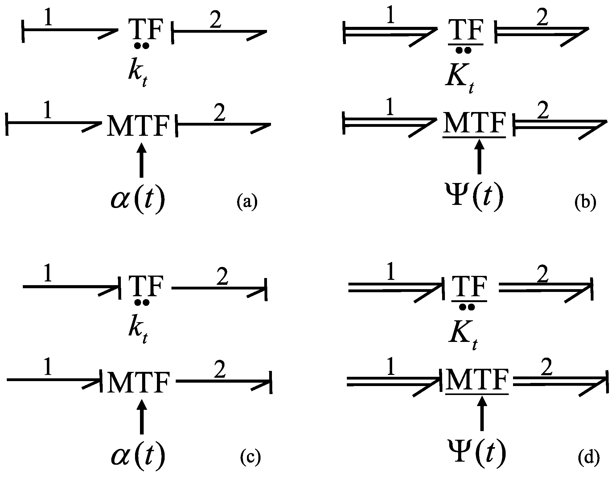
2.3. 2-Ports

Important elements in the transfer of power between various sections of a system are modeled in bond graph by transformers and gyrators modulated by a constant magnitude or by a signal, as shown in Figure 10.

Figure 10. Transformer, (a) single bond graphs, (b) multiport bond graphs, (c) sigle bond with reversed causality and (d) multiport bond graphs with reversed causality and multiport transformer.

Depending on the causality, the constitutive relationship between the ports of a transformer may be different as presented in [23]. Thus, for Figure 10a, the relations are given by

$$\left[\begin{array}{c}{e}_1\\ f_1\end{array}\right]=\left[\begin{array}{cc}{k}_t& 0\\ 0& {\displaystyle \frac{1}{k_t}}\end{array}\right]\left[\begin{array}{c}{e}_2\\ f_2\end{array}\right]$$

(35)

where $k_t$ is the constant modulus for a transformer $\left(TF\right)$, and for a modulated transformer $\left(MTF\right)$, $k_t=\alpha \left(t\right)$.

For the transformer with a causality illustrated in Figure 10c, the port relations are

$$\left[\begin{array}{c}{e}_2\\ f_2\end{array}\right]=\left[\begin{array}{cc}{k}_t& 0\\ 0& {\displaystyle \frac{1}{k_t}}\end{array}\right]\left[\begin{array}{c}{e}_1\\ f_1\end{array}\right]$$

(36)

The multiport transformer has constitutive relations defined by

$$\left[\begin{array}{c}\underline{e_1}\\ \underline{f_1}\end{array}\right]=\left[\begin{array}{cc}{K}_t& 0\\ 0& K_t^{-1}\end{array}\right]\left[\begin{array}{c}\underline{e_2}\\ \underline{f_2}\end{array}\right]$$

(37)

where $K_t$ is the constant modulus matrix for a multiport transformer $\left(\underline{TF}\right)$, and for a multiport modulated transformer $\left(\underline{MTF}\right)$, $M_t=\Psi \left(t\right)$.

For a multiport transformer with the causality shown in Figure 10d, the multibond relations are

$$\left[\begin{array}{c}\underline{e_1}\\ \underline{f_1}\end{array}\right]=\left[\begin{array}{cc}{K}_t^{-1}& 0\\ 0& K_t\end{array}\right]\left[\begin{array}{c}\underline{e_2}\\ \underline{f_2}\end{array}\right]$$

(38)

Another important element of port-2 represents the gyrators illustrated in Figure 11.

Figure 11. Gyrator and multiport gyrator, (a) single bond graphs, (b) multiport bond graphs, (c) sigle bond with reversed causality and (d) multiport bond graphs with reversed causality.

The constitutive relation for the gyrator $\left(GY\right)$ of Figure 11 is expressed by

$$\left[\begin{array}{c}{e}_1\\ f_1\end{array}\right]=\left[\begin{array}{cc}0& k_g\\ {\displaystyle \frac{1}{k_g}}& 0\end{array}\right]\left[\begin{array}{c}{e}_2\\ f_2\end{array}\right]$$

(39)

where $k_g$ is the constant modulus for a gyrator $\left(GY\right)$, and for a modulated gyrator $\left(MGY\right)$, $k_g=\beta \left(t\right)$.

If the gyrator has a causality like the one shown in Figure 11c, the constitutive relation is

$$\left[\begin{array}{c}{e}_1\\ f_1\end{array}\right]=\left[\begin{array}{cc}0& {\displaystyle \frac{1}{k_g}}\\ k_g& 0\end{array}\right]\left[\begin{array}{c}{e}_2\\ f_2\end{array}\right]$$

(40)

In case it is a modulated gyrator $\left(MGY\right)$, $k_g=\beta \left(t\right)$.

The multiport gyrator of Figure 11b has the constitutive relation given by

$$\left[\begin{array}{c}{e}_1\\ f_1\end{array}\right]=\left[\begin{array}{cc}0& K_g\\ K_g^{-1}& 0\end{array}\right]\left[\begin{array}{c}{e}_2\\ f_2\end{array}\right]$$

(41)

where $K_g$ is the modulo constant matrix for a multiport gyrator $\left(\underline{GY}\right)$, and for a modulated multiport gyrator $\left(\underline{MGY}\right)$, $K_g=\Lambda \left(t\right)$.

In case the gyrator is in a causality like the one shown in Figure 11d, the relationship is defined by

$$\left[\begin{array}{c}{e}_1\\ f_1\end{array}\right]=\left[\begin{array}{cc}0& K_g\\ K_g^{-1}& 0\end{array}\right]\left[\begin{array}{c}{e}_2\\ f_2\end{array}\right]$$

(42)

In case it is a modulated gyrator $\left(MGY\right)$, $k_g=\beta \left(t\right)$.

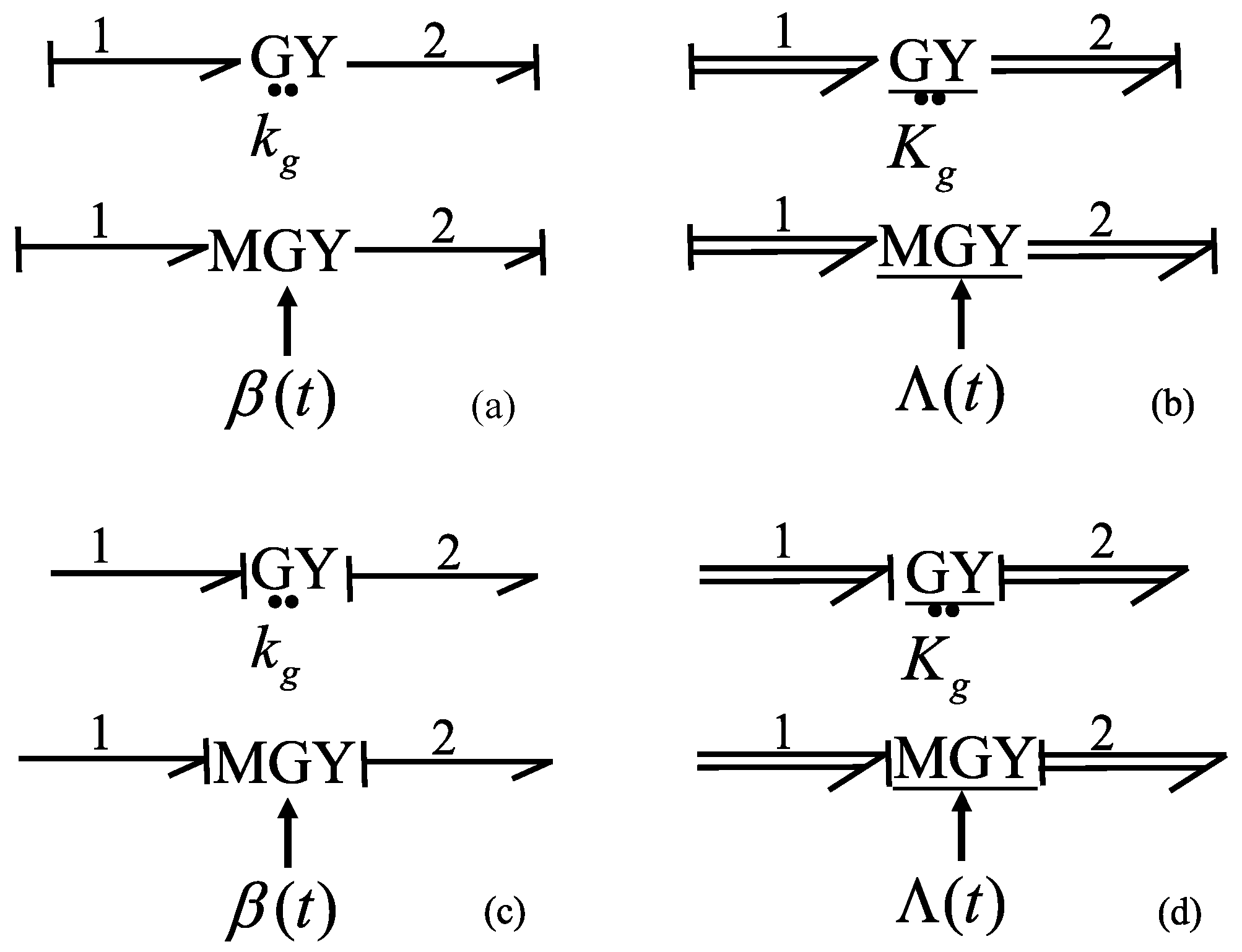
2.4. 3-Ports

3-ports represent the serial (1-junction) and parallel (0-junction) connections in the different physical systems. These junctions are conservative power elements, which are shown in Figure 12.

Figure 12. (a) Single-element junctions and (b) mutltiport junctions.

The junctions are the elements that allow the connection of the elements and form the bond graph models for which the constitutive relations for 1-junction are given by

$$e_1=e_2+e_3;f_1=f_2=f_3$$

(43)

and for 0-junction, they are

$$e_1=e_2=e_3;f_1=f_2+f_3$$

(44)

The effort and flow relationships of multibonds applied to junctions 1 and 0 are similar to the previous ones considering that they have vectors: for 1-junction

$$\underline{e_1}=\underline{e_2}+\underline{e_3};\underline{f_1}=\underline{f_2}=\underline{f_3}$$

(45)

and for the other junction

$$\underline{e_1}=\underline{e_2}=\underline{e_3};\underline{f_1}=\underline{f_2}+\underline{f_3}$$

(46)

A junction structure of a system modeled by a multibond graph connected to a bond graph is proposed in the next section.

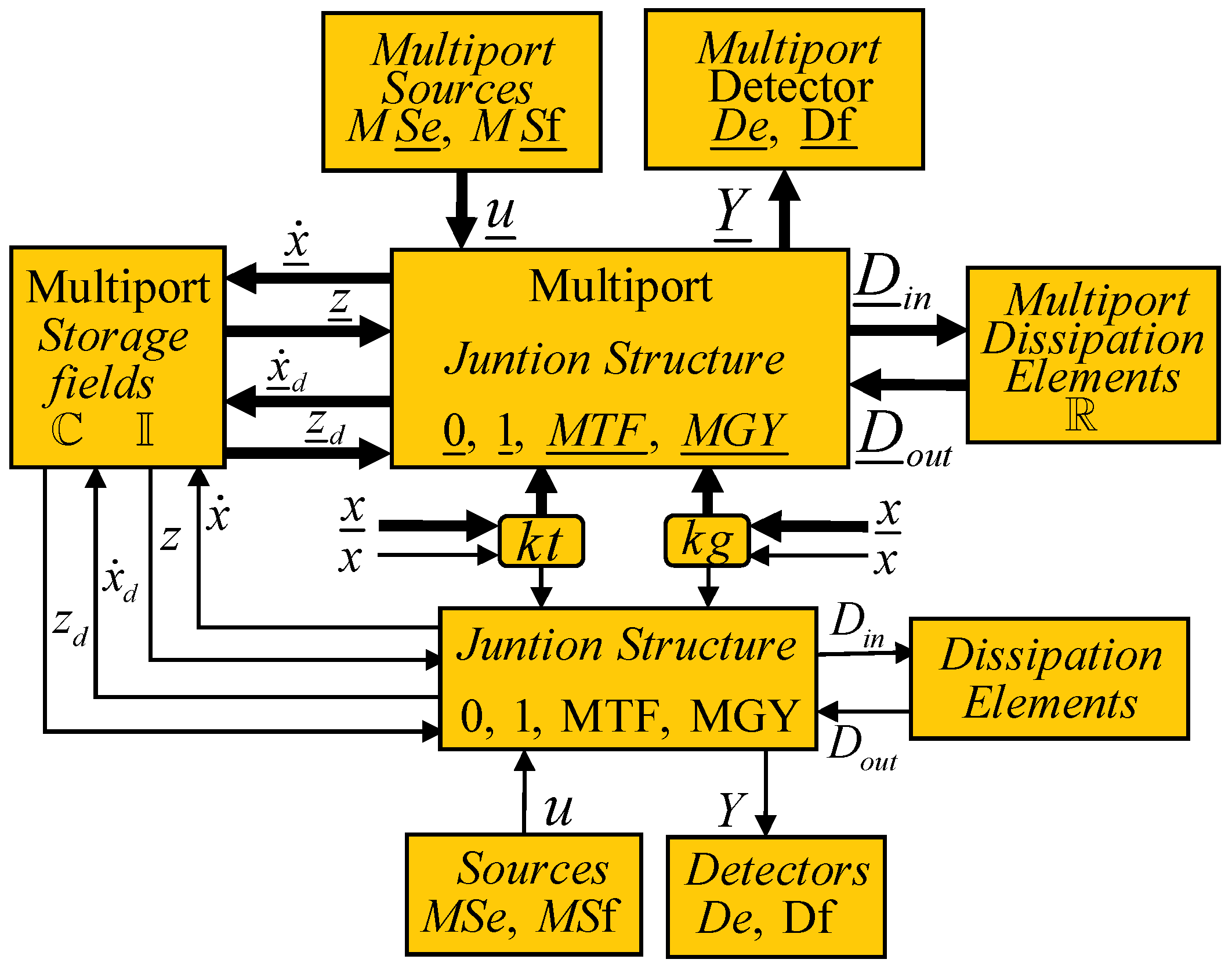
3. A Mathematical Model of a System Composed of MultiBond Graphs and Bond Graphs

Some systems that are defined on three axes and modeled by bond graphs can lead to very extensive and complicated models. These types of systems modeled by multibond graphs can determine a compact and organized model.

However, many systems with three-axis actuators and controllers are individual for each axis. Thus, modeling these systems in multibond graphs can result in multibond graphs with multibonds with non-complete signals: that is, multibonds that, mathematically represented, determine vectors with one non-zero element and the rest with zeros. Due to this, the utility of multibond graphs is not used for these signals.

Therefore, it is possible to model three-axis systems with multibond graphs in which one axis can contain the actuator and control subsystems modeled by bond graphs. In order to have analysis tools for these systems with three coordinates linked to subsystems of one coordinate, the determination of the mathematical model of the same is required. The proposed junction structure for ($MBG$-$BG$) is shown in Figure 13.

Figure 13. Junction structure for ($MBG$-$BG$).

The block diagram information representing a multibond graph and bond graph determines the following elements and key vectors:

• Bond graph section:

  –

  Elements of energy supply sources denoted by $\left(M{S}_e,M{S}_f\right)$ with variables $u\left(t\right)\in {\Re }^p.$

  –

  Energy storage elements denoted by $\left(C,I\right)$:

  *

  In integral causality assignment with state variables $x\left(t\right)\in {\Re }^n$ and co-energy vector $z\left(t\right)\in {\Re }^n$ determining linearly independent state variables.

  *

  In derivative causality assignment with state variables $x_d\left(t\right)\in {\Re }^m$ and co-energy vector $z_d\left(t\right)\in {\Re }^m$ determining linearly dependent state variables.

  –

  Detection elements for system outputs denoted by $\left(D_e,D_f\right)$ with variables $y\left(t\right)\in {\Re }^q$.

  –

  Energy dissipation elements denoted by $\left(R\right)$ with variables $D_{in}\left(t\right)\in {\Re }^r$ and $D_{out}\left(t\right)\in {\Re }^r$.

  –

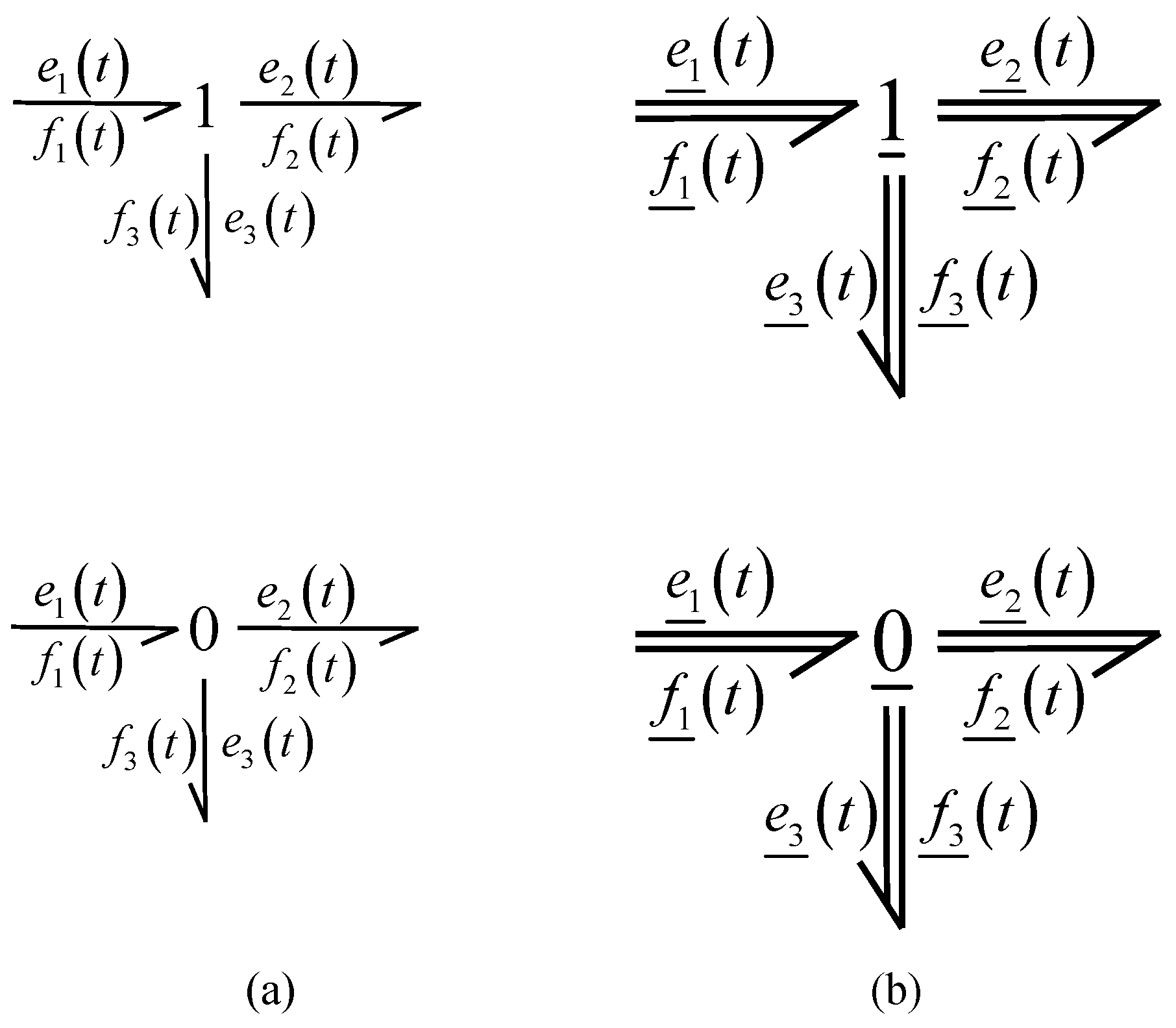
  The different elements of a system $\left(M{S}_e,M{S}_f\right)$, $\left(C,I\right)$, $\left(D_e,D_f\right)$ and $\left(R\right)$ are connected by the 0 and 1 junctions or by transformers $\left(MTF\right)$ and gyrators $\left(MGY\right)$ modulated by variables or constants.

• Multibond graph section:

  –

  Source multiport elements denoted by $\left(\underline{MSe},\underline{MSf}\right)$ with multiport input variables $\underline{u}\left(t\right)\in {\Re }^{\underline{p}}.$

  –

  Storage multiport fields denoted by $\left(\mathbb{C},II\right)$:

  *

  In integral causality assignment with multiport state variables $\underline{x}\left(t\right)\in {\Re }^{\underline{n}}$ and multiport co-energy vector $\underline{z}\left(t\right)\in {\Re }^{\underline{n}}$ that determine linearly independent multiport state variables.

  *

  In derivative causality assignment with multiport state variables $\underline{x_d}\left(t\right)\in {\Re }^{\underline{m}}$ and multiport co-energy vector $\underline{z_d}\left(t\right)\in {\Re }^{\underline{m}}$ that determine linearly dependent multiport state variables.

  *

  These fields can be used to connect the multibond graph and bond graph sections according to the system characteristics.

  –

  Multiport detection elements denoted by $\left(\underline{De},\underline{D_f}\right)$ with multiport outputs $\underline{y}\left(t\right)\in {\Re }^{\underline{q}}$.

  –

  Multiport energy dissipation denoted by $\left(\mathbb{R}\right)$ with multiport variables $\underline{D_{in}}\in {\Re }^{\underline{r}}$ and $\underline{D_{out}}\in {\Re }^{\underline{r}}$.

  –

  Multiport junctions $\left(\underline{0},\underline{1}\right)$, modulated multiport transformers $\left(\underline{MTF}\right)$ and modulated multiport gyrators $\left(\underline{MGY}\right)$ are used to connect the different multiport elements $\left(\underline{MSe},\underline{MSf}\right)$, $\left(\mathbb{C},II\right)$, $\left(\underline{De},\underline{D_f}\right)$ and $\left(\mathbb{R}\right)$. In addition, these transformers or gyrators can be used to connect this section of the multibond graph with the section of the bond graph.

According to the proposed junction structure of Figure 13, the connection between multibond graphs and bond graphs is through multiport transformers and gyrators or through multiport energy storage fields. Thus, for the multiport field of $\left(\mathbb{C},II\right)$ in an integral causality assignment, the constitutive relation is defined by

$$\left[\begin{array}{c}\underline{z}\left(t\right)\\ z\left(t\right)\end{array}\right]=\left[\begin{array}{cc}\mathbf{F}& {\mathbf{F}}_m\\ F_m^T& F\end{array}\right]\left[\begin{array}{c}\underline{x}\left(t\right)\\ x\left(t\right)\end{array}\right]$$

(47)

For multiport elements $\left(\mathbb{C},II\right)$ in derivative causality and for resistive multiport $\left(\mathbb{R}\right)$, they are expressed by

$$\begin{array}{ccc}\hfill \underline{z_d}\left(t\right)& =& {\mathbf{F}}_d\underline{x_d}\left(t\right)\hfill \end{array}$$

(48)

$$\begin{array}{ccc}\hfill \underline{D_{out}}\left(t\right)& =& \mathbf{L}\underline{D_{in}}\left(t\right)\hfill \end{array}$$

(49)

For the elements $\left(C,I\right)$ in derivative causality and for dissipative elements $\left(R\right)$, they are given by

$$\begin{array}{ccc}\hfill z_d\left(t\right)& =& F_d{x}_d\left(t\right)\hfill \end{array}$$

(50)

$$\begin{array}{ccc}\hfill D_{out}\left(t\right)& =& L{D}_{in}\left(t\right)\hfill \end{array}$$

(51)

The scheme in Figure 13 for modeling $\left(MBG-BGI\right)$ systems determines a class of nonlinear systems representative of products of state variables for which the characteristics are defined in the following lemma.

Lemma 1.

Consider a system modeled by multibond graphs and bond graphs $\left(MBG-BGI\right)$ with a predefined integral causality assignment according to Figure 13. The connection between them is described by transformers and/or gyrators and/or storage fields for which the combined multiport junction structure is defined by

$$\left[\begin{array}{c}\underline{\stackrel{•}{x}}\left(t\right)\\ \stackrel{•}{x}\left(t\right)\\ \underline{D_{in}}\left(t\right)\\ D_{in}\left(t\right)\\ \underline{y}\left(t\right)\\ y\left(t\right)\\ \underline{z_d}\left(t\right)\\ z_d\left(t\right)\end{array}\right]=\left[\begin{array}{cccccccc}{\mathbf{S}}_{11}^{11}\left(\underline{x}\right)& {\mathbf{S}}_{11}^{12}\left(\underline{x}\right)& {\mathbf{S}}_{12}^{11}\left(\underline{x}\right)& {\mathbf{S}}_{12}^{12}\left(\underline{x}\right)& {\mathbf{S}}_{13}^{11}\left(\underline{x}\right)& {\mathbf{S}}_{13}^{12}\left(\underline{x}\right)& {\mathbf{S}}_{14}^{11}\left(\underline{x}\right)& 0\\ S_{11}^{21}\left(x\right)& S_{11}^{22}\left(x\right)& S_{12}^{21}\left(x\right)& S_{12}^{22}\left(x\right)& S_{13}^{21}\left(x\right)& S_{13}^{22}\left(x\right)& 0& S_{14}^{22}\left(x\right)\\ {\mathbf{S}}_{21}^{11}\left(\underline{x}\right)& {\mathbf{S}}_{21}^{12}\left(\underline{x}\right)& {\mathbf{S}}_{22}^{11}\left(\underline{x}\right)& 0& {\mathbf{S}}_{23}^{11}\left(\underline{x}\right)& {\mathbf{S}}_{23}^{12}\left(\underline{x}\right)& 0& 0\\ S_{21}^{21}\left(x\right)& S_{21}^{22}\left(x\right)& 0& S_{22}^{22}\left(x\right)& S_{23}^{21}\left(x\right)& S_{23}^{22}\left(x\right)& 0& 0\\ {\mathbf{S}}_{31}^{11}\left(\underline{x}\right)& {\mathbf{S}}_{31}^{12}\left(\underline{x}\right)& {\mathbf{S}}_{32}^{11}\left(\underline{x}\right)& {\mathbf{S}}_{32}^{12}\left(\underline{x}\right)& {\mathbf{S}}_{33}^{11}\left(\underline{x}\right)& {\mathbf{S}}_{33}^{12}\left(\underline{x}\right)& 0& 0\\ S_{31}^{21}\left(x\right)& S_{31}^{22}\left(x\right)& S_{32}^{21}\left(x\right)& S_{32}^{22}\left(x\right)& S_{33}^{21}\left(x\right)& S_{33}^{22}\left(x\right)& 0& 0\\ {\mathbf{S}}_{41}^{11}\left(\underline{x}\right)& 0& 0& 0& 0& 0& 0& 0\\ 0& S_{41}^{22}\left(x\right)& 0& 0& 0& 0& 0& 0\end{array}\right]\left[\begin{array}{c}\underline{z}\left(t\right)\\ z\left(t\right)\\ \underline{D_{out}}\left(t\right)\\ D_{out}\left(t\right)\\ \underline{u}\left(t\right)\\ u\left(t\right)\\ \underline{{\stackrel{•}{x}}_d}\left(t\right)\\ {\stackrel{•}{x}}_d\left(t\right)\end{array}\right]$$

(52)

Then a nonlinear state-space representation is given by

$$\mathbf{E}\left(\underline{x}\right)\left[\begin{array}{c}\underline{\stackrel{•}{x}}\left(t\right)\\ \stackrel{•}{x}\left(t\right)\end{array}\right]=\mathbf{A}\left(\underline{x}\right)\left[\begin{array}{c}\underline{x}\left(t\right)\\ x\left(t\right)\end{array}\right]+\mathbf{B}\left(\underline{x}\right)\left[\begin{array}{c}\underline{u}\left(t\right)\\ u\left(t\right)\end{array}\right]$$

(53)

where

$$\mathbf{E}\left(\underline{x}\right)=\left[\begin{array}{cc}{\mathbf{E}}_{11}\left(\underline{x}\right)& {\mathbf{E}}_{12}\left(\underline{x}\right)\\ E_{21}\left(x\right)& E_{22}\left(x\right)\end{array}\right]=\left[\begin{array}{cc}I-{\mathbf{S}}_{14}^{11}\left(\underline{x}\right){\mathbf{F}}_d{\mathbf{S}}_{41}^{11}\left(x\right)\mathbf{F}& -{\mathbf{S}}_{14}^{11}\left(\underline{x}\right){\mathbf{F}}_d^{-1}{\mathbf{S}}_{41}^{11}\left(x\right){\mathbf{F}}_m\\ -S_{14}^{22}\left(x\right)F_d^{-1}{S}_{41}^{22}\left(x\right)F_m^T& I-S_{14}^{22}\left(x\right)F_d^{-1}{S}_{41}^{22}\left(x\right)F\end{array}\right]$$

(54)

$$\mathbf{A}\left(\underline{x}\right)=\left[\begin{array}{cc}{\mathbf{A}}_{11}\left(\underline{x}\right)& {\mathbf{A}}_{12}\left(\underline{x}\right)\\ A_{21}\left(x\right)& A_{22}\left(x\right)\end{array}\right]=\left[\begin{array}{cc}{\mathbf{A}}_{11}^{\prime }\left(\underline{x}\right)\mathbf{F}+{\mathbf{A}}_{12}^{\prime }\left(\underline{x}\right)F_m^T& {\mathbf{A}}_{11}^{\prime }\left(\underline{x}\right){\mathbf{F}}_m+{\mathbf{A}}_{12}^{\prime }\left(\underline{x}\right)\mathbf{F}\\ A_{21}^{\prime }\left(x\right)\mathbf{F}+A_{22}^{\prime }\left(x\right)F_m^T& A_{21}^{\prime }\left(x\right){\mathbf{F}}_m+A_{22}^{\prime }\left(x\right)F\end{array}\right]$$

(55)

with

$$\begin{array}{ccc}\hfill {\mathbf{A}}_{11}^{\prime }\left(\underline{x}\right)& =& {\mathbf{S}}_{11}^{11}\left(\underline{x}\right)+{\mathbf{S}}_{12}^{11}\left(\underline{x}\right)\mathbf{M}\left(\underline{x}\right){\mathbf{S}}_{21}^{11}\left(\underline{x}\right)+{\mathbf{S}}_{12}^{12}\left(\underline{x}\right)M\left(x\right)S_{21}^{21}\left(x\right)\hfill \end{array}$$

(56)

$$\begin{array}{ccc}\hfill {\mathbf{A}}_{12}^{\prime }\left(\underline{x}\right)& =& {\mathbf{S}}_{11}^{12}\left(\underline{x}\right)+{\mathbf{S}}_{12}^{11}\left(\underline{x}\right)\mathbf{M}\left(\underline{x}\right){\mathbf{S}}_{21}^{12}\left(\underline{x}\right)+{\mathbf{S}}_{12}^{12}\left(\underline{x}\right)M\left(x\right)S_{21}^{22}\left(x\right)\hfill \end{array}$$

(57)

$$\begin{array}{ccc}\hfill A_{21}^{\prime }\left(\underline{x}\right)& =& S_{11}^{21}\left(x\right)+S_{12}^{21}\left(x\right)\mathbf{M}\left(x\right){\mathbf{S}}_{21}^{11}\left(\underline{x}\right)+S_{12}^{22}\left(x\right)M\left(x\right)S_{21}^{21}\left(x\right)\hfill \end{array}$$

(58)

$$\begin{array}{ccc}\hfill A_{22}^{\prime }\left(x\right)& =& S_{11}^{22}\left(x\right)+S_{12}^{21}\left(x\right)\mathbf{M}\left(x\right){\mathbf{S}}_{21}^{12}\left(\underline{x}\right)+S_{12}^{22}\left(x\right)M\left(x\right)S_{21}^{22}\left(x\right)\hfill \end{array}$$

(59)

$$\mathbf{B}\left(\underline{x}\right)=\left[\begin{array}{cc}{\mathbf{B}}_{11}\left(\underline{x}\right)& {\mathbf{B}}_{12}\left(\underline{x}\right)\\ B_{21}\left(x\right)& B_{22}\left(x\right)\end{array}\right]$$

(60)

$$\begin{array}{ccc}\hfill {\mathbf{B}}_{11}\left(\underline{x}\right)& =& {\mathbf{S}}_{13}^{11}\left(\underline{x}\right)+{\mathbf{S}}_{12}^{11}\left(\underline{x}\right)\mathbf{M}\left(\underline{x}\right){\mathbf{S}}_{23}^{11}\left(x\right)+{\mathbf{S}}_{12}^{12}\left(\underline{x}\right)M\left(x\right)S_{23}^{21}\left(x\right)\hfill \end{array}$$

(61)

$$\begin{array}{ccc}\hfill {\mathbf{B}}_{12}\left(\underline{x}\right)& =& {\mathbf{S}}_{13}^{12}\left(\underline{x}\right)+{\mathbf{S}}_{12}^{11}\left(\underline{x}\right)\mathbf{M}\left(\underline{x}\right){\mathbf{S}}_{23}^{12}\left(x\right)+{\mathbf{S}}_{12}^{12}\left(\underline{x}\right)M\left(x\right)S_{23}^{22}\left(x\right)\hfill \end{array}$$

(62)

$$\begin{array}{ccc}\hfill B_{21}\left(x\right)& =& S_{13}^{21}\left(x\right)+S_{12}^{21}\left(x\right)M\left(x\right){\mathbf{S}}_{23}^{11}\left(x\right)+S_{12}^{22}\left(x\right)M\left(x\right)S_{23}^{21}\left(x\right)\hfill \end{array}$$

(63)

$$\begin{array}{ccc}\hfill B_{22}\left(x\right)& =& S_{13}^{22}\left(x\right)+S_{12}^{21}\left(x\right)M\left(x\right){\mathbf{S}}_{23}^{12}\left(x\right)+S_{12}^{22}\left(x\right)M\left(x\right)S_{23}^{22}\left(x\right)\hfill \end{array}$$

(64)

being

$$\begin{array}{ccc}\hfill \mathbf{M}\left(\underline{x}\right)& =& \mathbf{L}{\left[I-{\mathbf{S}}_{22}^{11}\left(\underline{x}\right)\mathbf{L}\right]}^{-1}\hfill \end{array}$$

(65)

$$\begin{array}{ccc}\hfill M\left(x\right)& =& L{\left[I-S_{22}^{22}\left(x\right)L\right]}^{-1}\hfill \end{array}$$

(66)

with system outputs

$$\left[\begin{array}{c}\underline{y}\left(t\right)\\ y\left(t\right)\end{array}\right]=\mathbf{C}\left(\underline{x}\right)\left[\begin{array}{c}\underline{x}\left(t\right)\\ x\left(t\right)\end{array}\right]+\mathbf{D}\left(\underline{x}\right)\left[\begin{array}{c}\underline{u}\left(t\right)\\ u\left(t\right)\end{array}\right]$$

(67)

where

$$\mathbf{C}\left(\underline{x}\right)=\left[\begin{array}{cc}{\mathbf{C}}_{11}\left(\underline{x}\right)& {\mathbf{C}}_{12}\left(\underline{x}\right)\\ C_{21}\left(x\right)& C_{22}\left(x\right)\end{array}\right]=\left[\begin{array}{cc}{\mathbf{C}}_{11}^{\prime }\left(\underline{x}\right)\mathbf{F}+{\mathbf{C}}_{12}^{\prime }\left(\underline{x}\right)F_m^T& {\mathbf{C}}_{11}^{\prime }\left(\underline{x}\right){\mathbf{F}}_m+{\mathbf{C}}_{12}^{\prime }\left(\underline{x}\right)\mathbf{F}\\ C_{21}^{\prime }\left(x\right)\mathbf{F}+C_{22}^{\prime }\left(x\right)F_m^T& C_{21}^{\prime }\left(x\right){\mathbf{F}}_m+C_{22}^{\prime }\left(x\right)F\end{array}\right]$$

(68)

$$\begin{array}{ccc}\hfill {\mathbf{C}}_{11}^{\prime }\left(\underline{x}\right)& =& {\mathbf{S}}_{31}^{11}\left(\underline{x}\right)+{\mathbf{S}}_{32}^{11}\left(\underline{x}\right)\mathbf{M}\left(\underline{x}\right){\mathbf{S}}_{21}^{11}\left(\underline{x}\right)+{\mathbf{S}}_{32}^{12}\left(\underline{x}\right)M\left(x\right)S_{21}^{21}\left(x\right)\hfill \end{array}$$

(69)

$$\begin{array}{ccc}\hfill {\mathbf{C}}_{12}^{\prime }\left(\underline{x}\right)& =& {\mathbf{S}}_{31}^{12}\left(\underline{x}\right)+{\mathbf{S}}_{32}^{11}\left(\underline{x}\right)\mathbf{M}\left(\underline{x}\right){\mathbf{S}}_{21}^{12}\left(\underline{x}\right)+{\mathbf{S}}_{32}^{12}\left(\underline{x}\right)M\left(x\right)S_{21}^{22}\left(x\right)\hfill \end{array}$$

(70)

$$\begin{array}{ccc}\hfill C_{21}^{\prime }\left(\underline{x}\right)& =& S_{31}^{21}\left(\underline{x}\right)+S_{32}^{21}\left(x\right)\mathbf{M}\left(\underline{x}\right){\mathbf{S}}_{21}^{11}\left(\underline{x}\right)+S_{32}^{22}\left(x\right)M\left(x\right)S_{21}^{21}\left(x\right)\hfill \end{array}$$

(71)

$$\begin{array}{ccc}\hfill C_{22}^{\prime }\left(\underline{x}\right)& =& S_{31}^{22}\left(\underline{x}\right)+S_{32}^{21}\left(x\right)\mathbf{M}\left(\underline{x}\right){\mathbf{S}}_{21}^{12}\left(\underline{x}\right)+S_{32}^{22}\left(x\right)M\left(x\right)S_{21}^{22}\left(x\right)\hfill \end{array}$$

(72)

$$\mathbf{D}\left(\underline{x}\right)=\left[\begin{array}{cc}{\mathbf{D}}_{11}\left(\underline{x}\right)& {\mathbf{D}}_{12}\left(\underline{x}\right)\\ D_{21}\left(x\right)& D_{22}\left(x\right)\end{array}\right]$$

(73)

$$\begin{array}{ccc}\hfill {\mathbf{D}}_{11}\left(\underline{x}\right)& =& {\mathbf{S}}_{33}^{11}\left(\underline{x}\right)+{\mathbf{S}}_{32}^{11}\left(\underline{x}\right)\mathbf{M}\left(\underline{x}\right){\mathbf{S}}_{23}^{11}\left(x\right)+{\mathbf{S}}_{32}^{12}\left(\underline{x}\right)M\left(x\right)S_{23}^{21}\left(x\right)\hfill \end{array}$$

(74)

$$\begin{array}{ccc}\hfill {\mathbf{D}}_{12}\left(\underline{x}\right)& =& {\mathbf{S}}_{33}^{12}\left(\underline{x}\right)+{\mathbf{S}}_{32}^{11}\left(\underline{x}\right)\mathbf{M}\left(\underline{x}\right){\mathbf{S}}_{23}^{12}\left(x\right)+{\mathbf{S}}_{32}^{12}\left(\underline{x}\right)M\left(x\right)S_{23}^{22}\left(x\right)\hfill \end{array}$$

(75)

$$\begin{array}{ccc}\hfill D_{21}\left(x\right)& =& S_{33}^{21}\left(x\right)+S_{32}^{21}\left(x\right)\mathbf{M}\left(x\right){\mathbf{S}}_{23}^{11}\left(x\right)+S_{32}^{22}\left(x\right)M\left(x\right)S_{23}^{21}\left(x\right)\hfill \end{array}$$

(76)

$$\begin{array}{ccc}\hfill D_{21}\left(x\right)& =& S_{33}^{21}\left(x\right)+S_{32}^{21}\left(x\right)\mathbf{M}\left(x\right){\mathbf{S}}_{23}^{11}\left(x\right)+S_{32}^{22}\left(x\right)M\left(x\right)S_{23}^{21}\left(x\right)\hfill \end{array}$$

(77)

Proof. 

From line seven of (52) with the first line of (47),

$$\underline{z_d}\left(t\right)={\mathbf{S}}_{41}^{11}\left(\underline{x}\right)\left[\mathbf{F}\underline{x}\left(t\right)+{\mathbf{F}}_{m}x\left(t\right)\right]$$

(78)

Deriving with respect to time with (48),

$$\underline{{\stackrel{•}{x}}_d}\left(t\right)={\mathbf{F}}_d\left[{\stackrel{•}{\mathbf{S}}}_{41}^{11}\left(\underline{x}\right)\mathbf{F}\underline{x}\left(t\right)+{\mathbf{S}}_{41}^{11}\left(\underline{x}\right)\mathbf{F}\stackrel{•}{\underline{x}}\left(t\right)+{\stackrel{•}{\mathbf{S}}}_{41}^{11}\left(\underline{x}\right){\mathbf{F}}_{m}x\left(t\right)+{\mathbf{S}}_{41}^{11}\left(\underline{x}\right){\mathbf{F}}_m\stackrel{•}{x}\left(t\right)\right]$$

(79)

Now from line eight of (52) with the second line of (47),

$$z_d\left(t\right)=S_{41}^{22}\left(x\right)\left[F_m^T\underline{x}\left(t\right)+Fx\left(t\right)\right]$$

(80)

Deriving with respect to time with (50),

$${\stackrel{•}{x}}_d\left(t\right)=F_d^{-1}\left[{\stackrel{•}{S}}_{41}^{22}\left(x\right)F_m^T\underline{x}\left(t\right)+S_{41}^{22}\left(x\right)F_m^T\stackrel{•}{\underline{x}}\left(t\right)+{\stackrel{•}{S}}_{41}^{22}\left(x\right)Fx\left(t\right)+S_{41}^{22}\left(x\right)F\stackrel{•}{x}\left(t\right)\right]$$

(81)

From the second and third lines of (52) with (49) and (51), the relationship of the vector $\underline{D_{in}}\left(t\right)$ is expressed as

$$\begin{array}{ccc}\hfill \underline{D_{in}}\left(t\right)& =& {\left[I-{\mathbf{S}}_{22}^{11}\left(\underline{x}\right)\mathbf{L}\right]}^{-1}\left[{\mathbf{S}}_{21}^{11}\left(\underline{x}\right)\underline{z}\left(t\right)+{\mathbf{S}}_{21}^{12}\left(\underline{x}\right)z\left(t\right)+{\mathbf{S}}_{23}^{11}\left(\underline{x}\right)\underline{u}\left(t\right)\right.\hfill \\ & & \left.+{\mathbf{S}}_{23}^{12}\left(\underline{x}\right)u\left(t\right)\right]\hfill \end{array}$$

(82)

and for $D_{in}\left(t\right)$, it is

$$\begin{array}{ccc}\hfill D_{in}\left(t\right)& =& {\left[I-S_{22}^{22}\left(x\right)L\right]}^{-1}\left[S_{21}^{21}\left(x\right)\underline{z}\left(t\right)+S_{21}^{22}\left(x\right)z\left(t\right)+S_{23}^{21}\left(x\right)\underline{u}\left(t\right)\right.\hfill \\ & & \left.+S_{23}^{22}\left(x\right)u\left(t\right)\right]\hfill \end{array}$$

(83)

substituting (79) and (82) with (49),

$$\begin{array}{ccc}\hfill \underline{\stackrel{•}{x}}\left(t\right)& =& {\mathbf{S}}_{11}^{11}\left(\underline{x}\right)\underline{z}\left(t\right)+{\mathbf{S}}_{11}^{12}\left(\underline{x}\right)z\left(t\right)+{\mathbf{S}}_{12}^{11}\left(\underline{x}\right)\mathbf{L}{\left[I-{\mathbf{S}}_{22}^{11}\left(\underline{x}\right)\mathbf{L}\right]}^{-1}\left[{\mathbf{S}}_{21}^{11}\left(\underline{x}\right)\underline{z}\left(t\right)+\right.\hfill \\ & & \left.{\mathbf{S}}_{21}^{12}\left(\underline{x}\right)z\left(t\right)+{\mathbf{S}}_{23}^{11}\left(\underline{x}\right)\underline{u}\left(t\right)+{\mathbf{S}}_{23}^{12}\left(\underline{x}\right)u\left(t\right)\right]+{\mathbf{S}}_{12}^{12}\left(\underline{x}\right)L{\left[I-S_{22}^{22}\left(x\right)L\right]}^{-1}\hfill \\ & & \left[S_{21}^{21}\left(x\right)\underline{z}\left(t\right)+S_{21}^{22}\left(x\right)z\left(t\right)\right.\left.+S_{23}^{21}\left(x\right)\underline{u}\left(t\right)+S_{23}^{22}\left(x\right)u\left(t\right)\right]+\hfill \\ & & {\mathbf{S}}_{14}^{11}\left(\underline{x}\right){\mathbf{F}}_d\left[{\stackrel{•}{\mathbf{S}}}_{41}^{11}\left(\underline{x}\right)\mathbf{F}\underline{x}\left(t\right)+{\mathbf{S}}_{41}^{11}\left(\underline{x}\right)\mathbf{F}\stackrel{•}{\underline{x}}\left(t\right)+{\stackrel{•}{\mathbf{S}}}_{41}^{11}\left(\underline{x}\right){\mathbf{F}}_{m}x\left(t\right)+{\mathbf{S}}_{41}^{11}\left(\underline{x}\right){\mathbf{F}}_m\stackrel{•}{x}\left(t\right)\right]\hfill \\ & & +{\mathbf{S}}_{13}^{11}\left(\underline{x}\right)\underline{u}\left(t\right)+{\mathbf{S}}_{13}^{12}\left(\underline{x}\right)u\left(t\right)\hfill \end{array}$$

(84)

with (65) and (66), (84) is reduced to

$$\begin{array}{c}\left[I-{\mathbf{S}}_{14}^{11}\left(\underline{x}\right){\mathbf{F}}_d{\mathbf{S}}_{41}^{11}\left(\underline{x}\right)\mathbf{F}\right]\underline{\stackrel{•}{x}}\left(t\right)-{\mathbf{S}}_{14}^{11}\left(\underline{x}\right){\mathbf{F}}_d{\mathbf{S}}_{41}^{11}\left(\underline{x}\right){\mathbf{F}}_m\stackrel{•}{x}\left(t\right)=\left[{\mathbf{S}}_{11}^{11}\left(\underline{x}\right)+{\mathbf{S}}_{12}^{11}\left(\underline{x}\right)\mathbf{M}\left(\underline{x}\right){\mathbf{S}}_{21}^{11}\right.\\ \left.+{\mathbf{S}}_{12}^{12}\left(\underline{x}\right)M\left(x\right)S_{21}^{21}\left(x\right)\right]\underline{z}\left(t\right)+\left[{\mathbf{S}}_{11}^{12}\left(\underline{x}\right)+{\mathbf{S}}_{12}^{11}\left(\underline{x}\right)\mathbf{M}\left(\underline{x}\right){\mathbf{S}}_{21}^{12}\left(\underline{x}\right)+{\mathbf{S}}_{12}^{12}\left(\underline{x}\right)M\left(x\right)S_{21}^{22}\left(x\right)\right]z\left(t\right)+\\ \left[{\mathbf{S}}_{13}^{11}\left(\underline{x}\right)+\right.\left.{\mathbf{S}}_{12}^{11}\left(\underline{x}\right)\mathbf{M}\left(\underline{x}\right){\mathbf{S}}_{23}^{11}\left(\underline{x}\right)+{\mathbf{S}}_{12}^{12}\left(\underline{x}\right)M\left(x\right)S_{23}^{21}\left(x\right)\right]\underline{u}\left(t\right)+\left[{\mathbf{S}}_{13}^{12}\left(\underline{x}\right)+{\mathbf{S}}_{12}^{11}\left(\underline{x}\right)\mathbf{M}\left(\underline{x}\right){\mathbf{S}}_{23}^{12}\left(\underline{x}\right)\right.\\ \left.+{\mathbf{S}}_{12}^{12}\left(\underline{x}\right)M\left(x\right)+S_{23}^{22}\left(x\right)\right]u\left(t\right)+{\mathbf{S}}_{14}^{11}\left(\underline{x}\right){\mathbf{F}}_d\left[{\stackrel{•}{\mathbf{S}}}_{41}^{11}\left(\underline{x}\right)\mathbf{F}\underline{x}\left(t\right)+{\stackrel{•}{\mathbf{S}}}_{41}^{11}\left(\underline{x}\right){\mathbf{F}}_{m}x\left(t\right)\right]\end{array}$$

(85)

With the first line of (54), (56), (57), (61) and (62), the expression (85) is given by

$${\mathbf{E}}_{11}\left(\underline{x}\right)\underline{\stackrel{•}{x}}\left(t\right)+{\mathbf{E}}_{12}\left(\underline{x}\right)\stackrel{•}{x}\left(t\right)={\mathbf{A}}_{11}^{\prime }\left(\underline{x}\right)\underline{z}\left(t\right)+{\mathbf{A}}_{12}^{\prime }\left(\underline{x}\right)z\left(t\right)+{\mathbf{B}}_{11}\left(\underline{x}\right)\underline{u}\left(t\right)+{\mathbf{B}}_{12}\left(\underline{x}\right)u\left(t\right)$$

(86)

With (47), (54) and the first line of (55) and (60), the state equation for multiport state variables $\underline{x}\left(t\right)$ given by the first line of (53) is proven.

From the second line of (52), (81)–(83) with (49) and (51),

$$\begin{array}{ccc}\hfill \stackrel{•}{x}\left(t\right)& =& S_{11}^{21}\left(x\right)\underline{z}\left(t\right)+S_{11}^{22}\left(x\right)z\left(t\right)+S_{12}^{21}\left(x\right)\mathbf{L}{\left[I-{\mathbf{S}}_{22}^{11}\left(\underline{x}\right)\mathbf{L}\right]}^{-1}\left[{\mathbf{S}}_{21}^{11}\left(\underline{x}\right)\underline{z}\left(t\right)+\right.\hfill \\ & & \left.{\mathbf{S}}_{21}^{12}\left(\underline{x}\right)z\left(t\right)+{\mathbf{S}}_{23}^{11}\left(\underline{x}\right)\underline{u}\left(t\right)+{\mathbf{S}}_{23}^{12}\left(\underline{x}\right)u\left(t\right)\right]+S_{12}^{22}\left(x\right)L{\left[I-S_{22}^{22}\left(x\right)L\right]}^{-1}\hfill \\ & & \left[S_{21}^{21}\left(x\right)\underline{z}\left(t\right)+S_{21}^{22}\left(x\right)z\left(t\right)+S_{23}^{21}\left(x\right)\underline{u}\left(t\right)\right.\left.+S_{23}^{22}\left(x\right)u\left(t\right)\right]+\hfill \\ & & S_{14}^{22}\left(x\right)F_d^{-1}\left[{\stackrel{•}{S}}_{41}^{22}\left(x\right)F_m^T\underline{x}\left(t\right)+S_{41}^{22}\left(x\right)F_m^T\stackrel{•}{\underline{x}}\left(t\right)+{\stackrel{•}{S}}_{41}^{22}\left(x\right)Fx\left(t\right)+S_{41}^{22}\left(x\right)F\stackrel{•}{x}\left(t\right)\right]\hfill \\ & & +S_{13}^{21}\left(x\right)\underline{u}\left(t\right)+S_{13}^{22}\left(x\right)u\left(t\right)\hfill \end{array}$$

(87)

With (65) and (66), Equation (87) is reduced to

$$\begin{array}{ccc}\hfill -S_{14}^{22}\left(x\right)F_d^{-1}{S}_{41}^{22}\left(x\right)F_m^T\stackrel{•}{\underline{x}}\left(t\right)& +& \left[I-S_{14}^{22}\left(x\right)F_d^{-1}{S}_{41}^{22}\left(x\right)F\right]\stackrel{•}{x}\left(t\right)=\left[S_{11}^{21}\left(x\right)+S_{12}^{21}\left(x\right)\mathbf{M}\left(\underline{x}\right){\mathbf{S}}_{21}^{11}\left(\underline{x}\right)\right.\hfill \\ & & \left.+S_{12}^{22}\left(x\right)M\left(x\right)S_{21}^{21}\left(x\right)\right]\underline{z}\left(t\right)+\left[S_{11}^{22}\left(x\right)+S_{12}^{21}\left(x\right)\mathbf{M}\left(\underline{x}\right){\mathbf{S}}_{21}^{12}\left(\underline{x}\right)+S_{12}^{22}\left(x\right)M\left(x\right)S_{21}^{22}\left(x\right)\right]\hfill \\ & & +\left[S_{13}^{21}\left(x\right)+S_{12}^{21}\left(x\right)\mathbf{M}\left(\underline{x}\right){\mathbf{S}}_{23}^{11}\left(\underline{x}\right)+S_{12}^{22}\left(x\right)M\left(x\right)S_{23}^{21}\left(x\right)\right]\underline{u}\left(t\right)\hfill \\ & & +\left[S_{23}^{22}\left(x\right)+S_{12}^{21}\left(x\right)\mathbf{M}\left(\underline{x}\right){\mathbf{S}}_{23}^{12}\left(\underline{x}\right)+S_{12}^{22}\left(x\right)M\left(x\right)S_{23}^{22}\left(x\right)\right]u\left(t\right)\hfill \\ & & +S_{14}^{22}\left(x\right)F_d^{-1}\left[{\stackrel{•}{S}}_{41}^{22}\left(x\right)F_m^T\underline{x}\left(t\right)+{\stackrel{•}{S}}_{41}^{22}\left(x\right)Fx\left(t\right)\right]\hfill \end{array}$$

(88)

With the second line of (54), (58), (59), (63) and (64), the expression (88) is given by

$$E_{21}\left(x\right)\underline{\stackrel{•}{x}}\left(t\right)+E_{22}\left(x\right)\stackrel{•}{x}\left(t\right)=A_{21}^{\prime }\left(\underline{x}\right)\underline{z}\left(t\right)+A_{22}^{\prime }\left(\underline{x}\right)z\left(t\right)+B_{21}\left(x\right)\underline{u}\left(t\right)+B_{22}\left(x\right)u\left(t\right)$$

(89)

With (47), (54) and the second line of (55) and (60), the equation of state for state variables $x\left(t\right)$ given by the second line of (53) is proven.

□

From the fifth line of (52), (82) and (83) with (49) and (51),

$$\begin{array}{ccc}\hfill \underline{y}\left(t\right)& =& {\mathbf{S}}_{31}^{11}\left(\underline{x}\right)\underline{z}\left(t\right)+{\mathbf{S}}_{31}^{12}\left(\underline{x}\right)z\left(t\right)+{\mathbf{S}}_{32}^{11}\left(\underline{x}\right)\mathbf{L}{\left[I-{\mathbf{S}}_{22}^{11}\left(\underline{x}\right)\mathbf{L}\right]}^{-1}\left[{\mathbf{S}}_{21}^{11}\left(\underline{x}\right)\underline{z}\left(t\right)+\right.\hfill \\ & & \left.{\mathbf{S}}_{21}^{12}\left(\underline{x}\right)z\left(t\right)+{\mathbf{S}}_{23}^{11}\left(\underline{x}\right)\underline{u}\left(t\right)+{\mathbf{S}}_{23}^{12}\left(\underline{x}\right)u\left(t\right)\right]+{\mathbf{S}}_{32}^{12}\left(\underline{x}\right)L{\left[I-S_{22}^{22}\left(x\right)L\right]}^{-1}\hfill \\ & & \left[S_{21}^{21}\left(x\right)\underline{z}\left(t\right)+S_{21}^{22}\left(x\right)z\left(t\right)\right.\left.+S_{23}^{21}\left(x\right)\underline{u}\left(t\right)+S_{23}^{22}\left(x\right)u\left(t\right)\right]\hfill \\ & & +{\mathbf{S}}_{33}^{11}\left(\underline{x}\right)\underline{u}\left(t\right)+{\mathbf{S}}_{33}^{12}\left(\underline{x}\right)u\left(t\right)\hfill \end{array}$$

(90)

With (65) and (66), (90) is reduced to

$$\begin{array}{ccc}\hfill \underline{y}\left(t\right)& =& {\mathbf{S}}_{31}^{11}\left(\underline{x}\right)\underline{z}\left(t\right)+{\mathbf{S}}_{31}^{12}\left(\underline{x}\right)z\left(t\right)+{\mathbf{S}}_{32}^{11}\left(\underline{x}\right)\mathbf{M}\left(\underline{x}\right)\left[{\mathbf{S}}_{21}^{11}\left(\underline{x}\right)\underline{z}\left(t\right)+{\mathbf{S}}_{21}^{12}\left(\underline{x}\right)z\left(t\right)+\right.\hfill \\ & & \left.{\mathbf{S}}_{23}^{11}\left(\underline{x}\right)\underline{u}\left(t\right)+{\mathbf{S}}_{23}^{12}\left(\underline{x}\right)u\left(t\right)\right]+{\mathbf{S}}_{32}^{12}\left(\underline{x}\right)M\left(x\right)\left[S_{21}^{21}\left(x\right)\underline{z}\left(t\right)+S_{21}^{22}\left(x\right)z\left(t\right)\right.\hfill \\ & & \left.+S_{23}^{21}\left(x\right)\underline{u}\left(t\right)+S_{23}^{22}\left(x\right)u\left(t\right)\right]+{\mathbf{S}}_{33}^{11}\left(\underline{x}\right)\underline{u}\left(t\right)+{\mathbf{S}}_{33}^{12}\left(\underline{x}\right)u\left(t\right)\hfill \end{array}$$

(91)

From the first line of (68) and (73) with (69), (70), (74) and (75), the first line of (67) is proven.

From the sixth line of (52), (82) and (83) with (49) and (51),

$$\begin{array}{ccc}\hfill y\left(t\right)& =& S_{31}^{21}\left(x\right)\underline{z}\left(t\right)+S_{31}^{22}\left(x\right)z\left(t\right)+S_{32}^{21}\left(x\right)\mathbf{L}{\left[I-{\mathbf{S}}_{22}^{11}\left(\underline{x}\right)\mathbf{L}\right]}^{-1}\left[{\mathbf{S}}_{21}^{11}\left(\underline{x}\right)\underline{z}\left(t\right)+\right.\hfill \\ & & \left.{\mathbf{S}}_{21}^{12}\left(\underline{x}\right)z\left(t\right)+{\mathbf{S}}_{23}^{11}\left(\underline{x}\right)\underline{u}\left(t\right)+{\mathbf{S}}_{23}^{12}\left(\underline{x}\right)u\left(t\right)\right]+S_{32}^{22}\left(x\right)L{\left[I-S_{22}^{22}\left(x\right)L\right]}^{-1}\hfill \\ & & \left[S_{21}^{21}\left(x\right)\underline{z}\left(t\right)+S_{21}^{22}\left(x\right)z\left(t\right)\right.\left.+S_{23}^{21}\left(x\right)\underline{u}\left(t\right)+S_{23}^{22}\left(x\right)u\left(t\right)\right]\hfill \\ & & S_{33}^{21}\left(x\right)\underline{u}\left(t\right)+S_{33}^{22}\left(x\right)u\left(t\right)\hfill \end{array}$$

(92)

With (65) and (66), (92) is reduced to

$$\begin{array}{ccc}\hfill y\left(t\right)& =& S_{31}^{21}\left(x\right)\underline{z}\left(t\right)+S_{31}^{22}\left(x\right)z\left(t\right)+S_{32}^{21}\left(x\right)\mathbf{M}\left(\underline{x}\right)\left[{\mathbf{S}}_{21}^{11}\left(\underline{x}\right)\underline{z}\left(t\right)+{\mathbf{S}}_{21}^{12}\left(\underline{x}\right)z\left(t\right)+\right.\hfill \\ & & \left.{\mathbf{S}}_{23}^{11}\left(\underline{x}\right)\underline{u}\left(t\right)+{\mathbf{S}}_{23}^{12}\left(\underline{x}\right)u\left(t\right)\right]+S_{32}^{22}\left(x\right)M\left(x\right)\left[S_{21}^{21}\left(x\right)\underline{z}\left(t\right)+S_{21}^{22}\left(x\right)z\left(t\right)\right.\hfill \\ & & \left.+S_{23}^{21}\left(x\right)\underline{u}\left(t\right)+S_{23}^{22}\left(x\right)u\left(t\right)\right]+S_{33}^{21}\left(x\right)\underline{u}\left(t\right)+S_{33}^{22}\left(x\right)u\left(t\right)\hfill \end{array}$$

(93)

From the second line of (68) and (73) with (71), (72), (76) and (77), the second line of (67) is proven.

Next, the proposed methodology is applied to a case study.

4. Case Studies

In this section, two case studies are described applying the methodology of this paper.

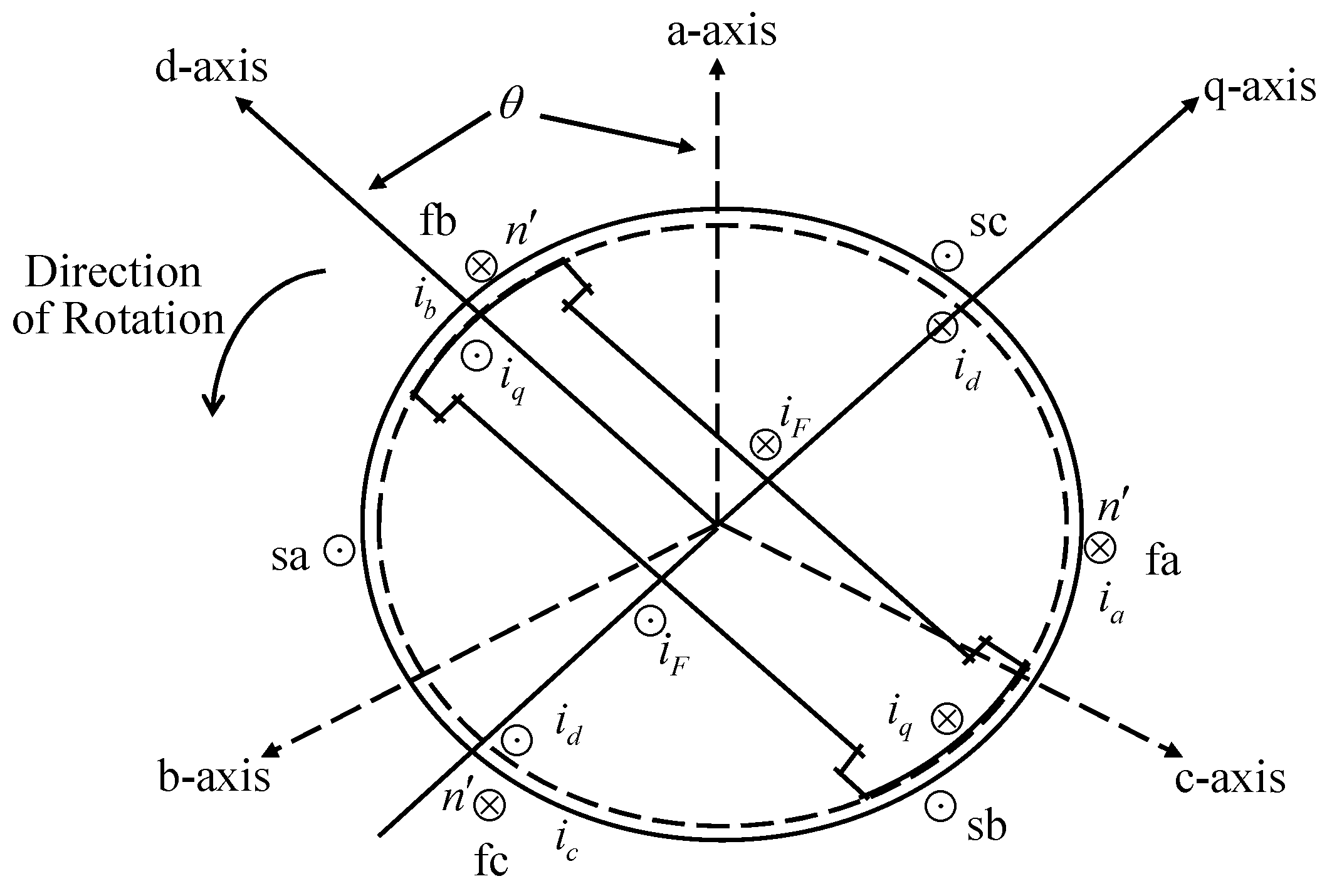
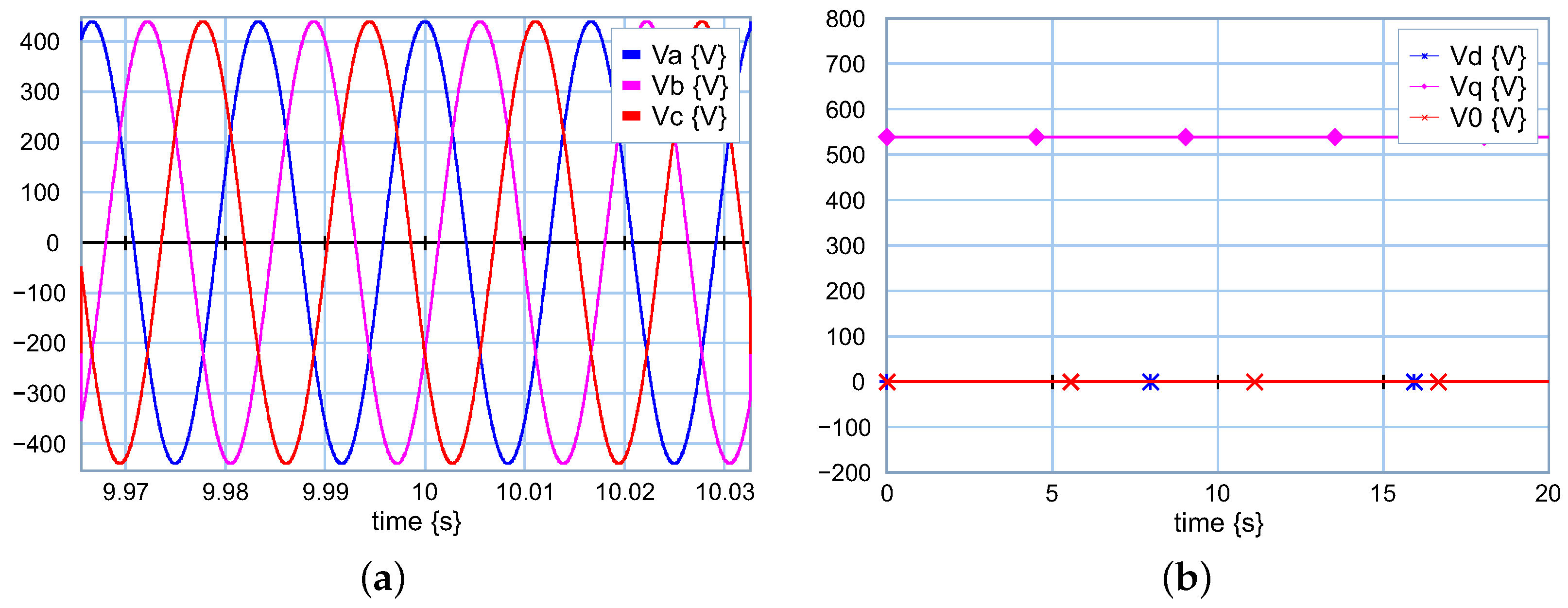
4.1. Synchronous Generator

Currently, the majority of electrical power systems are based on the generation of electrical energy in hydroelectric, thermoelectric and nuclear power plants, which have synchronous generators as their main element [24,25,26]. A diagram of a two-pole synchronous generator is shown in Figure 14. This machine is characterized by having a three-phase armature winding $\left(a,b,c\right)$ as a stator; in the rotor, the field winding $\left(f\right)$ causes excitation; and a damping winding eliminates electromagnetic transients $\left(D,Q\right)$.

Figure 14. Schematic diagram of a three-phase synchronous generator.

Figure 15 illustrates the equivalent circuits of the synchronous generator where the armature winding is indicated, which is represented by three lines with resistance and inductance equivalent to each phase $\left(R_a,L_a\right)$, $\left(R_b,L_b\right)$ and $\left(R_c,L_c\right)$; the field winding is a circuit with a DC voltage source with its equivalent resistance and inductance $\left(R_f,L_f\right)$, and the damping winding is modeled as two shorted circuits with resistance and inductance $\left(R_D,L_D\right)$ and $\left(R_Q,L_Q\right)$, respectively.

Figure 15. Stator and rotor circuits of a synchronous generator.

The model of the synchronous generator with its armature winding determines a time-varying three-phase electrical subsystem. Due to this, the Park transformation is applied to have a coordinate transformation and obtain an equivalent time-invariant system.

The following assumptions are considered to obtain the generator model:

• The stator windings are sinusoidally distributed along the air gap.
• The inductance of the rotor with its position does not cause variation due to stator slots.
• The phenomena of hysteresis and magnetic saturation are not taken into account.

From Figure 15, the following elements are identified:

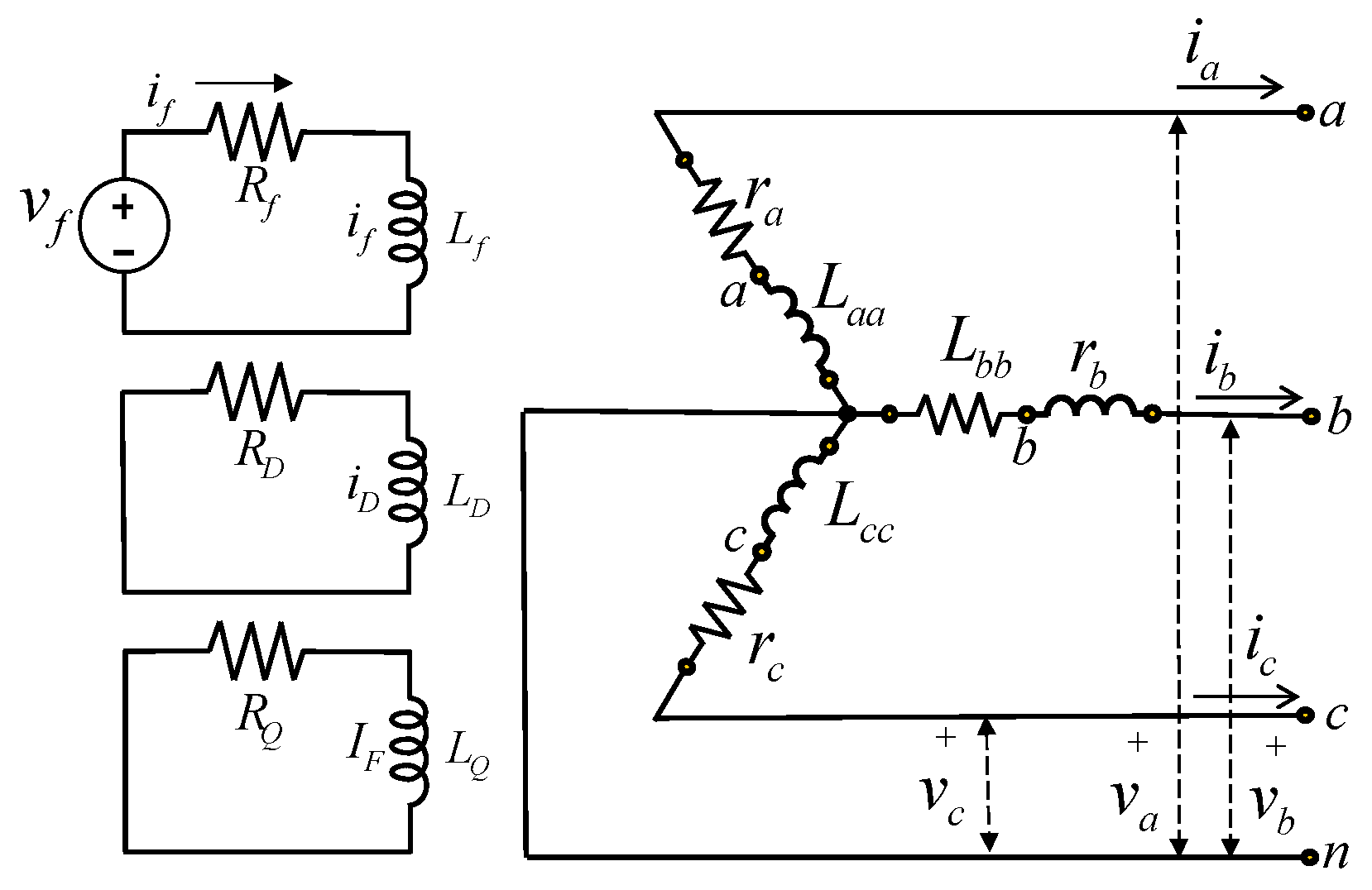
• The armature phase windings are $a,b,c$ with phase voltages and currents $\left(v_a,v_b,v_c\right)$ and $\left(i_a,i_b,i_c\right)$, respectively; $\left(R_a,R_b,R_c\right)$ denote the stator phase resistances, and $\left(L_{aa},L_{bb},L_{cc}\right)$ denote the stator phase self inductances.
• The field winding is f with voltage $v_f$ and current $i_f$ in this winding; $R_f$ and $L_f$ denote resistance and self inductance of this winding, respectively.
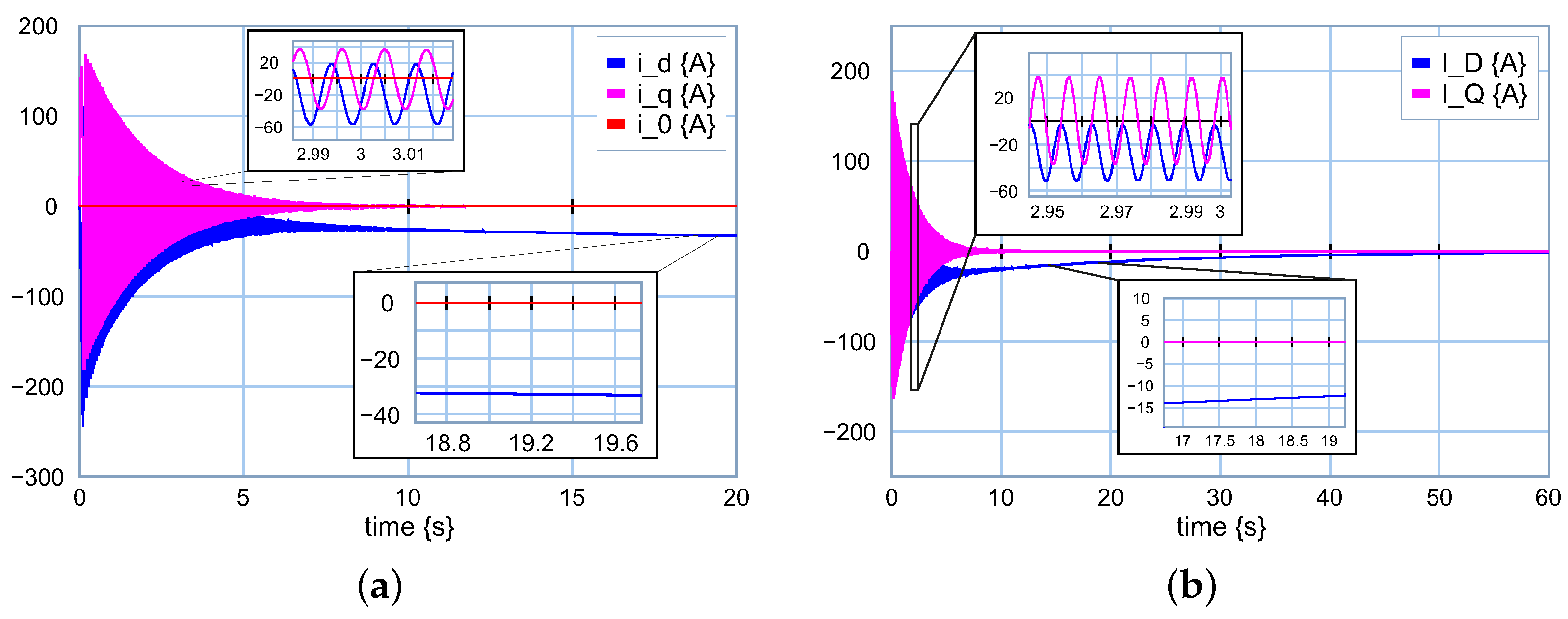
• The damping circuit on the d-axis is D with voltage and current denoted by $v_D$ and $i_D$, respectively; $R_D$ and $L_D$ denote the resistance and self inductance of this winding, respectively.
• The damping circuit on the q-axis is Q with voltage and current denoted by $v_Q$ and $i_Q$, respectively; $R_Q$ and $L_Q$ denote the resistance and self inductance of this winding, respectively.

The synchronous generator of Figure 15 is represented by six windings that are magnetically coupled. The magnetic coupling between the windings is a function of the rotor position. The instantaneous terminal voltage v of any winding is in the form

$$v\left(t\right)=\pm \sum Ri\left(t\right)\pm \stackrel{•}{\lambda }\left(t\right)$$

(94)

where $\lambda \left(t\right)$ is the flux linkage, R is the winding resistance, and $i\left(t\right)$ is the current, with positive directions of stator currents flowing out of the generator terminals.

In order to remove the time variance of the armature winding variables $\left(a,b,c\right)$, the Park transformation is applied so that the new variables in coordinates $\left(d,q,0\right)$ move at the rotor speed. This transformation is defined by [25]

$$i_{dq0}=P{i}_{abc}$$

(95)

where the current vectors are defined as

$$i_{dq0}=\left[\begin{array}{c}{i}_d\\ i_q\\ i_0\end{array}\right];i_{abc}=\left[\begin{array}{c}{i}_a\\ i_b\\ i_c\end{array}\right]$$

(96)

and the Park transformation matrix is

$$P=\sqrt{\frac{2}{3}}\left[\begin{array}{ccc}cos\theta & cos\left(\theta -\frac{2\pi }{3}\right)& cos\left(\theta +\frac{2\pi }{3}\right)\\ sin\theta & sin\left(\theta -\frac{2\pi }{3}\right)& sin\left(\theta +\frac{2\pi }{3}\right)\\ \frac{1}{\sqrt{2}}& \frac{1}{\sqrt{2}}& \frac{1}{\sqrt{2}}\end{array}\right]$$

(97)

The angle between the d-axis and the rotor is described by

$$\theta =w_{R}t+\delta +\frac{\pi }{2}$$

(98)

where $w_R$ is the rated angular frequency in $\mathrm{rad}/\mathrm{s}$, and $\delta$ is the synchronous torque angle in electrical radians.

Similarly, the transformations for voltages and flux links are expressed by

$$\begin{array}{ccc}\hfill v_{dq0}& =& P{v}_{abc}\hfill \end{array}$$

(99)

$$\begin{array}{ccc}\hfill {\lambda }_{dq0}& =& P{\lambda }_{abc}\hfill \end{array}$$

(100)

According to Figure 15, a model ($MBG$-$BG$) of the synchronous generator in coordinates $\left(d,q,0\right)$ is proposed in Figure 16.

Figure 16. ($MBG$-$BG$) of the synchronous generator.

This model has the following characteristics:

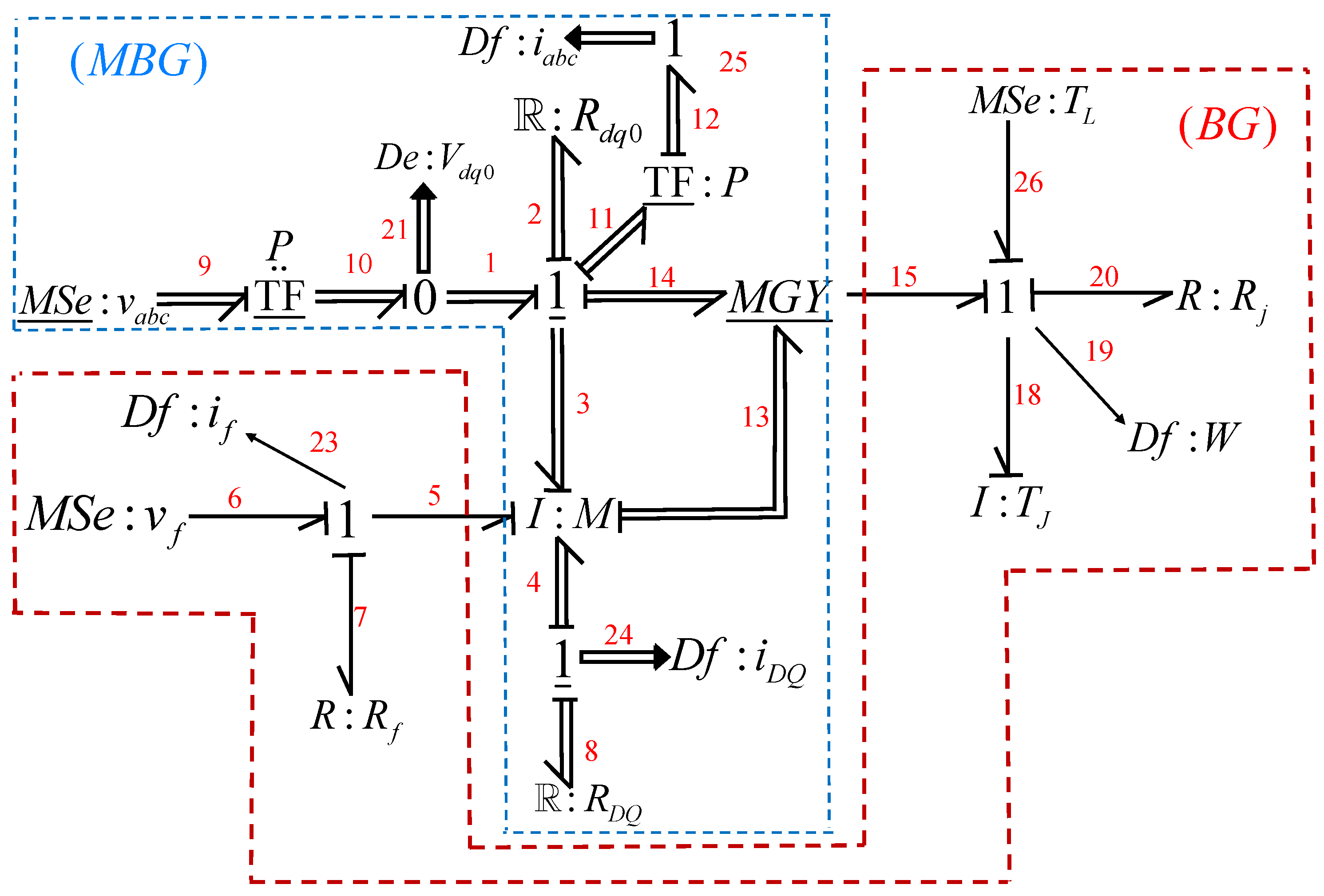
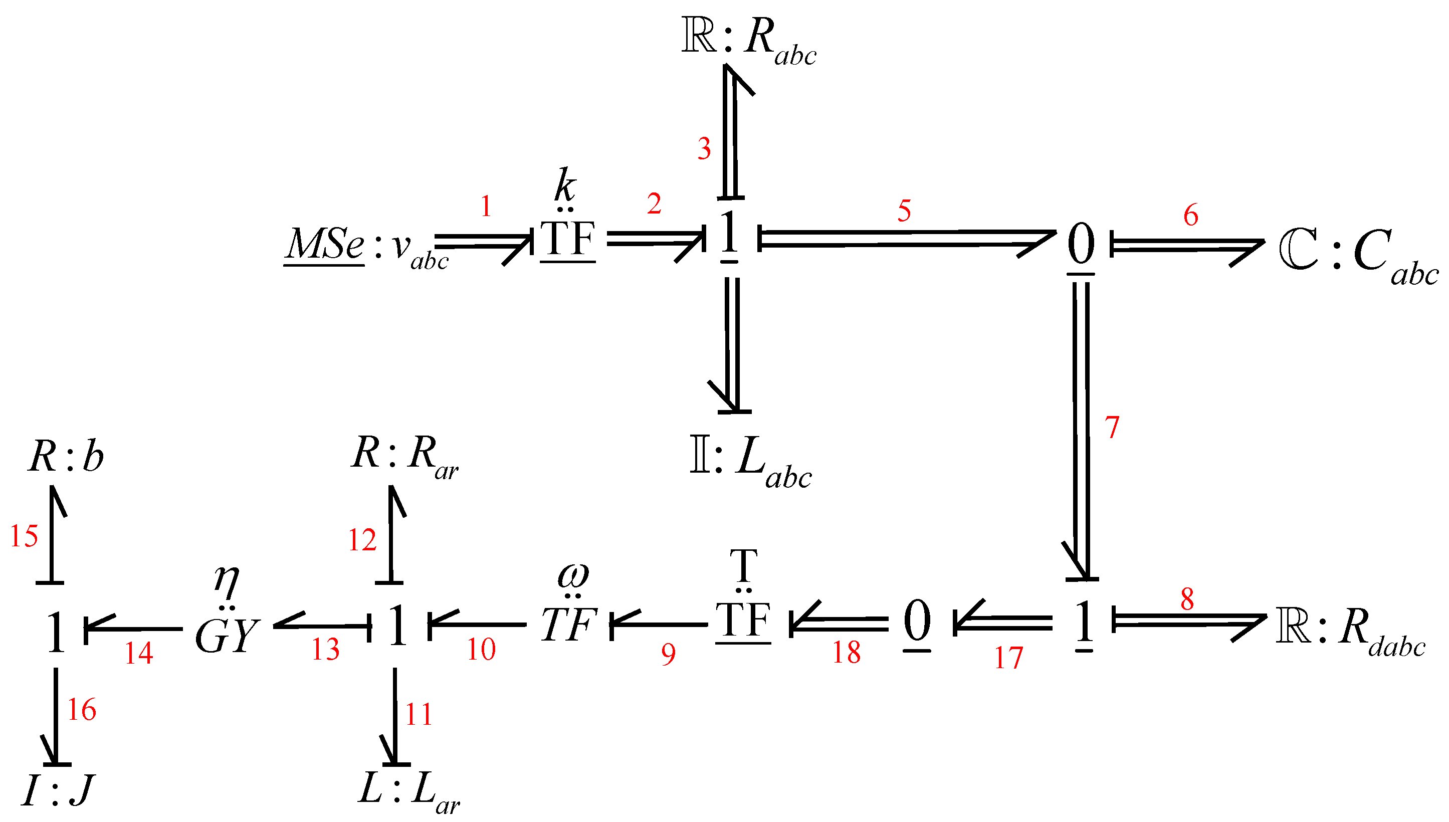
• The section of the armature winding is in coordinates $\left(d,q,0\right)$, to which the multiport resistor $\mathbb{R}:R_{dq0}$ with multibond 2 and multiport inductance $II:L_{dq0}$ with multibond 3 are connected. The multiport effort source 17 in coordinates $\left(a,b,c\right)$ is connected to a multiport transformer $\underline{TF}$ modulated with the Park transformation matrix so that the multibond 10 has a multiport effort equivalent to the voltage in coordinates $\left(d,q,0\right)$. The multibond 14 is the stator–rotor connection in a synchronous generator through a multiport gyrator $\underline{MGY}$ modulated by a matrix T, which are the flux links ${\lambda }_d$ and ${\lambda }_q$ that give rise to the electromagnetic torque of the machine. Note that the multibonds in this section are dimension 3.
• The section of the damping windings are used in a synchronous generator to start the machine and as a means of energy dissipation when there are internal or external electromagnetic transients to the machine. These windings are modeled on the rotor as two shorted windings for which the multiport resistance is $\mathbb{R}:R_{DQ}$, which is connected to bond 8. These windings have their self- and mutual-inductance with respect to the inductances of the other windings of the machine, so this inductance is $II:L_{DQ}$. These windings have no supply source, and note that these multibonds are dimension 2.
• The last electrical section of this generator is constituted by the field winding $R:R_F$ of bond 7 and is linked by bond 5 to the inductance of this winding $I:L_F$. Note that the dimension of this section is 1.
• The mechanical section consists of the moment of inertia of the generator $I:T_j$ connected to bond 18. Considering the effects of air friction with mechanical resistance $R:R_j$ with bond 20, the mechanical energy input to the generator is through the effort source $M{S}_e:T_m$ linked to bond 16. The conversion of mechanical energy to electrical energy is carried out by means of the multiport gyrator $\underline{MGY}$, for which bond 17 is the mechanical part of dimension 1, and the electrical part is multibond 19 of dimension 3 since it determines the three-phase electrical generation.
• The subsystems of the multiport armature winding $\left(d,q,0\right)$ of dimension 3, of the damping windings $\left(D,Q\right)$ of dimension 2, and of the field winding $\left(F\right)$ of dimension 1 due to the design and construction structure of the generator present mutual magnetic flux links and determine mutual inductances $M_{dD}$, $M_{dF}$, $M_{qQ}$, $M_{DF}$, $M_{Dd}$, $M_{Fd},$ $M_{Qq}$ and $M_{FD}$. Therefore, they are modeled in a multiport field $II:M$ in which the self- and mutual-inductances of these windings are considered.

The key vectors of the multibond graph–bond graph model ($MBG$-$BG$) of the generator for the storage elements are defined by

$$\begin{array}{ccc}\hfill \underline{x}\left(t\right)& =& \left[\begin{array}{c}\underline{p_3}\\ \underline{p_4}\end{array}\right];\stackrel{•}{\underline{x}}\left(t\right)=\left[\begin{array}{c}\underline{e_3}\\ \underline{e_4}\end{array}\right];\underline{z}\left(t\right)=\left[\begin{array}{c}\underline{f_3}\\ \underline{f_4}\end{array}\right]\hfill \end{array}$$

(101)

$$\begin{array}{ccc}\hfill x\left(t\right)& =& \left[\begin{array}{c}{p}_5\\ p_{18}\end{array}\right];\stackrel{•}{x}\left(t\right)=\left[\begin{array}{c}{e}_5\\ e_{18}\end{array}\right];z\left(t\right)=\left[\begin{array}{c}{f}_5\\ f_{18}\end{array}\right]\hfill \end{array}$$

(102)

where the constitutive relations are given by

$$\left[\begin{array}{c}\underline{f_3}\\ \underline{f_4}\\ f_5\\ f_{18}\end{array}\right]={\left[\begin{array}{cc}\mathbf{F}& {\mathbf{F}}_m\\ {\mathbf{F}}_m^T& F\end{array}\right]}^{-1}\left[\begin{array}{c}\underline{p_3}\\ \underline{p_4}\\ p_5\\ p_{18}\end{array}\right]$$

(103)

where

$${\mathbf{F}}^{-1}=\left[\begin{array}{cc}{L}_{dq0}& M_{34}\\ M_{34}^T& L_{DQ}\end{array}\right];{\mathbf{F}}_m^{-1}=\left[\begin{array}{cc}{M}_{35}& 0\\ M_{45}& 0\end{array}\right];F^{-1}=\left[\begin{array}{cc}{L}_F& 0\\ 0& T_j\end{array}\right]$$

(104)

with

$$\begin{array}{ccc}\hfill L_{dq0}& =& diag\left\{L_d,L_q,L_0\right\}\hfill \end{array}$$

(105)

$$\begin{array}{ccc}\hfill L_{DQ}& =& diag\left\{L_D,L_Q\right\}\hfill \end{array}$$

(106)

$$\begin{array}{ccc}\hfill M_{34}& =& \left[\begin{array}{cc}{M}_{dD}& 0\\ 0& M_{qQ}\\ 0& 0\end{array}\right];M_{35}=\left[\begin{array}{c}{M}_{dF}\\ 0\\ 0\end{array}\right];M_{45}=\left[\begin{array}{c}{M}_{DF}\\ 0\end{array}\right]\hfill \end{array}$$

(107)

The key vectors for the dissipation elements

$$\begin{array}{ccc}\hfill \underline{D_{in}}\left(t\right)& =& \left[\begin{array}{c}\underline{f_2}\\ \underline{f_8}\end{array}\right];\underline{D_{out}}\left(t\right)=\left[\begin{array}{c}\underline{e_2}\\ \underline{e_8}\end{array}\right]\hfill \end{array}$$

(108)

$$\begin{array}{ccc}\hfill D_{in}\left(t\right)& =& \left[\begin{array}{c}{f}_7\\ f_{20}\end{array}\right];D_{out}\left(t\right)=\left[\begin{array}{c}{e}_7\\ e_{20}\end{array}\right]\hfill \end{array}$$

(109)

with constitutive relations given by

$$\begin{array}{ccc}\hfill \mathbf{L}& =& diag\left\{R_{dq0},R_{DQ}\right\}\hfill \end{array}$$

(110)

$$\begin{array}{ccc}\hfill L& =& diag\left\{R_F,R_j\right\}\hfill \end{array}$$

(111)

with

$$\begin{array}{ccc}\hfill R_{dq0}& =& diag\left\{R_d,R_q,R_0\right\}\hfill \end{array}$$

(112)

$$\begin{array}{ccc}\hfill R_{DQ}& =& diag\left\{R_D,R_Q\right\}\hfill \end{array}$$

(113)

The inputs to the system are

$$\underline{u}\left(t\right)=\underline{e_9};u\left(t\right)=\left[\begin{array}{c}{e}_6\\ e_{16}\end{array}\right]$$

(114)

and the selected outputs are the currents in coordinates $\left(a,b,c\right)$, defined by

$$\underline{y}\left(t\right)=\underline{f_{12}}$$

(115)

The multiport junction structure is described by

$$\left[\begin{array}{c}\underline{e_3}\\ \underline{e_4}\\ ine{e}_5\\ e_{18}\\ ineine\underline{f_2}\\ \underline{f_8}\\ ine{f}_7\\ f_{20}\\ ine{f}_{12}\end{array}\right]=\left[\begin{array}{ccccccccccccc}\mathbf{0}& \mathbf{0}& \mathbf{0}& -T& & -I& \mathbf{0}& \mathbf{0}& \mathbf{0}& & P^{-1}& \mathbf{0}& \mathbf{0}\\ \mathbf{0}& \mathbf{0}& \mathbf{0}& \mathbf{0}& & \mathbf{0}& -I& \mathbf{0}& \mathbf{0}& & \mathbf{0}& \mathbf{0}& \mathbf{0}\\ ine0& 0& 0& 0& & 0& 0& -1& 0& & 0& 1& 0\\ T^T& 0& 0& 0& & 0& 0& 0& -1& & 0& 0& 1\\ ineineI& \mathbf{0}& \mathbf{0}& \mathbf{0}& & \mathbf{0}& \mathbf{0}& \mathbf{0}& \mathbf{0}& & \mathbf{0}& \mathbf{0}& \mathbf{0}\\ \mathbf{0}& I& \mathbf{0}& \mathbf{0}& & \mathbf{0}& \mathbf{0}& \mathbf{0}& \mathbf{0}& & \mathbf{0}& \mathbf{0}& \mathbf{0}\\ ine0& 0& 1& 0& & 0& 0& 0& 0& & 0& 0& 0\\ 0& 0& 0& 1& & 0& 0& 0& 0& & 0& 0& 0\\ ineP& 0& 0& 0& & 0& 0& 0& 0& & 0& 0& 0\end{array}\right]\left[\begin{array}{c}\underline{f_3}\\ \underline{f_4}\\ ine{f}_5\\ f_{18}\\ ineine\underline{e_2}\\ \underline{e_8}\\ ine{e}_7\\ e_{20}\\ ineine\underline{e_1}\\ ine{e}_6\\ e_{16}\end{array}\right]$$

(116)

where

$$T^T=\left[\begin{array}{ccc}{\lambda }_q& -{\lambda }_d& 0\end{array}\right]$$

In order to obtain the mathematical model of the system in state space, the proposed lemma is applied. As there are no storage elements in derivative causality,

$$\mathbf{E}\left(\underline{x}\right)=\left[\begin{array}{cc}\mathbf{I}& \mathbf{0}\\ \mathbf{0}& I\end{array}\right]$$

(117)

Likewise, there are no algebraic loops in both sections of the multibond graph and bond graph

$$\begin{array}{ccc}\hfill \mathbf{M}\left(\underline{x}\right)& =& \mathbf{L}\hfill \end{array}$$

(118)

$$\begin{array}{ccc}\hfill M\left(x\right)& =& L\hfill \end{array}$$

(119)

From (56) and (57) with (110), (111), (116), (118) and (119),

$$\begin{array}{ccc}\hfill {\mathbf{A}}_{11}^{\prime }\left(\underline{x}\right)& =& \left[\begin{array}{cc}-R_{dq0}& 0\\ 0& -R_{DQ}\end{array}\right]\hfill \end{array}$$

(120)

$$\begin{array}{ccc}\hfill {\mathbf{A}}_{12}^{\prime }\left(\underline{x}\right)& =& \left[\begin{array}{cc}0& -T\\ 0& 0\end{array}\right]\hfill \end{array}$$

(121)

From the first line of (55),

$$\begin{array}{ccc}\hfill {\mathbf{A}}_{11}\left(\underline{x}\right)& =& -\left[\begin{array}{cc}{R}_{dq0}L{\prime }_{dq0}& R_{dq0}M{\prime }_{34}\\ R_{DQ}\left(M_{34}^T\right)\prime & R_{DQ}L{\prime }_{DQ}\end{array}\right]\hfill \end{array}$$

(122)

$$\begin{array}{ccc}\hfill {\mathbf{A}}_{12}\left(\underline{x}\right)& =& -\left[\begin{array}{cc}{R}_{dqo}M{\prime }_{35}& -T·T_j\\ R_{DQ}M{\prime }_{45}& 0\end{array}\right]\hfill \end{array}$$

(123)

where

$${\left[\begin{array}{ccc}{L}_{dq0}& M_{34}& M_{35}\\ M_{34}^T& L_{DQ}& M_{45}\\ M_{35}^T& M_{45}^T& L_F\end{array}\right]}^{-1}=\left[\begin{array}{ccc}L{\prime }_{dq0}& M{\prime }_{34}& M{\prime }_{35}\\ \left(M_{34}^T\right)\prime & L{\prime }_{DQ}& M{\prime }_{45}\\ \left(M_{35}^T\right)\prime & \left(M_{45}^T\right)\prime & L{\prime }_F\end{array}\right]$$

(124)

From (60)–(62) with (116), (118) and (119), the multiport input matrix is defined by

$$\begin{array}{ccc}\hfill {\mathbf{B}}_{11}\left(\underline{x}\right)& =& \left[\begin{array}{c}{P}^{-1}\\ 0\end{array}\right]\hfill \end{array}$$

(125)

$$\begin{array}{ccc}\hfill {\mathbf{B}}_{12}\left(\underline{x}\right)& =& \left[\begin{array}{c}0\\ 0\end{array}\right]\hfill \end{array}$$

(126)

From (58), (110), (111), (116), (118) and (119),

$$A_{21}^{\prime }\left(\underline{x}\right)=\left[\begin{array}{cc}0& 0\\ T^T& 0\end{array}\right]$$

(127)

From (59), (110), (111), (116), (118) and (119),

$$A_{22}^{\prime }\left(\underline{x}\right)=\left[\begin{array}{cc}-R_F& 0\\ 0& -R_j\end{array}\right]$$

(128)

From the second line of (55),

$$\begin{array}{ccc}\hfill A_{21}\left(\underline{x}\right)& =& \left[\begin{array}{cc}-R_{F}M{\prime }_{35}& -R_{F}M{\prime }_{45}\\ T^{T}L{\prime }_{dq0}& 0\end{array}\right]\hfill \end{array}$$

(129)

$$\begin{array}{ccc}\hfill A_{22}\left(\underline{x}\right)& =& \left[\begin{array}{cc}-R_{F}L{\prime }_F& 0\\ T^{T}M{\prime }_{35}& -R_{j}T{\prime }_j\end{array}\right]\hfill \end{array}$$

(130)

The input matrix is obtained from (63), (64), (116), (118) and (119)

$$\begin{array}{ccc}\hfill B_{21}\left(\underline{x}\right)& =& 0\hfill \end{array}$$

(131)

$$\begin{array}{ccc}\hfill B_{22}\left(\underline{x}\right)& =& I\hfill \end{array}$$

(132)

By substituting (122), (123), (125) and (126) into the first line of (53) with (55), the state equation for the multibond graph section in a three coordinates is defined

$$\stackrel{•}{\underline{x}}\left(t\right)=-\left[\begin{array}{cc}{R}_{dq0}L{\prime }_{dq0}& R_{dq0}M{\prime }_{34}\\ R_{DQ}\left(M_{34}^T\right)\prime & R_{DQ}L{\prime }_{DQ}\end{array}\right]\underline{x}\left(t\right)-\left[\begin{array}{cc}{R}_{dqo}M{\prime }_{35}& -T·T_j\\ R_{DQ}M{\prime }_{45}& 0\end{array}\right]x\left(t\right)+\left[\begin{array}{c}{P}^{-1}\\ 0\end{array}\right]\underline{u}\left(t\right)$$

(133)

And substituting (129)–(132) into the second line of (53) with the second lines of (55) and (60),

$$\stackrel{•}{x}\left(t\right)=\left[\begin{array}{cccc}-R_{F}M{\prime }_{35}& -R_{F}M{\prime }_{45}& -R_{F}L{\prime }_F& 0\\ T^{T}L{\prime }_{dq0}& 0& T^{T}M{\prime }_{35}& -R_{j}T{\prime }_j\end{array}\right]\left[\begin{array}{c}\underline{x}\left(t\right)\\ x\left(t\right)\end{array}\right]+\left[\begin{array}{ccc}0& 1& 0\\ 0& 0& 1\end{array}\right]\left[\begin{array}{c}\underline{e_1}\\ e_6\\ e_{16}\end{array}\right]$$

(134)

From (69), (70), (74) and (75) with the first line of (68) and (73), the output equation is given by

$$\underline{y}\left(t\right)=\left[\begin{array}{cccc}P& 0& 0& 0\end{array}\right]\left[\begin{array}{c}\underline{x}\left(t\right)\\ x\left(t\right)\end{array}\right]$$

(135)

With the state equations given by (133) and (134), we have the representation of a system modeled by multibond graphs and bond graphs. In addition, there are the terms due to $\left(MBG\right)$, the terms of $\left(BG\right)$, and also the relationship between them.

In order to obtain the behavior of the synchronous generator using the ($MBG$-$BG$) model, simulation results using 20-Sim software are shown. The numerical parameters of the generator elements are indicated in Table 2.

Table 2. Parameters of the case study.

${\mathit{v}}_{\mathit{a}}=440sin\left(\mathit{w}\mathit{t}\right)$ V	${\mathit{R}}_{\mathit{d}}=0.1$ $\Omega$	${\mathit{L}}_{\mathit{d}}=1.7\mathit{H}$	${\mathit{M}}_{\mathit{d}\mathit{D}}=1.55\mathit{H}$
$v_b=440sin\left(wt-2\pi /3\right)$ V	$R_q=0.1$ $\Omega$	$L_q=1.64H$	$M_{qQ}=1.49H$
$v_c=440sin\left(wt+2\pi /3\right)$ V	$R_0=1.0$ $\Omega$	$L_0=1.0H$	$M_{dF}=1.55H$
$v_F=120$ V	$R_F=2.5$ $\Omega$	$L_D=1.605H$	$M_{DF}=1.55H$
$T_m=1000$ N·m	$R_J=1.0$ N·m·s	$L_Q=1.526H$	$T_J=2.37$ N·m·s${}^2$

The first part of the simulation results consists of the three-phase supply voltages to the generator in coordinates $\left(a,b,c\right)$ and in coordinates $\left(d,q,0\right)$ as shown in Figure 17.

Figure 17. Supply voltages: (a) in coordinates $\left(a,b,c\right)$; (b) in coordinates $\left(d,q,0\right)$.

The three-phase voltage applied to the generator is in balanced conditions: that is, it is at a constant maximum magnitude and with a phase shift of 120 in coordinates $\left(a,b,c\right)$, defining voltages of constant magnitude in coordinates $\left(d,q,0\right)$.

The response of the ($MBG$-$BG$) model is found with the currents $\left(i_d,i_q,i_0\right)$, which is the response of the generator when the three-phase voltages are supplied; the torque applied to the mechanical subsection indicates the input mechanical energy and is related to the voltage in the excitation winding. Thus, the currents $\left(i_d,i_q,i_0\right)$ shown in Figure 18a are stable after the transient period has finished. These current signals are obtained from the multibond graph with multibonds of dimension 3.

Figure 18. Electric currents of the model: (a) of the main windings in coordinates $\left(d,q,0\right)$; (b) of the damping windings $\left(D,Q\right)$.

Figure 18b shows the currents in the damping windings $\left(i_D,i_Q\right)$, which absorb the energy of the electromechanical transient of the generator at its startup and which after the dynamic period must stabilize at zero magnitude as seen in the corresponding graphs. These currents are obtained from the multibond graph with multibonds of dimension 2.

Figure 19 shows the two remaining variables of the generator model, which are the current in the excitation winding $i_F$ and the speed w; both signals being stable indicates good operation of the generator. These excitation current and velocity signals are obtained from the bond graph part of the model with bonds of dimension 1.

Figure 19. (a) Current in the field winding and (b) speed.

Finally, the objective of the generator is to supply electrical energy to the system through the currents $\left(i_a,i_b,i_c\right)$ that are obtained from the currents $\left(i_d,i_q,i_0\right)$; the section representing these currents in the multibond graph indicates that balanced three-phase currents are delivered to the system, showing good operation of the generator, which is shown in Figure 20.

Figure 20. Output current in coordinates $\left(a,b,c\right)$.

4.2. Three-Phase Electrical System

Electrical power systems allow the generation, transmission, distribution and consumption of electrical energy. This case study consists of a three-phase electrical energy generation system $\left(v_a,v_{b,}{v}_c\right)$ Figure 21 present the second case study. Due to the difference in the generation and transmission voltage levels, a set of single-phase transformers $\left(T_1,T_2,T_3\right)$ is connected between the supply and the transmission lines formed by the resistance and inductance connected to phase $a:\left(R_a,L_a\right)$, phase $b:\left(R_b,L_b\right)$ and phase $c:\left(R_c,L_c\right)$. These lines are connected to an energy storage system made up of capacitors $\left(C_a,C_b,C_c\right)$. From the terminals of the capacitors, it is necessary to connect a DC motor, for which a three-phase rectifier $\left(D_a,D_b,D_c\right)$ based on power diodes is applied. The output of this rectifier feeds a motor through a single-phase transformer $\left(T_4\right)$ to guarantee that the motor receives the voltage at its terminals at the desired value.

Figure 21. Electrical power system feeding a DC motor.

The DC motor model consists of the resistance $R_{ar}$ and inductance $L_{ar}$ armature winding parameters; the mechanical part of the motor is formed by the inertia J and friction with the air b; the electromechanical conversion takes place with a module n. For this motor, the field winding is constant, so its model is not necessary. The complete model of this system is shown in Figure 22.

Figure 22. ($MBG$-$BG$) of the electrical power system.

A fundamental aspect of modeling systems with multibond graphs and bond graphs is to be able to link these and make them graphically and mathematically consistent. Therefore, for the output of the three-phase rectifier and the input to the single-phase transformer $\left(T_4\right)$, another transformer with a $\left(T\right)$ module is required to make this connection. Note that the three-phase rectifier is modeled based on nonlinear resistances $R_{dabc}$ of the Schottky model.

The key vectors are defined by

$$\begin{array}{ccc}\hfill \underline{x}\left(t\right)& =& \left[\begin{array}{c}\underline{p_4}\\ \underline{q_6}\end{array}\right];\stackrel{•}{\underline{x}}\left(t\right)=\left[\begin{array}{c}\underline{e_4}\\ \underline{f_6}\end{array}\right];\underline{z}\left(t\right)=\left[\begin{array}{c}\underline{f_4}\\ \underline{e_6}\end{array}\right]\hfill \end{array}$$

(136)

$$\begin{array}{ccc}\hfill x\left(t\right)& =& \left[\begin{array}{c}{p}_{11}\\ p_{16}\end{array}\right];\stackrel{•}{x}\left(t\right)=\left[\begin{array}{c}{e}_{11}\\ e_{16}\end{array}\right];z\left(t\right)=\left[\begin{array}{c}{f}_{11}\\ f_{16}\end{array}\right]\hfill \end{array}$$

(137)

with the constitutive relationships of these storage elements expressed by

$$\mathbf{F}=diag\left\{L_{abc}^{-1},C_{abc}^{-1}\right\}$$

(138)

where

$$\begin{array}{ccc}\hfill L_{abc}& =& \left[\begin{array}{ccc}{l}_a& l_{ab}& l_{ac}\\ l_{ab}& l_b& l_{bc}\\ l_{ac}& l_{bc}& l_c\end{array}\right]\hfill \end{array}$$

(139)

$$\begin{array}{ccc}\hfill C_{abc}& =& \left[\begin{array}{ccc}{c}_a& 0& 0\\ 0& c_b& 0\\ 0& 0& c_c\end{array}\right]\hfill \end{array}$$

(140)

The key vectors for the dissipative elements are defined by

$$\begin{array}{ccc}\hfill \underline{D_{in}}\left(t\right)& =& \left[\begin{array}{c}\underline{f_3}\\ \underline{f_8}\end{array}\right];\underline{D_{out}}\left(t\right)=\left[\begin{array}{c}\underline{e_3}\\ \underline{e_8}\end{array}\right]\hfill \end{array}$$

(141)

$$\begin{array}{ccc}\hfill D_{in}\left(t\right)& =& \left[\begin{array}{c}{f}_{12}\\ f_{15}\end{array}\right];D_{out}\left(t\right)=\left[\begin{array}{c}{e}_{12}\\ e_{15}\end{array}\right]\hfill \end{array}$$

(142)

with the constitutive relations

$$\begin{array}{ccc}\hfill \mathbf{L}& =& diag\left\{R_{abc},R_{dabc}\right\}\hfill \end{array}$$

(143)

$$\begin{array}{ccc}\hfill L& =& diag\left\{R_{ar},b\right\}\hfill \end{array}$$

(144)

with the input

$$\underline{u}\left(t\right)=\underline{e_1}$$

(145)

The input and output relations of the transformer with module T are given by

$$\begin{array}{ccc}\hfill e_9& =& T\underline{e_{18}}\hfill \end{array}$$

(146)

$$\begin{array}{ccc}\hfill \underline{e_{18}}& =& T^T{e}_9\hfill \end{array}$$

(147)

where

$$T=\left[\begin{array}{ccc}1& 1& 1\end{array}\right]$$

(148)

The junction structure of ($MBG$-$BG$) is given by

$$\left[\begin{array}{c}\underline{e_4}\\ \underline{f_6}\\ ine{e}_{11}\\ e_{16}\\ ineine\underline{f_3}\\ \underline{f_8}\\ ine{f}_{12}\\ f_{15}\end{array}\right]=\left[\begin{array}{ccccccccccc}\mathbf{0}& -\mathbf{I}& \mathbf{0}& \mathbf{0}& & -\mathbf{I}& \mathbf{0}& \mathbf{0}& \mathbf{0}& & K^{-1}\\ \mathbf{I}& \mathbf{0}& \frac{-1}{w}{T}^T& \mathbf{0}& & \mathbf{0}& 0& 0& 0& & 0\\ ine0& \frac{1}{w}T& 0& -n& & 0& \frac{-1}{w}T& -1& 0& & 0\\ 0& 0& n& 0& & 0& 0& 0& -1& & 0\\ ineine\mathbf{I}& \mathbf{0}& \mathbf{0}& \mathbf{0}& & \mathbf{0}& \mathbf{0}& \mathbf{0}& \mathbf{0}& & \mathbf{0}\\ \mathbf{0}& \mathbf{0}& \frac{1}{w}T& \mathbf{0}& & \mathbf{0}& \mathbf{0}& \mathbf{0}& \mathbf{0}& & \mathbf{0}\\ ine0& 0& 1& 0& & 0& 0& 0& 0& & 0\\ 0& 0& 0& 1& & 0& 0& 0& 0& & 0\end{array}\right]\left[\begin{array}{c}\underline{f_4}\\ \underline{e_6}\\ ine{f}_{11}\\ f_{16}\\ ineine\underline{e_3}\\ \underline{e_8}\\ ine{e}_{12}\\ e_{15}\\ ineine\underline{e_1}\end{array}\right]$$

(149)

In this case, $S_{22}^{11}\left(x\right)=0$ and $S_{22}^{22}\left(x\right)=0$; then (65) and (66)

$$\begin{array}{ccc}\hfill \mathbf{M}\left(\underline{x}\right)& =& \mathbf{L}\hfill \end{array}$$

(150)

$$\begin{array}{ccc}\hfill M\left(x\right)& =& L\hfill \end{array}$$

(151)

Also, there are no storage elements in derivative causality; then $\mathbf{E}\left(\underline{x}\right)=\mathbf{I}$.

From (56), (150) and (151) with (143), (144) and (149),

$${\mathbf{A}}_{11}^{\prime }\left(\underline{x}\right)=\left[\begin{array}{cc}-R_{abc}& -I\\ I& 0\end{array}\right]$$

(152)

From (57), (150) and (151) with (149),

$${\mathbf{A}}_{12}^{\prime }\left(\underline{x}\right)=\left[\begin{array}{cc}0& 0\\ \frac{-1}{w}{T}^T& 0\end{array}\right]$$

(153)

From (58), (150) and (151) with (149),

$$A_{21}^{\prime }\left(\underline{x}\right)=\left[\begin{array}{cc}0& \frac{1}{w}T\\ 0& 0\end{array}\right]$$

(154)

From (59), (150) and (151) with (143), (144) and (149),

$$A_{22}^{\prime }\left(\underline{x}\right)=\left[\begin{array}{cc}-R_{ar}+\frac{1}{w}T{R}_{dabc}{T}^T& 0\\ 0& -b\end{array}\right]$$

(155)

From (61) and (63) with (151), (143), (144) and (149),

$${\mathbf{B}}_{11}\left(\underline{x}\right)=\left[\begin{array}{c}{K}^{-1}\\ 0\end{array}\right]$$

(156)

and

$$B_{21}\left(\underline{x}\right)=\left[\begin{array}{c}0\\ 0\end{array}\right]$$

(157)

For this case study, there are no energy storage element fields, so $F_m=0$. From (55) and (60) with (152)–(157), the state equation given by (53) is defined as

$$\left[\begin{array}{c}\underline{\stackrel{•}{x}}\left(t\right)\\ \stackrel{•}{x}\left(t\right)\end{array}\right]=\left[\begin{array}{cccc}-R_{abc}{L}_{abc}^{-1}& -C_{abc}^{-1}& 0& 0\\ -L_{abc}^{-1}& 0& {\displaystyle \frac{-1}{w{L}_{ar}}}{T}^T& 0\\ 0& {\displaystyle \frac{1}{w}}T{C}_{abc}^{-1}& -{\displaystyle \frac{R_{ar}}{L_{ar}}}+{\displaystyle \frac{1}{w{L}_{ar}}}T{R}_{dabc}{T}^T& 0\\ 0& 0& 0& {\displaystyle \frac{-b}{J}}\end{array}\right]\left[\begin{array}{c}\underline{x}\left(t\right)\\ x\left(t\right)\end{array}\right]+\left[\begin{array}{c}{K}^{-1}\\ 0\\ 0\\ 0\end{array}\right]\underline{u}\left(t\right)$$

(158)

From this paper, structural properties of a model can be obtained. Likewise, the control design in section $\left(BG\right)$ to $\left(MGB\right)$ or the opposite can be established for future work.

5. Conclusions

System modeling with the combination of multibond graphs with bond graphs has been presented. Physical systems such as electrical power, aeronautical and robotic systems, due to their characteristics, require modeling in several axes or dimensions, and at the same time, there are components that are represented in one axis or dimension, so this paper responds to the need to model these systems through ($MBG$-$BG$). The mathematical modeling of systems represented by ($MBG$-$BG$) is proposed through a junction structure that is introduced. Finally, the modeling and simulation of a synchronous generator on the ($MBG$-$BG$) platform has been presented. Additionally, the obtainment of a state-space model of an electrical power system feeding a DC motor is proposed. Structural properties such as stability, controllability and singular perturbations of systems modeled by ($MBG$-$BG$) as future work can be proposed from this paper.

References

- Sueur, C.; Dauphin-Tanguy, G. Bond graph approach for structural analysis of MIMO linear system. J. Frankl. Inst. 1991, 328, 55–70. [Google Scholar] [CrossRef]
- Antic, D.; Vidojkovic, B.; Mladenovic, M. An Introduction to Bond Graph Modelling of Dynamic Systems. In Proceedings of the TELSIKs 99, Nis, Serbia, 13–15 October 1999. [Google Scholar]
- Karnopp, D. Bond Graphs in Control: Physical State Variables and Observers. J. Frankl. Inst. 1979, 308, 219–234. [Google Scholar] [CrossRef]
- Gawthrop, P. Physical Model-based Control: A Bond Graph Approach. J. Frankl. Inst. 1995, 332B, 285–305. [Google Scholar] [CrossRef]
- Brown, F.T. Hamiltonian and Lagrangian Bond Graphs. J. Frankl. Inst. 1991, 328, 809–831. [Google Scholar] [CrossRef]
- Rahmani, A.; Hasan, M.N.; Zak, M. Modelling and Validation of Electric Vehicle Drive Line Architecture using Bond Graph. Test Eng. Manag. 2020, 82, 15154–15167. [Google Scholar]
- Badoud, A.E.; Merahi, F.; Bouamama, B.O.; Mekhilef, S. Bond Graph modeling, design and experimental validation of a photovoltaic/fuel cell/electrolyzer/battery hybrid power system. Int. J. Hydrogen Energy 2021, 46, 24011–24027. [Google Scholar] [CrossRef]
- Zrafi, R.; Ghedira, S.; Besbes, K. A Bond Graph Approach for the Modeling and Simulation of a Buck Converter. J. Low Power Electron. Appl. 2018, 8, 2. [Google Scholar] [CrossRef]
- Mohammed, A.; Sirahbizu, B.; Lemu, H.G. Optimal Rotary Wind Turbine Blade Modeling with Bond Graph Approach for Specific Local Sites. Energies 2022, 15, 6858. [Google Scholar] [CrossRef]
- Breedveld, P.C. Multibond graph elements in physical systems theory. J. Frankl. Inst. 1985, 319, 1–36. [Google Scholar] [CrossRef]
- Breedveld, P.C. Decomposition of multiport elements in a revised multi bond graph notation. J. Frankl. Inst. 1984, 318, 253–273. [Google Scholar] [CrossRef]
- Behzadipour, S.; Khajepour, A. Causality in vector bond graphs and its application to modeling of multi-body dynamic systems. Simul. Model. Pract. Theory 2006, 14, 279–295. [Google Scholar] [CrossRef]
- Nuñez, I.; Breedveld, P.C.; Weustink, P.B.T.; Gonzalez, G. Steady-State power flow analysis of electrical power systems modelled by 2-dimensional multibond graphs. In Proceedings of the International Conference on Integrated Modeling and Analysis in Applied Control and Automation, Bergeggi, Italy, 21–23 September 2015; pp. 39–47. [Google Scholar]
- Boundon, B.; Malburet, F.; Carmona, J.C. Design Methodology of a Complex CKC Mechanical Joint with an Energetic Representation Tool “Multibond Graph”: Application to the Helicopter. In Multibody Dynamics, Computational Methods and Applications; Springer International Publishing: Berlin/Heidelberg, Germany, 2014. [Google Scholar]
- Mishra, N.; Vaz, A. Bond graph modeling of a 3-joint String-Tube Actuanted finger prosthesis. Mech. Mach. 2017, 117, 1–20. [Google Scholar] [CrossRef]
- Pathak, A.K.; Vaz, A. A simplified model for contact mechanics of articular cartilage and mating bones using bond graph. In Proceedings of the 3rd International and 18th National Conference on Machines and Mechanisms, Mumbai, India, 13–15 December 2017. [Google Scholar]
- Mishra, N.; Vaz, A. Development of trajectory and force controllers for 3-joint string- tube actuated finger prosthesis based on bond graph modeling. Mech. Mach. Theory 2020, 146, 103719. [Google Scholar] [CrossRef]
- Gonzalez, G.; Barrera, N.; Ayala, G.; Padilla, A. Modeling and Simulation in Multibond Graphs Applied to Three-Phase Electrical Systems. Appl. Sci. 2023, 13, 5880. [Google Scholar] [CrossRef]
- Rosenberg, R.C.; Andry, A.N. Solvability of Bond Graph Junction Structures with Loops. IEEE Trans. Circuits Syst. 1979, 26, 130–137. [Google Scholar] [CrossRef]
- Rosenberg, R.C.; Moultrie, B. Basis Order for Bond Graph Junction Structures. IEEE Trans. Circuits Syst. 1980, 27, 909–920. [Google Scholar] [CrossRef]
- Rahmani, A.; Dauphin-Tanguy, G. Structural analysis of switching systems modelled by bond graph. Math. Comput. Dyn. Syst. 2010, 12, 235–247. [Google Scholar] [CrossRef]
- Gonzalez, G.; Padilla, A. Quasi-steady-state model of a class of nonlinear singularly perturbed system in bond graph approach. Electr. Eng. 2018, 100, 293–302. [Google Scholar] [CrossRef]
- Breedveld, P.C. Essential gyrators and equivalence rules for 3-port junction structures. J. Frankl. Inst. 1984, 318, 253–273. [Google Scholar] [CrossRef]
- Kundur, J.R. Power System Stability and Control; Mc. Graw-Hill: New York, NY, USA, 1994. [Google Scholar]
- Anderson, P.M. Power System Control and Stability; The Iowa State University Press: Ames, IA, USA, 1977. [Google Scholar]
- Krause, P.C.; Wasynczuk, O.; Sudhoff, S.D. Analysis of Electrical Machinery and Drive Systems; IEEE Press-Wiley-Interscience: Hoboken, NJ, USA, 2002. [Google Scholar]