An Efficient Method for Variable Selection Based on Diagnostic-Lasso Regression

Abstract

In contemporary statistical methods, robust regression shrinkage and variable selection have gained paramount significance due to the prevalence of datasets characterized by contamination and an abundance of variables, often categorized as ‘high-dimensional data’. The Least Absolute Shrinkage and Selection Operator (Lasso) is frequently employed in this context for both the model and selecting variables. However, no one has attempted to apply regression diagnostic measures to Lasso regression, despite its power and widespread practical use. This work introduces a combined Lasso and diagnostic technique to enhance Lasso regression modeling for high-dimensional datasets with multicollinearity and outliers. We utilize a diagnostic Lasso estimator (D-Lasso). The breakdown point of the proposed method is also discussed. Finally, simulation examples and analyses of real data are provided to support the conclusions. The results of the numerical examples demonstrate that the D-Lasso approach performs as well as, if not better than, the robust Lasso method based on the MM-estimator.

1. Introduction

The usual estimators are inapplicable in cases where the matrix $X^{T}X$ is singular. In practice, when estimating ($\mathit{\beta }$) or pursuing variable selection, high empirical correlations between two or a few other covariates (multicollinarity) lead to unstable outcomes. This study uses the least absolute shrinkage and selection operator (Lasso) estimation method in order to circumvent this issue.

Lasso estimation is a type of variable selection. It was first described by Tibshirani [1] and was further studied by Fan and Li [2]. They explored a class of penalized likelihood approaches to address these types of problems, including the Lasso problem.

In contrast, when outliers are present in the sample, classical least squares and maximum likelihood estimation methods often fail to produce reliable results. In such situations, there is a need for an estimation method that can effectively handle multicollinearity and is robust in the presence of outliers.

Zou [3] introduced the concept of assigning adaptive weights to penalize coefficients with different degrees of skewness. Due to the convex nature of this penalty, it typically leads to convex optimization problems, ensuring that the estimators do not suffer from local minima issues. These adaptive weights in the penalty term allow for oracle properties.

To create a robust Lasso estimator, the authors of [4] proposed combining the least absolute deviation (LAD) loss with an adaptive Lasso penalty (LAD-Lasso). This approach results in an estimator that is robust against outliers and proficient at variable selection. Nevertheless, it is important to note that the LAD loss is not designed for handling small errors; it penalizes small residuals severely. Consequently, this estimator may be less accurate than the classic Lasso when the error distribution lacks heavy tails or outliers.

In a different approach, Lambert-Lacroix, S. and Zwald, L. [5] introduced a novel estimator by combining Huber’s criterion with an adaptive Lasso penalty. This estimator demonstrates resilience to heavy-tailed errors and outliers in the response variable.

Additionally, ref. [6] proposed the Sparse-LTS estimator, which is a least-trimmed-squares estimator with an $L_1$ penalty. The study by Alfons demonstrates that the Sparse-LTS estimator exhibits robustness to contamination in both response and predictor variables.

Furthermore, ref. [7] combined MM-estimators with an adaptive $L_1$ penalty, yielding lower bounds on the breakdown points of MM-Lasso and adaptive MM-Lasso estimators.

Recently, ref. [8] introduced c-lasso, a Python tool, while [9] proposed robust multivariate Lasso regression with covariance estimation.

While recent years have seen a significant focus on outlier detection using direct approaches, a substantial portion of this research has centered on the utilization of single-case diagnostics (as seen in [10,11,12,13]). For high-dimensional data, ref. [12] introduced the identification of numerous influential observations within linear regression models.

This article introduces a novel Lasso estimator named D-Lasso. D-Lasso is grounded in diagnostic techniques and involves the creation of a clean subset of data, free from outliers, before calculating Lasso estimates for the clean samples. We anticipate that these modified Lasso estimates will exhibit greater robustness against the presence of outliers. Moreover, they are expected to yield minimized sums of squares of residuals and possess a breakdown point of 50%. This is achieved through the elimination of outlier influence, as well as addressing multicollinearity and variable selection via Lasso regression.

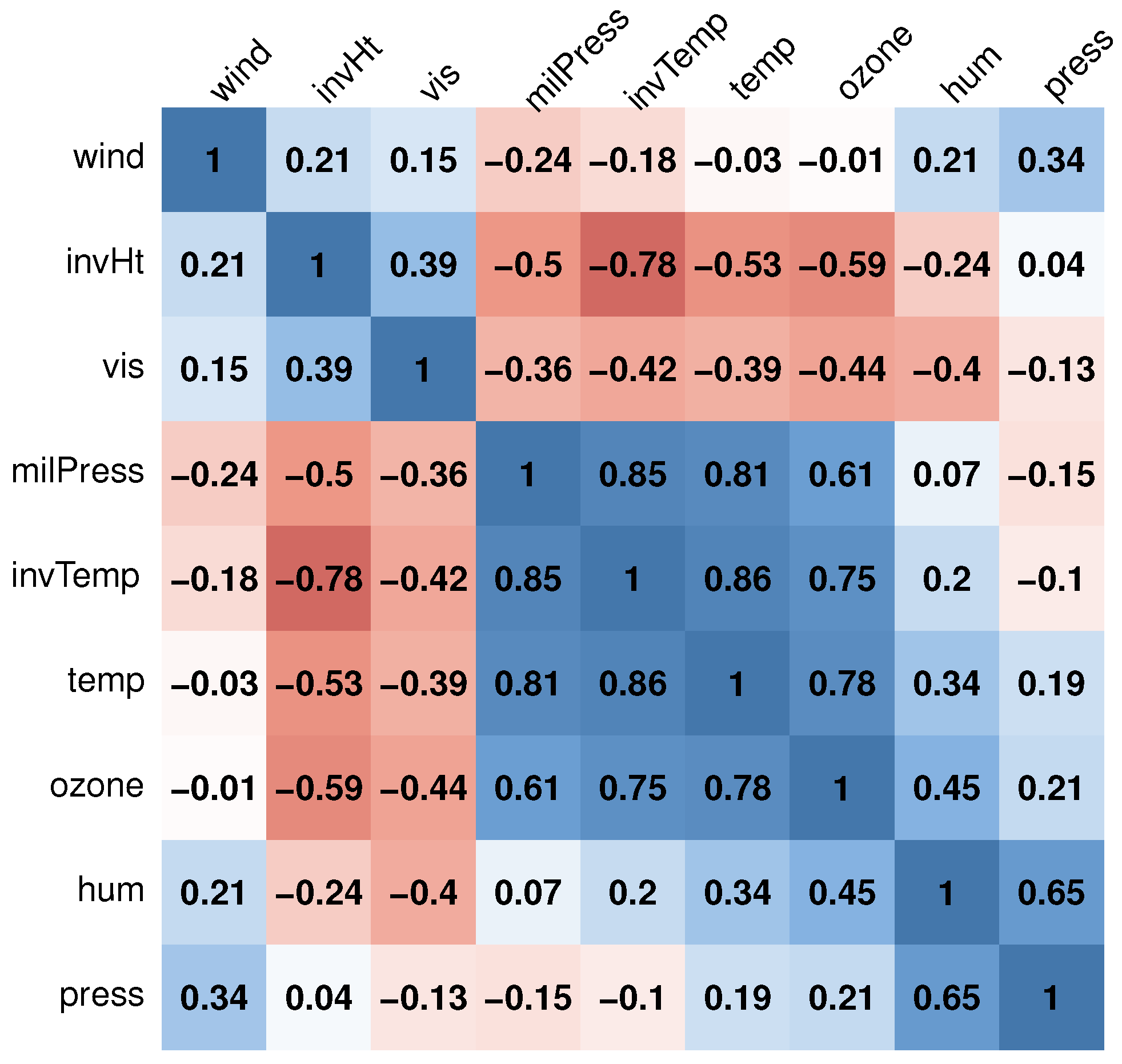
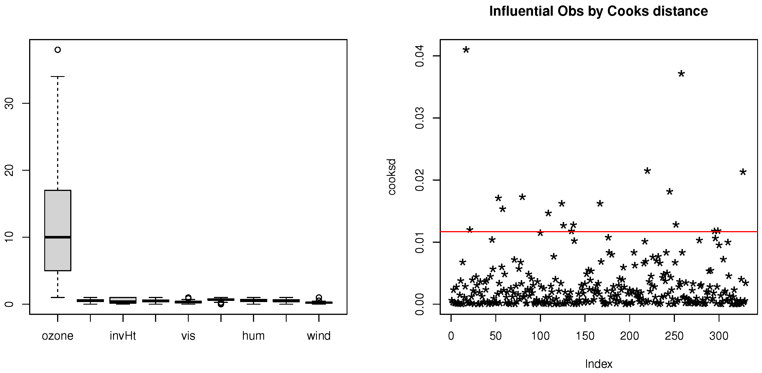
The paper’s structure is as follows: Section 2 provides a review of both classical and robust Lasso-type techniques. Section 3 introduces the diagnostic-Lasso estimator. Regression diagnostic measures are presented and discussed in Section 4. Section 5 offers a comparison of the proposed method’s performance against existing approaches, while Section 6 presents an analysis of the Los Angeles ozone data as an illustrative example. Finally, a concluding remark is presented in Section 7.

2. The Lasso Technique

2.1. Classical Lasso Estimator

Consider the situation in which the observed data are realizations of ${\left\{(\mathbf{X},y_i)\right\}}_{i=1}^n$ with a p-dimensional vector of covariates $\mathbf{X}\in {\mathbb{R}}^p$ and univariate continuous response variables $y_i\in \mathbb{R}$, a basic regression model has the following form: $y_i={\mathbf{X}}_i^T\mathit{\beta }+{ϵ}_i$, where $\mathit{\beta }$ is the set of regression coefficients and ${ϵ}_i$ is the ith error component. Tibshirani [1] assumed that $\mathbf{X}$ was normalized such that the mean and variance of each ocvariate ${\mathbf{X}}_k,$$k=1,\dots ,p$, is equal to 0 and 1, respectively. Letting $\widehat{\mathit{\beta }}=({\beta }_1,\dots ,{\beta }_p)$, the classical-Lasso estimate $\widehat{\mathit{\beta }}$ is defined by

$${\widehat{\mathit{\beta }}}_{Lasso}=arg\underset{\mathit{\beta }}{min}\sum _{i=1}^n{(y_i-{\mathbf{X}}_i^T\mathit{\beta })}^2+{\lambda }_{Lasso}\sum _{j=1}^p\left|{\beta }_j\right|,$$

(1)

where ${\lambda }_{Lasso}>0$ is a Lasso tuning parameter. The following adaptive Lasso (adl-Lasso) criterion, which is a modified Lasso criterion, is proposed by Zou [3]:

$${\widehat{\mathit{\beta }}}_{adl-Lasso}=arg\underset{\mathit{\beta }}{min}\sum _{i=1}^n{(y_i-{\mathbf{X}}_i^T\mathit{\beta })}^2+{\lambda }_{adl}\sum _{j=1}^p{\widehat{w}}_j^{adl}\left|{\beta }_j\right|,$$

(2)

where ${\widehat{w}}_j^{adl}=({\widehat{w}}_1^{adl},\dots ,{\widehat{w}}_p^{adl})$ a is a known weights vector.

2.2. Robust Lasso Estimator

When there are outliers in the data, the standard least squares method $LS$ fails to generate accurate estimates. The Lasso, however, is not robust against outliers since it is a particular instance of the penalized loss function of the $LS$ that is susceptible to the $L_1$ penalty function [14].

In these situations, we need to build a Lasso estimation method that can be used in multicollinearity situations and works well enough when there are outliers. The following equation gives the LAD-Lasso regression method proposed by [4]; it combines the least absolute deviation (LAD) and the Lasso methods and is only resistant to outliers in the response variable, as shown by [14],

$${\widehat{\mathit{\beta }}}_{LAD-Lasso}=arg\underset{\mathit{\beta }}{min}\sum _{i=1}^n|y_i-{\mathbf{X}}_i^T\mathit{\beta }|+{\lambda }_{LAD-Lasso}\sum _{j=1}^p\left|{\beta }_j\right|.$$

(3)

Combining Huber’s criterion with the adl-Lasso penalty, Ref. [5] produced another estimator that is resilient to heavy-tailed errors or outliers in the response. The Huber-Lasso estimator is written as follows:

$${\widehat{\mathit{\beta }}}_{Huber-Lasso}=arg\underset{\mathit{\beta }}{min}\sum _{i=1}^n{\mathcal{H}}_M\left(\frac{y_i-{\mathbf{X}}_i^T\mathit{\beta }}{s}\right)+{\lambda }_{Huber-Lasso}\sum _{j=1}^p{\widehat{w}}_j^{adl}\left|{\beta }_j\right|,$$

(4)

where $s>0$ is a distribution scaling parameter and ${\mathcal{H}}_M(.)$ is Huber’s criterion as loss function as introduced in [15] for every positive real M. For each positive real M, the ${\mathcal{H}}_M\left(z\right)$ expression is as follows:

$${\mathcal{H}}_M\left(z\right)=\left\{\begin{array}{c}{z}^2,for\mid z\mid \le M,\hfill \\ 2M\mid z\mid -M^2,for\mid z\mid >M,\hfill \end{array}\right.$$

The Sparse-LTS estimator proposed by [6] combines a least-trimmed squares estimator with a $L_1$ penalty as follows:

$${\widehat{\mathit{\beta }}}_{sparse-LTS}=arg\underset{\mathit{\beta }}{min}\sum _{i=1}^h{\left({\mathbf{r}}^2\left(\mathit{\beta }\right)\right)}_{i:n}+\lambda \sum _{j=1}^p\left|{\beta }_j\right|,$$

(5)

where ${\left({\mathbf{r}}^2\left(\mathit{\beta }\right)\right)}_{1:n}\le \dots \le {\left({\mathbf{r}}^2\left(\mathit{\beta }\right)\right)}_{n:n}$ are the order statistics of the squared residuals and $h\le n$ and ${\mathbf{r}}^2\left(\mathit{\beta }\right)={(r_1^2,\dots ,r_n^2)}^T$ denote the vector of squared with $r_i^2={(y_i-{\mathbf{X}}_i^T\mathit{\beta })}^2$. Ref. [6] showed in a simulation study that the Sparse-LTS can be robust against contamination in both the response and predictor variables. Ref. [7] proposed the MM-Lasso estimator, which combines MM-estimators with an adaptive $L_1$ penalty, and obtained lower bounds on the breakdown points of the MM-Lasso and adaptive MM-Lasso estimators. The MM-Lasso estimator is given as follows:

$${\widehat{\mathit{\beta }}}_{MM-Lasso}=arg\underset{\mathit{\beta }}{min}\sum _{i=1}^n{\rho }_1\left(\frac{r_i\left(\mathit{\beta }\right)}{s_n\left(\mathbf{r}\left({\widehat{\mathit{\beta }}}_0\right)\right)}\right)+\lambda \sum _{j=1}^p{\widehat{w}}_j^{adl}\left|{\beta }_j\right|,$$

(6)

where ${\rho }_1\le {\mathcal{H}}_M$, $r_i\left(\mathit{\beta }\right)=y_i-{\mathbf{X}}_i^T\mathit{\beta }$, ${\widehat{\mathit{\beta }}}_0$ is an initial consistent and high breakdown point estimate of $\mathit{\beta }$, $\mathbf{r}\left({\widehat{\mathit{\beta }}}_0\right)=y_i-{\mathbf{X}}_i^T{\widehat{\mathit{\beta }}}_0$, and $s_n\left(\mathbf{r}\left({\widehat{\mathit{\beta }}}_0\right)\right)$ is the M-estimate of the ${\widehat{\mathit{\beta }}}_0$ residuals’ scale.

3. Diagnostic-Lasso Estimator (D-Lasso)

This section proposes a new Lasso estimator based on the regression diagnostic method.

3.1. D-Lasso Estimator Formulation

A general idea to compute D-Lasso attempts first to create a clean, outlier-free subset of data. Let R represent the collection of observational indexes in the outlier-free subset, $y_{iR}$ and ${\mathbf{X}}_{iR}$ are observation subsets indexed by R, and ${\widehat{\mathit{\beta }}}_R$ are estimated regression coefficients obtained by fitting the model to the set R.

And let $SS{E}_R={\sum }_{i=1}^n{\left(y_{iR}-{\mathbf{X}}_{iR}^T{\mathit{\beta }}_R\right)}^2$ be the corresponding sum of squares residual that finds the estimates corresponding to the clean samples having the smallest sum of squares of residuals. As such, as expected, the breakdown point is 50%. When the number of collection of observational indexes in the outlier-free subset in R equal to n then ${\widehat{\mathit{\beta }}}_R=\widehat{\mathit{\beta }}$. This study suggests using $SS{E}_R$ in Lasso regression by replacing the value of ${\sum }_{i=1}^n{\left(y_i-{\mathbf{X}}_i^T\mathit{\beta }\right)}^2$ in Equation (1) by $SS{E}_R$. Thus, the D-Lasso can be expressed as follows:

$${\widehat{\mathit{\beta }}}_{D-Lasso}=argminSS{E}_R+{\lambda }_{D-Lasso}\sum _{j=1}^p\left|{\beta }_j\right|,$$

(7)

3.2. Breakdown Point

The replacement finite-sample breakdown point is the most commonly used measure of an estimator’s robustness.

3.2.1. Definition

Rousseeuw and Yohai [16,17] introduced the breakdown point of an estimator, which is defined as the minimum fraction of outliers that may take the estimator beyond any bound. In other words, the breakdown point of an estimate $\widehat{\mathit{\beta }}$ shows the effects of replacing several data values by outliers. The breakdown point for the regression estimator $\widehat{\mathit{\beta }}$ of the sample $\mathbf{Z}=(\mathbf{X},\mathbf{y})$ is defined as

$${\epsilon }^{*}(\widehat{\mathit{\beta }};\tilde{\mathbf{Z}})=min\left\{\frac{m}{n}:\underset{\tilde{\mathbf{Z}}}{sup}{\parallel \widehat{\mathit{\beta }}\left(\tilde{\mathbf{Z}}\right)\parallel }_2=\infty \right\},$$

where $\tilde{\mathbf{Z}}$ are contaminated data obtained from $\mathbf{Z}$ by replacing m of the original n data by outliers.

3.2.2. Breakdown Point of D-Lasso Estimator

The D-Lasso Estimator’s breakdown point for subsets of size $R\le n$ is provided by

$${\epsilon }^{*}({\widehat{\mathit{\beta }}}_R;Z_R)=\frac{(n-n_R+1)}{n}.$$

(8)

This study suggests taking a value of $n_R$ equal to a fraction $\alpha$ of the sample size, with $\alpha =0.75$, such that the final estimate is based on a sufficiently greater number of observations. This ensures a high enough statistical efficiency. The breakdown point that results from this is around $(1-\alpha )100\%=25\%$ (see [18]). Notice that the breakdown point is independent of the p dimension. Breakdown point is assured even if the number of predictor variables is greater than the sample size. Applying Equation (8) to the classical Lasso, which has ($n-n_R=0$), yields a finite sample breakdown point of ${\epsilon }^{*}({\widehat{\mathit{\beta }}}_{Lasso};Z)=\frac{1}{n}$ However, classical-Lasso is very sensitive to the presence of one outlier.

4. Regression Diagnostic Measures

4.1. Influential Observations in Regression

In this section, we introduce a different way of finding the clean subset R. A large body of literature is now available [10,11,12,13] for the identification of influential observations in linear regression. The Cook’s distance [19] and the differential of fits (DFFITS) [20] are two of the many influence measure that are currently accessible. The ith Cook’s distance is defined by [13] as:

$$C{D}_i=\frac{{({\widehat{\mathit{\beta }}}^{(-i)}-\widehat{\mathit{\beta }})}^T{\left({\mathbf{X}}^T\mathbf{X}\right)}^{-1}({\widehat{\mathit{\beta }}}^{(-i)}-\widehat{\mathit{\beta }})}{p{\widehat{\sigma }}^2},i=1,\dots ,n,$$

(9)

where ${\widehat{\mathit{\beta }}}^{(-i)}$ is the estimated parameter of $\mathit{\beta }$ with the ith observation deleted. The suggested cutoff point is $4/n$. Equation (9) can be expressed as:

$$C{D}_i\approx \frac{1}{p+1}{r}_{si}^2\left(\frac{h_{ii}}{1-h_{ii}}\right),$$

(10)

where $r_{si}$ is the ith standardized Pearson residual defined as:

$$r_{si}=\frac{y_i-{\mathbf{X}}_i^T{\widehat{\mathit{\beta }}}^{(-i)}}{\sqrt{{\widehat{\sigma }}_i^2(1-h_{ii}})},i=1,\dots ,n,$$

(11)

where $h_{ii}$ is the ith leverage value, which is in fact the ith diagonal element of the Hat matrix $H=\mathbf{X}{\left({\mathbf{X}}^T\mathbf{X}\right)}^{-1}{\mathbf{X}}^T$ and ${\widehat{\sigma }}_i$ is an appropriate estimate of $\sigma$.

The $DFFITS$ was introduced in [20], which is defined as:

$$DFFIT{S}_i=\frac{{\widehat{y}}_i-{\widehat{y}}_i^{(-i)}}{{\widehat{\sigma }}^{(-i)}\sqrt{h_{ii}}},i=1,\dots ,n,$$

(12)

where ${\widehat{y}}_i^{(-i)}$ and ${\widehat{\sigma }}^{(-i)}$ are, respectively, the ith fitted response and the estimated standard error with the ith observation deleted. The relationship between $C{D}_i$ and DFFITS is given by

$$C{D}_i=\frac{{\widehat{\sigma }}^{(-i)}}{p{\widehat{\sigma }}^2}DFFIT{S}_i^2.$$

Many other influence measures are available in the literature [11,21].

4.2. Identification of Multiple Influential Observations

The diagnostic tools discussed so far are designed for the identification of a single influential observation and are ineffective when masking and/or swamping occur. Therefore, we need detection techniques that are free from these problems. Ref. [12] introduced a group-deleted version of the residuals and weights in regression. Assume that d observations among a set of n observations are deleted. Let us denote a set of cases ‘remaining’ in the analysis by R and a set of cases ‘deleted’ by D. Therefore, R contains $(n-d)$ cases after d cases are deleted. Without loss of generality, assume that these observations are the last d rows of $\mathbf{X}$, y, and ${\sigma }_i$ (variance–covariance matrix) so that

$$\left[\begin{array}{c}{\mathbf{X}}_{iR}\\ {\mathbf{X}}_{iD}\end{array}\right],\left[\begin{array}{c}{y}_{iR}\\ y_{iD}\end{array}\right],\left[\begin{array}{cc}{\sigma }_R& 0\\ 0& {\sigma }_D\end{array}\right].$$

The generalized DFFITS (GDFFITS) is used [12] for the entire data set, defined as:

$$GDFFIT{S}_i=\left\{\begin{array}{cc}\frac{{\widehat{y}}_i^{(-D)}-{\widehat{y}}_i^{(-D-i)}}{{\widehat{\sigma }}^{(-D-i)}\sqrt{h_{ii}^{(-D)}}},& \mathrm{for}i\in R,\\ \frac{{\widehat{y}}_i^{(-D+i)}-{\widehat{y}}_i^{(-D)}}{{\widehat{\sigma }}^{(-D)}\sqrt{h_{ii}^{(-D+i)}}},& \mathrm{for}i\in K,\end{array}\right.$$

(13)

where ${\widehat{y}}_i^{(-D)}$ is the fitted response when a set of data indexed by D is omitted and

$$h_{ii}^{(-D+i)}={\mathbf{X}}^T{({\mathbf{X}}_R^T{\mathbf{X}}_R+\mathbf{X}{\mathbf{X}}^T)}^{-1}\mathbf{X}=\frac{h_{ii}^{(-D)}}{1-h_{ii}^{(-D)}},$$

where $h_{ii}^{(-D)}={\mathbf{X}}^T\left({\mathbf{X}}_R^T{\mathbf{X}}_R\right)\mathbf{X}$. The author considered observations as influential if $\left|GDFFIT{S}_i\right|$ $\ge 3\sqrt{p/(n-d)}$.

4.3. Tuning D-LASSO Parameter Estimation

Robust 5-fold cross validation was used to select the ${\lambda }_{D-Lasso}$ penalization parameter from a collection of possibilities, with a $\tau$-scale of the residuals serving as the objective function. The $\tau$-scale was introduced by [22] to estimate the largeness of the residuals in a regression model in a robust and effective manner.

To find a set of candidate values for $\lambda$, we selected 30 equally spaced points between 0 and ${\lambda }_{max}$, where ${\lambda }_{max}$ is about the smallest $\lambda$ for which all the coefficients of ${\widehat{\mathit{\beta }}}_{D-Lasso}\ne 0$ except the intercept.

To estimate ${\lambda }_{max}$, we first used bivariate winsorization [23] to robustly estimate the maximal correlation between $y_i$ and ${\mathbf{X}}_i$. This estimate was used as an initial guess for ${\lambda }_{max}$, and then a binary search was used to improve it. If $p>n$, then 0 is excluded from the candidate set.

5. Simulation Study

In this part, a simulation study that compared the proposed D-Lasso estimator’s performance to those of some other Lasso estimators is described. There are six estimators in the study: (i) D-Lasso, (ii) MM-Lasso, (iii) Sparse-LTS, (iv) Huber-LTS, (v) LAD-Lasso, and (vi) classical Lasso. Consider three different simulation scenarios:

Simulation 1: In the first simulation, multiple linear regression is taken into account with a sample size of 50 (n = 50) and 25 variables (p = 25), where each variable is selected from a joint Gaussian marginal distribution with a correlation structure of $\rho$ = 0.5.

The true regression parameters $\mathit{\beta }$ are set to be $(\underset{5}{\underbrace{1,2,3,4,5,}}\underset{20}{\underbrace{0,0,\dots ,0}})$. The distribution of random errors e is generated from the following contamination model: $F\left(e\right)=\left[\right(1-\epsilon \left)N\right(0,1)+\epsilon H(0,2\left)\right]\times \sigma$ where $\epsilon$ is the contamination ratio, $\sigma$ is the signal to noise, which is chosen to be 3, $N(0,1)$ is the standard normal distribution, and H is the Cauchy distribution to create a heavy-tailed distribution. The response variables are then calculated as follows:

$$y_{(50\times 1)}={\mathbf{X}}_{(50\times 25)}\times {(\underset{5}{\underbrace{1,2,3,4,5,}}\underset{20}{\underbrace{0,0,\dots ,0}})}^T+F{\left(e\right)}_{(50\times 1)}.$$

The percentage of zero coefficients (Z.coef) equals 80%, and the percentage of non-zero coefficients (N.Z coef.) equals 20%.

Simulation 2: The second simulation process is similar to the first, except that the p and n values are different (p = 50, n = 150), and the response variables are calculated as follows:

$$y_{(150\times 1)}={\mathbf{X}}_{(150\times 50)}\times {(\underset{5}{\underbrace{1,0,0,0,5,}}\underset{5}{\underbrace{0,1,0,0,5,}}\underset{5}{\underbrace{0,1,0,0,0,}}\underset{35}{\underbrace{0,0,\dots ,0}})}^T+F{\left(e\right)}_{(150\times 1)}$$

The percentage of true zero coefficients (Z.coef) equals 90% and the percentage of true non-zero coefficients (N.Z.coef) equals 10%.

Simulation 3: The third simulation is similar to the second, but n is increased to 500 and $\mathit{\beta }$=$(\underset{6}{\underbrace{1,0,0,0,5,0,}}\underset{5}{\underbrace{0,0,2,0,0,}}\underset{6}{\underbrace{1,0,0,0,0,5,}}\underset{33}{\underbrace{0,0,\dots ,0}}).$ The response variables are then calculated as follows:

$$y_{(500\times 1)}={\mathbf{X}}_{(500\times 50)}\times {\left(\mathit{\beta }\right)}^T+F{\left(e\right)}_{(500\times 1)}.$$

The percentage of true zero coefficients (Z.coef) equals 90% and the percentage of true non-zero coefficients (N.Z.coef) equals 10%.

The following data are looked at to see how well the approaches stand up to outliers and leverage points: (a) uncontaminated data; (b) vertical contamination (outliers on the response variables); (c) bad leverage points (outliers on the covariates).

The response variables and covariates are contaminated by certain ratios ($\epsilon$ = 0.05, 0.10, 0.15, and 0.20) of vertical and high leverage points; these are created by randomly replacing some original observations with large values equal to 15 [24].

The simulations were performed in statistical software R. D-Lasso, MM-Lasso, Sparse-LTS, Huber-Lasso, LAD-Lasso, and classical Lasso. Using the $GDFFITS$ measure suggested by [12], D-Lasso was assessed in order to determine which observations were influential, and ${\lambda }_{D-Lasso}$ was chosen as described in Section 4.3. For MM-Lasso we used the functions available in the github repository https://github.com/esmucler/mmlasso (accesses on 25 October 2017) [7].

The estimator was calculated using the sparseLTS() function from the robustHD package in R, and ${\lambda }_{Sparse-LTS}$ was chosen using a $BIC$ criterion as advocated by references [6]. Huber-Lasso used the package $MTE$ and the LAD-Lasso estimator was calculated using the package $flare$. The Lasso estimator was calculated using the lars() function from the lars package ([25]), where ${\lambda }_{Lasso}$ was chosen based on 5-fold cross-validation. ${\lambda }_{LAD-Lasso}$, and ${\lambda }_{Huber-Lasso}$, ${\lambda }_{MM-Lasso}$ were chosen by applying the classical $BIC$.

In each simulation run, there were 1000 replications. Four criteria are considered to evaluate the performances of the six methods, namely: (1) the percentage of zero coefficients (Z.coef), (2) the percentage of non-zero coefficients (N.Z.coef), (3) the average of mean squares of errors ($\overline{mse}$), and (4) the median of the mean squares of errors Med(mse). A good method for Simulation 1 is the one that possesses the percentage of Z.coef closed to 80% and the percentage of N.Z.coef closed to 20%. However, a good method for Simulations 2 and 3 is the one that possesses the percentage of Z.coef and N.Z.coef reasonably close to 90% and 10%, respectively, with a good method having the least ($\overline{mse}$) and Med(mse) values.

Several interesting points appear from the results of

Table 1. The results of three scenarios of simulation study for uncontaminated data.

	Lasso Estimators	Z.cof	N.Z.cof	$\overline{\mathit{m}\mathit{s}\mathit{e}}$	Med(mse)
Simulation 1	D-Lasso	77.6%	22.4%	45.1	77
	MM-Lasso	80.6%	19.4%	79.4	102.6
	Sparse-LTS	78.6%	21.4%	74	128.2
	Huber-LTS	82.1%	17.9%	83.6	119.0
	LAD-Lasso	76.2%	23.8%	88.2	81.3
	classical Lasso	80%	20%	26.9	22.1
Simulation 2	D-Lasso	90.6%	9.4%	25.1	17
	MM-Lasso	85.6%	14.4%	69.4	102.3
	Sparse-LTS	85.6%	14.4%	74	128.2
	Huber-LTS	90.1%	9.9%	91.6	61.0
	LAD-Lasso	92.2%	7.8%	98.9	91.8
	classical Lasso	89.9%	10.1%	16.9	12.1
Simulation 3	D-Lasso	91.9%	8.1%	25.1	17
	MM-Lasso	88.9%	11.1%	56	122.3
	Sparse-LTS	87.8%	12.2%	74	138.2
	Huber-LTS	90%	10%	96	106.0
	LAD-Lasso	92.1%	7.9%	59	98.8
	classical Lasso	90.2%	9.8%	6.6	2.1

,

Table 2. The results of three scenarios of simulation study for data with $\epsilon$ of vertical contamination.

		Lasso Estimators	Z.cof	N.Z.cof	$\overline{\mathit{m}\mathit{s}\mathit{e}}$	Med(mse)
$\epsilon =0.05$	Simulation 1	D-Lasso	81%	19%	3.8	3.1
		MM-Lasso	80.4%	19.6%	97	226
		Sparse-LTS	78%	22%	47	122
		Huber-LTS	82%	18%	68	111
		LAD-Lasso	76%	24%	84	85
		classical Lasso	44%	56%	87.3	308.4
	Simulation 2	D-Lasso	89%	11%	10.4	2.06
		MM-Lasso	85%	15%	96	123
		Sparse-LTS	85%	15%	76	121
		Huber-LTS	90%	10%	20	18
		LAD-Lasso	92%	8%	99	98
		classical Lasso	78%	22%	143.9	348.2
	Simulation 3	D-Lasso	88.8%	12.2%	15.5	4.7
		MM-Lasso	88%	12%	65	133
		Sparse-LTS	87%	13%	77	121
		Huber-LTS	90%	10%	98	102
		LAD-Lasso	92%	8%	98	102
		classical Lasso	75%	25%	168.1	374.2
$\epsilon =0.10$	Simulation 1	D-Lasso	85%	15%	6.6	5.5
		MM-Lasso	80.6%	19.4%	79.5	106
		Sparse-LTS	78.6%	21.4%	78	123
		Huber-LTS	82.2%	17.8%	86	196
		LAD-Lasso	76.2%	23.8%	88	84
		classical Lasso	41%	59%	167.5	321.3
	Simulation 2	D-Lasso	90%	10%	15.4	8.8
		MM-Lasso	85.6%	14.4%	69	101
		Sparse-LTS	85.6%	14.4%	78	123
		Huber-LTS	90.1%	9.9%	16	65
		LAD-Lasso	92.2%	7.8%	98.9	91.8
		classical Lasso	68%	32%	184.9	384.2
	Simulation 3	D-Lasso	90%	10%	40.9	10.9
		MM-Lasso	99.9%	11.1%	67	130
		Sparse-LTS	78.8%	12.2%	77	121
		Huber-LTS	90%	10%	97	97
		LAD-Lasso	92.1%	7.9%	93	87
		classical Lasso	65%	35%	105	482.4
$\epsilon =0.15$	Simulation 1	D-Lasso	83%	17%	6.7	6.0
		MM-Lasso	76%	24%	88	83
		Sparse-LTS	82%	18%	83	118
		Huber-LTS	78%	22%	76	113
		LAD-Lasso	80%	20%	74	101
		classical Lasso	38%	62%	349.6	323.1
	Simulation 2	D-Lasso	90%	10%	14.6	7.1
		MM-Lasso	92%	8%	91	98
		Sparse-LTS	90%	10%	19	14
		Huber-LTS	85%	15%	78	128
		LAD-Lasso	85%	15%	96	103
		classical Lasso	60%	40%	287.2	544.1
	Simulation 3	D-Lasso	90%	10%	34.8	14.7
		MM-Lasso	92%	8%	98	98
		Sparse-LTS	90%	10%	93	121
		Huber-LTS	87%	13%	78	134
		LAD-Lasso	88%	12%	69	131
		classical Lasso	57%	43%	374.6	448.0
$\epsilon =0.20$	Simulation 1	D-Lasso	81%	19%	7.7	6.8
		MM-Lasso	80%	20%	99	129
		Sparse-LTS	78.6%	21.4%	94	103
		Huber-LTS	82.1%	17.9%	86	98
		LAD-Lasso	76.2%	23.8%	89	98
		classical Lasso	36%	65%	246.9	562.6
	Simulation 2	D-Lasso	90%	10%	48.5	17.7
		MM-Lasso	85.6%	14.4%	69%	132
		Sparse-LTS	85.6%	14.4%	74	114
		Huber-LTS	90.1%	9.9%	19	23
		LAD-Lasso	92.2%	7.8%	91	98
		classical Lasso	58%	42%	316.8	471.5
	Simulation 3	D-Lasso	90%	10%	25.0	10.8
		MM-Lasso	88.9%	11.1%	98	131
		Sparse-LTS	87.8%	12.2%	89	89
		Huber-LTS	90%	10%	99	109
		LAD-Lasso	92.1%	7.9%	98	99
		classical Lasso	55%	45%	523.1	380.2

and

Table 3. The results of three scenarios of simulation study for data with $\epsilon$ of leverage points contamination.

		Lasso Estimators	Z.cof	N.Z.cof	$\overline{\mathit{m}\mathit{s}\mathit{e}}$	Med(mse)
$\epsilon =0.05$	Simulation 1	D-Lasso	80%	20%	4.9	4.2
		MM-Lasso	81%	19%	6.2	6.4
		Sparse-LTS	44%	56%	178	318
		Huber-LTS	40%	60%	176	318
		LAD-Lasso	16%	84%	138	308
		classical Lasso	45%	55%	88.4	219.5
	Simulation 2	D-Lasso	89%	11%	11.5	3.2
		MM-Lasso	88%	12%	12.7	5.4
		Sparse-LTS	78%	22%	143	318
		Huber-LTS	75%	25%	114	287
		LAD-Lasso	0%	100%	104	262
		classical Lasso	79%	21%	154.1	359.3
	Simulation 3	D-Lasso	90%	10%	16.6	5.8
		MM-Lasso	89%	11%	18.8	7.9
		Sparse-LTS	78%	22%	168	374
		Huber-LTS	77%	23%	155	490
		LAD-Lasso	0%	100%	155	474
		classical Lasso	76%	24%	179.2	385.3
$\epsilon =0.10$	Simulation 1	D-Lasso	81%	18	7.7	6.5
		MM-Lasso	80%	20%	9.1	8.7
		Sparse-LTS	44%	56%	457	332
		Huber-LTS	43%	57%	309	213
		LAD-Lasso	15%	85%	168	554
		classical Lasso	40%	58%	178.6	132.4
	Simulation 2	D-Lasso	90%	10%	16.5	9.9
		MM-Lasso	89%	11%	18.7	11.1
		Sparse-LTS	78%	22%	184.9	384
		Huber-LTS	77%	23%	545	461
		LAD-Lasso	0%	100%	554	888
		classical Lasso	69%	31%	295.1	495.3
	Simulation 3	D-Lasso	90%	10%	41.1	11.1
		MM-Lasso	89%	11%	62.3	22.3
		Sparse-LTS	78%	22%	310	428
		Huber-LTS	78%	22%	247	411
		LAD-Lasso	0%	100%	409	392
		classical Lasso	66%	34%	216	395.5
$\epsilon =0.15$	Simulation 1	D-Lasso	80%	20%	7.8	7.0
		MM-Lasso	89%	11%	9.1	9.2
		Sparse-LTS	45%	55%	334	321
		Huber-LTS	48%	52%	281	322
		LAD-Lasso	17%	83%	672	602
		classical Lasso	39%	61%	351.7	234.2
	Simulation 2	D-Lasso	90%	10%	15.6	8.2
		MM-Lasso	90%	10%	17.8	10.4
		Sparse-LTS	78%	22%	287	144
		Huber-LTS	79%	21%	178	772
		LAD-Lasso	0%	100%	156	716
		classical Lasso	61%	39%	298.3	155.2
	Simulation 3	D-Lasso	90%	10%	45.9	15.8
		MM-Lasso	88%	12%	67.2	27.1
		Sparse-LTS	78%	22%	372	281
		Huber-LTS	76%	24%	365	482
		LAD-Lasso	0%	100%	348	274
		classical Lasso	58%	42%	385.7	159.1
$\epsilon =0.20$	Simulation 1	D-Lasso	80%	20%	8.8	7.9
		MM-Lasso	79%	21%	10.1	9.1
		Sparse-LTS	44%	56%	246	262
		Huber-LTS	52%	48%	225	251
		LAD-Lasso	19%	81%	775	687
		classical Lasso	37%	64%	257.1	273.7
	Simulation 2	D-Lasso	90%	10%	59.4	28.8
		MM-Lasso	89%	11%	71.6	41.1
		Sparse-LTS	78%	22%	516	517
		Huber-LTS	81%	19%	205	207
		LAD-Lasso	1%	99%	485	377
		classical Lasso	59%	41%	327.9	182.6
	Simulation 3	D-Lasso	90%	10%	36.0	11.9
		MM-Lasso	89%	11%	58.2	22.3
		Sparse-LTS	41%	59%	311	280
		Huber-LTS	55%	45%	299	249
		LAD-Lasso	0%	100%	250	208
		classical Lasso	54%	44%	534.2	191.3

.

The results clearly show the merit of D-Lasso. It can be observed from Table 1, Table 2 and Table 3 that the D-Lasso has the smallest values of $\overline{mse}$ and Med(mse) compared to the other methods.

In the case of no contamination, Table 1 shows that both classical and D-Lasso methods perform well in model selection ability. For example, in the scenario of Simulation 1, the classical Lasso successfully selected 80% of Z.coef and 20% N.Z.coef, followed by D-Lasso, which selected 77.6% and 22.4% for Z.coef and N.Z.coef, respectively.

However, the performance of other robust lasso methods is good, but it has a larger $\overline{mse}$ and Med(mse) than the other two methods. Furthermore, none of the methods suffer from false selection variables.

In the case of vertical outliers and leverage points, the classical Lasso is clearly influenced by the outliers, as reflected in the much higher $\overline{mse}$ and Med(mse). Furthermore, it tended to select more variables in the final model (overfitting) when the percentage of contamination increased to 20%.

On the other hand, in the case of vertical outliers, the robust Lasso methods (MM-Lasso, Sparse, Huber-Lasso, and LAD-Lasso) clearly maintain their excellent behavior. Sparse-LTS has a considerable tendency toward false selection when the percentage of contamination increases to 20%. Table 2 shows that the robust Lasso methods (Sparse, Huber-Lasso, and LAD-Lasso) were affected by the presence of leverage points in the data. The effect was worse with a higher percentage of bad leverage points in the data.

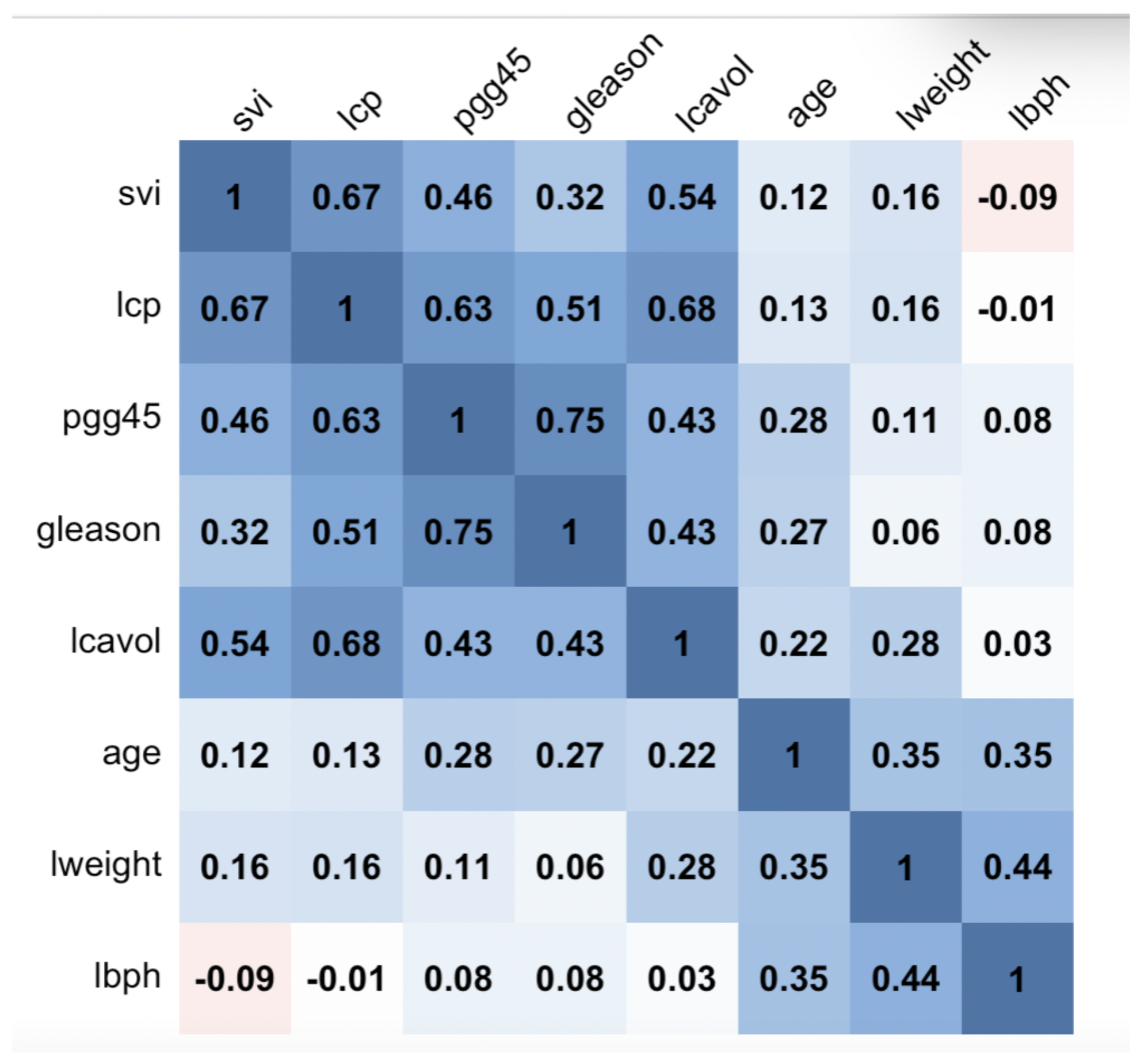
The results of D-Lasso and MM-Lasso are consistent for all percentages of contamination, but MM-Lasso has a larger $\overline{mse}$ than D-Lasso, which indicates that the performance of D-Lasso is more efficient than the other methods. For further illustrative purposes, the forthcoming section analyzes some real data sets.

6. Application to Real Data

6.1. Ozone Data

To assess the performance of D-Lasso in comparison with other Lasso methods, we analyzed the Los Angeles ozone pollution data, as originally studied by [26], which is available in the R package ‘cosso’. The Ozone dataset comprises 330 observations, each representing daily measurements of nine meteorological variables. The ozone reading serves as the predicted variable, while the remaining eight covariates are temperature (temp), inversion base height (invHt), pressure (press), visibility (vis), millibar pressure height (milPress), humidity (hum), inversion base temperature (invTemp), and wind speed (wind).

Figure 1 displays the correlation matrix of the meteorological variables, revealing significant correlations between the following pairs: (temp and invTemp), (invHt and invTemp), (milPress and invTemp), and (milPress and temp). Additionally, the Variance Inflation Factor ($VIF$), calculated as $VIF=\frac{1}{1-R_j^2}$, quantifies the increase in variance due to correlations among explanatory variables, where $R_j^2$ represents the unadjusted coefficient of determination for regressing the jth independent variable [27]. A commonly used default $VIF$ cutoff value is 5; only variables with a $VIF$ less than 5 are included in the model. If one or more variables in a regression exhibit high $VIF$ values, it indicates collinearity.

The $VIF$ values of the predictors for the Ozone data are provided in

Table 4. The $VIF$ for the covariates of the multiple regression model for Ozone data set.

Variable	Temp	invHt	Press	Vis	milPress	Hum	invTemp	Wind
$VIF$	8.626	4.319	2.658	1.459	5.372	2.271	18.037	1.283

. It is evident that invTemp has the highest $VIF$ value, followed by temp.

To identify potential outliers in the Ozone data, we used the function “outlier” in R, and we employed boxplots for the variables and evaluated Cook’s distance in a multiple regression model. Consequently, the Ozone dataset reveals the presence of one vertical outliers at row 38 and three leverage points, as illustrated in Figure 2.

We utilized the $GDFFITS$ measure to detect outliers in the proposed D-Lasso estimators, while applying other Lasso methods for comparative purposes. We also calculated the Root Mean Squared Error ($RMSE$) and R-squared values for these methods.

Table 5. The six Lasso estimators methods for the Ozone data set.

Variables	Classical-Lasso	LAD-Lasso	Huber-Lasso	Sparce-LTS	MM-Lasso	D-Lasso
intercept	−1.6758	−1.8422	−0.0124	1.8786	3.3786	−0.9643
temp	17.9711	18.5883	19.8520	16.8129	15.2957	18.3841
invHt	−2.9138	−3.2466	−4.3513	−2.8686	−3.4073	0
press	0	0	0	0	0	0
vis	−1.5399	0	−1.4379	0	0	0
milPress	0	0	0	0	0	0
hum	5.4193	5.8341	5.0834	2.5183	1.7916	3.0894
invTemp	5.5373	5.2498	0	0	0	0
wind	0	0	0	0	0	0
$R^2$	0.5623	0.6198	0.7070	0.7594	0.7988	0.9220
$RMSE$	5.9123	5.1248	4.5277	4.4334	4.4578	3.7297
Z.coef	3	3	5	5	5	6
NZ.coef	6	6	4	4	4	3

presents the results of the various Lasso methods. Notably, classical Lasso and LAD-Lasso selected six non-zero coefficients, albeit with higher $RMSE$ values. In contrast, Huber-Lasso, Sparse-LTS, and MM-Lasso selected four non-zero coefficients. D-Lasso, on the other hand, selects three non-zero coefficients (intercept, temp, and hum). The $RMSE$ values of D-Lasso are smaller than those of Huber-Lasso, Sparse-LTS, and MM-Lasso, signifying the greater reliability of D-Lasso for this dataset.

Furthermore, Table 5 demonstrates that across different Lasso criteria, the R-squared values of D-Lasso, Sparse-LTS, and MM-Lasso estimators are notably more acceptable than the R-squared values of other Lasso estimators.

6.2. Prostate Cancer Data

The Prostate cancer dataset encompasses 97 observations from male patients aged between 41 and 79 years. This dataset was originally sourced from a study conducted by [28] and is accessible through the R package ’genridge’. The response variable is the log(prostate specific antigen), denoted as Ipsa, while the explanatory variables include log(cancer volume) (lcavol), log(prostate weight) (lweight), age, log(benign prostatic hyperplasia amount) (lbph), seminal vesicle invasion (svi), log(capsular penetration) (lcp), Gleason score (gleason), percentage of Gleason scores 4 or 5 (pgg45), and log(prostate specific antigen) (lpsa).

Figure 3 presents the correlation matrix of these variables, highlighting significant correlations between the following pairs: (pgg45, gleason) and (lcp, lcavol). Furthermore, the Variance Inflation Factor ($VIF$) values for the predictors in the Prostate cancer data are provided in

Table 6. The $VIF$ for the covariates of the multiple regression model for Prostate cancer data set.

Variable	Lcavol	Lweight	Age	Lbph	svi	Lcp	Gleason	Pgg45
$VIF$	2.102	1.453	1.336	1.385	1.955	5.097	2.468	5.974

, with pgg45 exhibiting the highest $VIF$ value, followed by lcp.

To identify potential outliers in the Prostate cancer data, we used the function “outlier” in R, and we employed boxplots for the variables and assessed Cook’s distance in a multiple regression model. As illustrated in Figure 4, the Prostate cancer dataset contains two vertical outliers and five leverage points.

For the identification of outliers in the proposed D-Lasso estimators, we utilized the $GDFFITS$ measure, while other Lasso methods were applied for comparative analysis. We also calculated the Root Mean Squared Error ($RMSE$) and R-squared values for these methods.

Table 7. The six Lasso estimators methods for Prostate cancer data set.

Variables	Classical-Lasso	LAD-Lasso	Huber-Lasso	Sparce-LTS	MM-Lasso	D-Lasso
intercept	0.4339	0	0.3280	0.0677	2.4472	0.5809
lcavol	0.5113	0.5482	0.5131	0.5628	0.5568	0.3418
lweight	0.3292	0.4772	0.3531	0.4161	0	0.3388
age	0	−0.0228	0	0	−0.0138	−0.1239
lbph	0.0421	0.1604	0.0525	0.0139	0.1303	0.0767
svi	0.5436	0.7777	0.5571	0.5993	0.6551	0.6361
lcp	0	−0.0938	0	0	0	0
gleason	0	0.1826	0	0	0	0.0020
pgg45	0.0012	0	0.0016	0	0.0014	0
$R^2$	0.5623	0.3619	0.7070	0.7594	0.5921	0.8932
$RMSE$	6.912	3.1248	4.5277	2.4334	4.4578	1.7297
Z.coef	3	2	3	4	3	2
NZ.coef	6	7	6	5	6	7

presents the results of the different Lasso methods. Classical Lasso, Huber-Lasso, and MM-Lasso each select six non-zero coefficients, albeit with higher $RMSE$ values. In contrast, LAD-Lasso selects seven non-zero coefficients with an $RMSE$ of 3.1248, while Sparce-LTS selects five non-zero coefficients with an $RMSE$ of 2.4334.

D-Lasso, on the other hand, selects two zero coefficients (lcp and pgg45), and the $RMSE$ value of D-Lasso is smaller than that of other methods. Consequently, D-Lasso is considered more reliable for this dataset.

7. Conclusions

The classical Lasso technique is often utilized for creating regression models, but it can be influenced by the presence of vertical and high leverage points, leading to potentially misleading results. A robust version of the Lasso estimator is commonly derived by replacing the ordinary squared residuals ($LS$) function with a robust alternative.

This article aims to introduce robust Lasso methods that utilize regression diagnostic tools to detect suspected outliers and high leverage points. Subsequently, the D-Lasso is computed following diagnostic checks.

To assess the effectiveness of our newly proposed approaches, we conducted comparisons with the classical Lasso and existing robust Lasso methods based on LAD, Huber, Sparse-LTS, and MM estimators using both simulations and real datasets.

In this article, D-Lasso regression serves as the primary variable selection technique. Future endeavors may delve into exploring the asymptotic theoretical aspects and establishing the oracle properties of D-Lasso.

References

1. Tibshirani, R. Regression shrinkage and selection via the lasso. J. R. Stat. Soc. Ser. B (Methodol.) 1996, 58, 267–288. [Google Scholar] [CrossRef]
2. Fan, J.; Li, R. Variable selection via nonconcave penalized likelihood and its oracle properties. J. Am. Stat. Assoc. 2001, 96, 1348–1360. [Google Scholar] [CrossRef]
3. Zou, H. The adaptive lasso and its oracle properties. J. Am. Stat. Assoc. 2006, 101, 1418–1429. [Google Scholar] [CrossRef]
4. Wang, H.; Li, G.; Jiang, G. Robust regression shrinkage and consistent variable selection through the LAD-Lasso. J. Bus. Econ. Stat. 2007, 25, 347–355. [Google Scholar] [CrossRef]
5. Lambert-Lacroix, S.; Zwald, L. Robust regression through the Huber’s criterion and adaptive lasso penalty. Electron. J. Stat. 2011, 5, 1015–1053. [Google Scholar] [CrossRef]
6. Alfons, A.; Croux, C.; Gelper, S. Sparse least trimmed squares regression for analyzing high-dimensional large data sets. Ann. Appl. Stat. 2013, 7, 226–248. [Google Scholar] [CrossRef]
7. Smucler, E.; Yohai, V.J. Robust and sparse estimators for linear regression models. Comput. Stat. Data Anal. 2017, 111, 116–130. [Google Scholar] [CrossRef]
8. Simpson, L.; Combettes, P.L.; Müller, C.L. C-lasso—A Python package for constrained sparse and robust re-gression and classification. J. Open Source Softw. 2020, 6, 2844. [Google Scholar] [CrossRef]
9. Chang, L.; Welsh, A.H. Robust Multivariate Lasso Regression with Covariance Estimation. J. Comput. Graph. Stat. 2022, 32, 961–973. [Google Scholar] [CrossRef]
10. Atkinson, A.C.; Riani, M.; Riani, M. Robust Diagnostic Regression Analysis, 2nd ed.; Springer: New York, NY, USA, 2000. [Google Scholar]
11. Chatterjee, S.; Hadi, A.S. Regression Analysis by Example; John Wiley & Sons. Inc.: Hoboken, NJ, USA, 2006. [Google Scholar]
12. Rahmatullah Imon, A. Identifying multiple influential observations in linear regression. J. Appl. Stat. 2005, 32, 929–946. [Google Scholar] [CrossRef]
13. Ryan, T.P. Modern Regression Methods; John Wiley & Sons: Hoboken, NJ, USA, 2008; p. 655. [Google Scholar]
14. Alshqaq, S.S.A. Robust Variable Selection in Linear Regression Models. Doctoral Dissertation, Institut Sains Matematik, Fakulti Sains, Universiti Malaya, Kuala Lumpure, Malaysia, 2015. [Google Scholar]
15. Huber, P.J. Robust Statistics; Wiley: New York, NY, USA, 1981. [Google Scholar]
16. Maronna, R.A.; Martin, R.D.; Yohai, V.J. Robust Statistics: Theory and Methods; Wiley Series in Probability and Statistics; John Wiley & Sons: Hoboken, NJ, USA, 2006. [Google Scholar]
17. Rousseeuw, P.; Yohai, V. Robust regression by means of s-estimators. In Robust and Nonlinear Time Series Analysis; Springer: Berlin/Heidelberg, Germany, 1984; pp. 256–272. [Google Scholar]
18. Saleh, S.; Abuzaid, A.H. Alternative Robust Variable Selection Procedures in Multiple Regression. Stat. Inf. Comput. 2019, 7, 816–825. [Google Scholar] [CrossRef]
19. Cook, R.D. Detection of influential observation in linear regression. Technometrics 1977, 19, 15–18. [Google Scholar]
20. Belsley, D.A.; Kuh, E.; Welsch, R.E. Regression Diagnostics: Identifying Influential Data and Sources of Collinearity; John Wiley & Sons: Hoboken, NJ, USA, 2005. [Google Scholar]
21. Hadi, A.S. A new measure of overall potential influence in linear regression. Comput. Stat. Data Anal. 1992, 14, 1–27. [Google Scholar] [CrossRef]
22. Yohai, V.J.; Zamar, R.H. High breakdown-point estimates of regression by means of the minimization of an efficient scale. J. Am. Stat. Assoc. 1988, 83, 406–413. [Google Scholar] [CrossRef]
23. Khan, J.A.; Van Aelst, S.; Zamar, R.H. Robust linear model selection based on least angle regression. J. Am. Stat. Assoc. 2007, 102, 1289–1299. [Google Scholar] [CrossRef]
24. Uraibi, H.; Midi, H. Robust variable selection method based on huberized LARS-Lasso regression. Econ. Comput. Econ. Cybern. Stud. Res. 2020, 54, 145–160. [Google Scholar]
25. Hastie, T.; Efron, B. Lars: Least Angle Regression, Lasso and Forward Stagewise; R Package; Version 1.2. Available online: https://CRAN.R-project.org/package=lars (accessed on 15 November 2018).
26. Breiman, L.; Friedman, J. Estimating Optimal Transformations for Multiple Regression and Corre-lation. J. Am. Stat. Assoc. 1985, 80, 580–598. [Google Scholar] [CrossRef]
27. Fox, J. Regression Diagnostics: An Introduction; Sage Publications: New York, NY, USA, 2019. [Google Scholar]
28. Stamey, T.A.; Kabalin, J.N.; McNeal, J.E.; Johnstone, I.M.; Freiha, F.; Redwine, E.A.; Yang, N. Prostate specific antigen in the diagnosis and treatment of adenocarcinoma of the prostate. II. Radical prostatectomy treated patients. J. Urol. 1989, 141, 1076–1083. [Google Scholar] [CrossRef] [PubMed]
Figure 1. Correlation matrix of variables in the Ozone data set. The colors reflect sign of correlation, where red reveals negative correlation and blue reveals a positive correlation.
Symmetry 15 02155 g001
Figure 2. Boxplot of predictors (left) and Cook’s distance (an observations over red line have too much influence) (right) for Ozone data set.
Symmetry 15 02155 g002
Figure 3. Correlation matrix of variables in the Prostate cancer data set. The colors reflect sign of correlation, where red reveals negative correlation and blue reveals a positive correlation.
Symmetry 15 02155 g003
Figure 4. Boxplot of predictors (left) and Cook’s distance (an observations over red line have too much influence, and red numders show the row number of influence obevation in data) (right) for Prostate cancer data set.
Symmetry 15 02155 g004