Application of Diversity-Maintaining Adaptive Rafflesia Optimization Algorithm to Engineering Optimisation Problems

Abstract

The Diversity-Maintained Adaptive Rafflesia Optimization Algorithm represents an enhanced version of the original Rafflesia Optimization Algorithm. The latter draws inspiration from the unique characteristics displayed by the Rafflesia during its growth, simulating the entire lifecycle from blooming to seed dispersion. The incorporation of the Adaptive Weight Adjustment Strategy and the Diversity Maintenance Strategy assists the algorithm in averting premature convergence to local optima, subsequently bolstering its global search capabilities. When tested on the CEC2013 benchmark functions under a dimension of 30, the new algorithm was compared with ten optimization algorithms, including commonly used classical algorithms, such as PSO, DE, CSO, SCA, and the newly introduced ROA. Evaluation metrics included mean and variance, and the new algorithm outperformed on a majority of the test functions. Concurrently, the new algorithm was applied to six real-world engineering problems: tensile/compressive spring design, pressure vessel design, three-bar truss design, welded beam design, reducer design, and gear system design. In these comparative optimizations against other mainstream algorithms, the objective function’s mean value optimized by the new algorithm consistently surpassed that of other algorithms across all six engineering challenges. Such experimental outcomes validate the efficiency and reliability of the Diversity-Maintained Adaptive Rafflesia Optimization Algorithm in tackling optimization challenges. The Diversity- Maintained Adaptive Rafflesia Optimization Algorithm is capable of tuning the parameter values for the optimization of symmetry and asymmetry functions. As part of our future research endeavors, we aim to deploy this algorithm on an even broader array of diverse and distinct optimization problems, such as the arrangement of wireless sensor nodes, further solidifying its widespread applicability and efficacy.

1. Introduction

1.1. Meta-Heuristic Algorithms

In recent years, with the rapid development of intelligent optimization algorithms, numerous optimization problems have been addressed effectively. An optimization problem is characterized by the quest to find the best solution or parameter values that maximize or minimize an objective function within a vast array of solutions and parameters, subject to certain constraints. Meta-heuristic optimization algorithms are useful to solve both the optimization of symmetry functions and asymmetry functions with constrains. These problems encompass essential components such as the objective function, variables, and constraints. The domains covered by optimization problems are diverse, spanning areas such as engineering optimization, data mining, machine learning, wireless sensor deployment, resource scheduling, digital image processing, mechanical design, and path planning, among others. When confronted with these challenges, traditional optimization methods, such as Newton’s method, necessitate an exhaustive traversal of the entire search space, a process that is often time-consuming. In the context of specific complex optimization issues, due to the vastness of their search spaces, high complexity, and the presence of constraints and nonlinearities, pinpointing the optimal solutions becomes increasingly challenging. Hence, there is a pronounced emphasis on seeking high-performance, rapidly converging intelligent optimization algorithms to tackle these intricate problems.

Inspired by natural social laws and collective biological behaviors, researchers have begun to introduce a category of algorithms known as metaheuristic algorithms. Compared to traditional optimization algorithms, these metaheuristics exhibit superior robustness, explorative capacity, and adaptability. Some metaheuristic algorithms, originating as early as the 1970s and 1980s, have been proposed. For instance, the classic Genetic Algorithm and Simulated Annealing Algorithm were introduced, leveraging the simulation of natural biological evolution and the annealing process of solid materials to search spaces for optimal solutions. Empirical tests indicated that these algorithms achieved favorable outcomes in solving intricate problems.

With the continued evolution of scientific research, an increasing number of metaheuristic algorithms have been developed and studied. In 1995, for example, Storn and colleagues introduced the Differential Evolution Algorithm, rooted in swarm intelligence theory. Initially conceived for Chebyshev polynomial problems, it was subsequently found to be effective for other optimization problems. There are numerous algorithms based on swarm intelligence, such as Particle Swarm Optimization [1] (PSO), inspired by the flocking and clustering behaviors of birds during foraging. Owing to its simplicity and ease of implementation, PSO quickly garnered considerable attention. By simulating the behavior of ants in their unaided search for the shortest route between food and their nest, Ant Colony Optimization [2,3] (ACO) was proposed, primarily for shortest-path problems. Drawing inspiration from the behavioral traits and hunting strategies of cats, researchers introduced Cat Swarm Optimization [4] (CSO). By emulating the echolocation features and flight patterns of bats, researchers presented the Bat Algorithm [5,6] (BA). The Sine-Cosine Algorithm [7] (SCA), developed based on the continuity and periodicity of sine and cosine functions, simulates solution optimization and searching. In recent years, newer optimization algorithms have emerged, such as the Goose Optimization Algorithm [8] (GOA), which is founded on the behavior of geese during predation, particularly their exploratory behavior prior to spotting fish and their chasing behavior once fish are detected. The Artificial Fish Swarm Algorithm [9,10] (AFSA) was proposed, inspired by fish interactions during predation and predator avoidance. The Artificial Bee Colony Algorithm [11] (ABCA) emanates from bee foraging behaviors, replicating the bees’ information exchange and foraging strategies. Bamboo Forest Optimization [12] (BFGO) was inspired by the growth characteristics of bamboo, while the Rafflesia Optimization Algorithm [13] (ROA) and the Binary Rafflesia Optimization Algorithm were conceived based on the blooming and reproduction patterns of the Rafflesia flower. The Grey Wolf Optimizer [14,15] (GWO) mimics the societal behaviors of grey wolves, particularly in their hunting endeavors. Based on the migratory and foraging behaviors of whales, the Whale Optimization Algorithm [16,17] (WOA) was introduced to optimize solution spaces. Additionally, algorithms such as the Gaining–Sharing Knowledge-Based Algorithm [18] (GSK) have been introduced. Upon their introduction, these metaheuristic algorithms have been successfully deployed in path planning, engineering applications, and sensor placements, among other complex optimization challenges, consistently delivering commendable results.

With the continued advancements in intelligent optimization algorithms in recent years, numerous optimization strategies have been proposed by researchers and successfully applied to real-world optimization problems. However, no single algorithm has been identified that can universally address all optimization challenges. This observation aligns with the No Free Lunch Theorem. When confronted with a particular complex optimization problem, an algorithm might produce commendable outcomes post-optimization. Yet, the same algorithm may underperform when tasked with different challenges. This suggests that algorithms can often become trapped in local optima when applied in practical scenarios. To mitigate this issue, researchers have sought to refine existing algorithms and introduce enhanced ones, aiming to bolster their convergence capabilities. One such effort, the Butterfly Optimization Algorithm (BOA), was indeed grounded in the No Free Lunch Theorem.

To achieve superior convergence results, modifications were made to the Rafflesia Optimization Algorithm, incorporating adaptive weight adjustment strategies and diversity preservation techniques. This revamped algorithm, designed to avoid local optima entrapments and demonstrate augmented convergence capabilities, has been termed the Diversity-Maintained Adaptive Rafflesia Optimization Algorithm (AROA). Subsequently, the AROA’s performance was assessed and tested using the CEC2013 benchmark function set. It was compared with algorithms such as ROA, PSO, SCA, WOA, GSA [19], DE [20,21], CSO [22], BA, and BOA for problems with a dimensionality of 30. Comparative outcomes revealed that AROA exhibited superior convergence performance. Moreover, AROA was applied to engineering optimization problems to gauge its efficacy in practical applications. When juxtaposed with other algorithms in this context, AROA consistently delivered superior results.

1.2. Algorithmic Features or Principles

Meta-heuristic algorithms, such as Particle Swarm Optimization (PSO), Ant Colony Optimization (ACO), Cat Swarm Optimization (CSO), the Artificial Bee Colony Algorithm (ABCA), Artificial Fish Swarm Algorithm (AFSA), Grey Wolf Optimizer (GWO), Whale Optimization Algorithm (WOA), Bat Algorithm (BA), Sine-Cosine Algorithm (SCA), Gaining–Sharing Knowledge-Based Algorithm (GSK), and the Rafflesia Optimization Algorithm (ROA), are evolutionary or swarm intelligence algorithms designed to address optimization problems. The fundamental distinctions between them lie in their basic principles and characteristics.

A common trait amongst these algorithms is that they emulate behaviors observed in nature or mathematical principles to identify optimal solutions. For instance, PSO mimics the flocking behavior of birds, ACO simulates ant foraging, and CSO emulates hunting behavior of cats. These algorithms employ various strategies to guide their search processes, exploring the search space to eventually pinpoint either global optima or high-quality solutions.

However, these meta-heuristic algorithms have unique foundational principles and essential characteristics. For instance, in PSO, which imitates the flocking behavior of birds, particles adjust their velocities and positions based on personal and global best positions. ACO, drawing inspiration from ants searching for food, uses pheromones as guidance for the search process. CSO, emulating cat hunting and migration behaviors, introduces hunting and migration phases to enhance diversity. ABCA mirrors bee recruiting, foraging, and information-sharing behaviors, fostering inter-bee cooperation to pinpoint optimal solutions. AFSA emulates fish foraging and migration, encompassing both individual and collective behaviors. GWO replicates social behaviors within wolf packs, incorporating alpha leadership and followership. WOA imitates whale search and foraging, integrating linearly decreasing predation behaviors. BA emulates bat foraging and echolocation, using frequency and amplitude adjustments for exploration. SCA employs the mathematical principles of sine and cosine functions to generate novel solutions, while GSK, predicated on knowledge-sharing and acquisition mechanisms, optimizes solutions through individual cooperation.

Regarding application domains, certain algorithms, such as PSO, GWO, and ROA, are more suited for continuous optimization problems, whereas ACO and CSO are tailored for discrete optimization problems. Algorithms such as ABCA and AFSA can often be employed across diverse problem types, including both continuous and discrete optimization.

From an information dissemination perspective, ACO deploys pheromones to guide the search, with pheromone deposition and evaporation influencing path selection. ABCA and AFSA, despite also involving information dissemination, differ in their mechanisms: bees and fish collaborate and exchange information to locate optimal solutions.

In terms of update strategies, algorithms such as CSO, AFSA, and GWO introduce unique diversity maintenance strategies, such as hunting and migration behaviors and individual versus collective behaviors, to enhance search diversity. In summary, the critical distinguishing features among these meta-heuristic algorithms encompass their foundational principles, application domains, information dissemination mechanisms, diversity maintenance strategies, parameter tuning, and adaptiveness. The choice of the appropriate algorithm largely depends on the nature and specific requirements of the problem at hand.

The advantages of these algorithms over traditional optimization techniques lie in their ability to guide a search by simulating behaviors observed in nature or by leveraging mathematical principles, thereby enhancing their exploration capabilities for complex, multimodal problems. During the search process, they are able to maintain diversity and possess both global and local search capabilities. As a result, they are typically more adept at locating global optima or high-quality solutions. The choice of algorithm often hinges upon the specific nature of the problem and the configuration of algorithmic parameters. The flexibility and versatility of these algorithms render them potent tools for addressing a wide array of optimization challenges.

The remaining structure of this paper is organized as follows: Section 2 presents the preparatory work, introducing the original Rafflesia Optimisation Algorithm, the strategies employed for the improved algorithm, and the optimization domains and challenges addressed in this study. Section 3 delves into the specific improvement details of applying the adaptive weight adjustment strategy and diversity maintenance strategy to the Rafflesia Optimisation Algorithm. Section 4 conducts tests on the algorithm, presenting comparative test results and their analysis. Section 5 evaluates the algorithm’s performance in engineering application problems. Section 6 discusses the algorithm’s applicability and time complexity and also highlights the performance capabilities of some benchmark algorithms. The final section, Section 7, summarizes the main research contributions of this paper and offers perspectives on future research directions.

2. Related Works

This section predominantly delineates the specific algorithmic procedure of the original Rafflesia Optimization Algorithm. Additionally, two strategies employed to enhance the Rafflesia Optimization Algorithm are detailed: the adaptive weight adjustment strategy and the diversity maintenance strategy. The section concludes by identifying the optimization domains and challenges addressed in this paper and proposing the optimization processes tailored to these specific areas.

2.1. ROA

The inspiration for the Rafflesia Optimization Algorithm is derived from all the behavior of the Rafflesia flower, from its blooming onset to seed propagation. Drawing upon the characteristics exhibited during the Rafflesia’s growth process, this algorithm emulates certain distinctive features evident from its budding phase through to seed dispersion. Firstly, when the Rafflesia begins to bloom, it emits a scent to allure insects. Secondly, once insects are attracted by the fragrance released upon the Rafflesia’s blooming, they assist the flower in the pollination process. However, due to the Rafflesia’s unique floral chamber structure, certain insects can become trapped during pollination, ultimately leading to their demise. Thirdly, once the Rafflesia’s petals wither, it yields a fruit laden with a multitude of seeds. The seeds produced by the Rafflesia are dispersed in various ways for propagation in diverse locales. Owing to environmental constraints, only a minimal number of these seeds manage to endure. Taking into account these three distinctive traits of the Rafflesia, the algorithm has been segmented into three phases: the insect attraction phase, the insect consumption phase, and the seed dissemination phase. Furthermore, the algorithm regards the optimal solution as the insect positioned nearest to the Rafflesia.

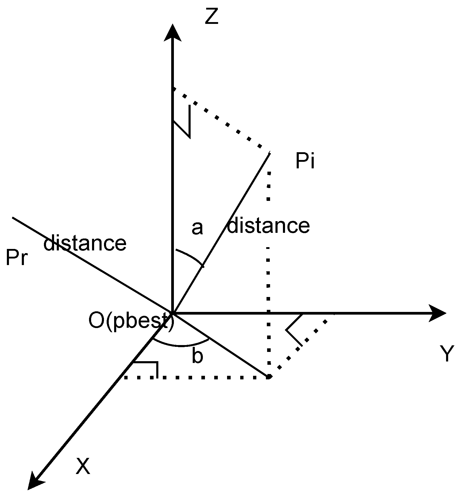
2.1.1. Attracting Insects Stage

In the initial phase, the ROA employs two strategies. The first strategy addresses the relationship between insects newly attracted by the Rafflesia and those not flying towards the Rafflesia. The second strategy is utilized to update the status of insects consistently heading towards the Rafflesia.

Due to the individuals in the population existing within a multi-dimensional space for which a suitable coordinate system has yet to be constructed in reality, an abstraction to a three-dimensional space is utilized for computational purposes for each dimension of the new individuals. The position of these new individuals is computed with reference to a mathematical model exemplified in Figure 1. This three-dimensional space is composed of the X, Y, and Z axes, where Y and Z represent two arbitrary dimensions that are perpendicular to the X axis within the multi-dimensional space.

In Strategy I, individuals are abstracted and calculations are performed within a three-dimensional space, as depicted in Figure 1. The three axes of this space are denoted as X, Y, and Z, respectively. Within this coordinate system, the origin, O, is employed to represent the optimal individual, termed $P_{best}$. $P_i$ (where $i=1,2,\dots ,\frac{N}{3}$) symbolizes newly generated individuals, with N denoting the population size. Subsequently, the mathematical method yields the position formula for $P_i$ as follows:

$$P_i=O+\left|\overrightarrow{O{P}_i}\right|\times \sin \left(a\right)\cos \left(b\right)$$

(1)

Based on the given formula, the position update formula for the individual in the dim dimension can be derived as

$$P_{id}=P_{bestd}+distance\times \sin {\left(a\right)}_d\cos {\left(b\right)}_d$$

(2)

Here, a represents the angle between the vector $\overrightarrow{P_{best}{P}_i}$ and the Z-$dimension$, with its value in the range of (0, $\pi /2$). b signifies the angle between the projection of the vector $\overrightarrow{P_{best}{P}_i}$ on the plane formed by the X and Y dimensions and the X-$dimension$, and its value lies within the range (0, $\pi$).

To ensure that the newly generated insects are oriented towards the same Rafflesia as those in the original population, the distance between the newly generated individual $P_i$ and $P_{best}$ is set to be equivalent to or approximate the distance between a randomly chosen individual $P_r$ within the population and the optimal individual.

The distance denotes the value between $P_{best}$ and $P_i$. $P_{best}$ represents the global best solution. $Pr$ is a randomly selected individual within the population, and its distance from $P_{best}$ is equal to the distance between $P_i$ and $P_{best}$. $dim$ stands for the dimension of the particles. The computation result is presented by Equation (3),

$$distance=\sqrt{\sum _{d=1}^{dim}{(P_{i_d}-P_{{best}_d})}^2}$$

(3)

the newly generated individuals will replace the poorly adapted ones. This iterative process is represented by the following equation:

$$P_{{worst}_i}=P_i$$

(4)

In Strategy II, the primary focus is on updating individual positions. As an insect entity flies, its motion speed is the vector sum of translational and rotational velocities. The flight speed equation for insects is modeled after the work presented in Reference [13]. This model suggests that during flight, an insect’s wing motion can be decomposed into translational and rotational movements. The equation for the translational motion of the wings is given by Equation (5), while that for the rotational motion is provided by Equation (6). By deriving these equations, we obtain the formulas for the translational and rotational velocities of the insect entity; the translational velocity is presented in Equation (7), and the rotational velocity is presented in Equation (8).

$$\left\{\begin{array}{cc}\hfill \sigma & =\frac{A}{2}\cos ({\omega }_{0}t+\theta )\hfill \\ \hfill \delta & =\frac{B}{2}\sin ({\omega }_{1}t+\theta )\hfill \end{array}\right.$$

(5)

$$\phi ={\phi }_0(1-\sin ({\omega }_{0}t+\theta +\mu ))$$

(6)

$$\overrightarrow{v_1}=\left\{\begin{array}{cc}\hfill \frac{d\sigma }{dt}& =-\frac{A}{2}{\omega }_0\sin ({\omega }_{0}t+\theta )\hfill \\ \hfill \frac{d\delta }{dt}& =\frac{B}{2}{\omega }_1\cos ({\omega }_{1}t+\theta )\hfill \end{array}\right.$$

(7)

$$\overrightarrow{v_2}=-\frac{d\phi }{dt}={\phi }_0{\omega }_0\cos ({\omega }_{0}t+\theta +\mu )$$

(8)

Here, A denotes the amplitude of wing flapping, B represents the lateral offset, ${\omega }_0$ is the flapping frequency period, ${\omega }_1$ stands for the lateral flapping frequency period, $\theta$ signifies the phase, $\mu$ indicates the phase difference between rotation and translation, the initial angle of attack is represented as ${\phi }_0$, and t denotes time.

From Equation (7), it is evident that the translational velocity comprises two components. When these two components are synthesized, we derive $\overrightarrow{v_1}$. Setting the ratio of the flapping frequency period ${\omega }_0$ to the lateral wing flap frequency period ${\omega }_1$ as 1, the computation formula for the synthesized $\overrightarrow{v_1}$ is as follows:

$$\begin{array}{cc}\hfill \overrightarrow{v_1}& =\frac{1}{2}\sqrt{A^2{{\omega }_0}^2{\sin }^2({\omega }_{0}t+\theta )+B^2{{\omega }_1}^2{\cos }^2({\omega }_{1}t+\theta )}\hfill \\ \hfill & =\frac{{\omega }_0}{2}\sqrt{A^2{\sin }^2({\omega }_{0}t+\theta )+B^2{\cos }^2({\omega }_{1}t+\theta )}\hfill \end{array}$$

(9)

For the velocity $\overrightarrow{v_2}$, we will transform it according to Equation (8). Letting the initial angle of attack ${\phi }_0$ be represented by the pre-update rotational speed $\overrightarrow{v_2}$, Equation (8) can be reformulated into the following computational formula:

$$\overrightarrow{v_2}=\overrightarrow{v_2}{\omega }_0\cos ({\omega }_{0}t+\theta +\mu )$$

(10)

Vectorially synthesizing $\overrightarrow{v_1}$ and $\overrightarrow{v_2}$, we ultimately derive the update formula for the insect’s velocity as follows:

$$\overrightarrow{v}=\overrightarrow{v_1}+\overrightarrow{v_2}$$

(11)

Certain parameters within the aforementioned equations are set as follows: A, B, ${\omega }_1$, ${\omega }_0$, and $\mu$ are, respectively, set to 2.5, 0.1, 0.025, 0.025, and −0.78545. The range for the site is (0, $\pi$); t symbolizes the iteration number, and the initial value for $\overrightarrow{v_2}$ is defined between 0 and $2\pi$.

While the entity’s position is updated based on the velocity update formula, it is also influenced by the globally optimal entity. Incorporating this influence into the insect’s motion, the position update formula for the insect entity is derived as follows:

$$\overrightarrow{L}=C\times \overrightarrow{v}\times i+(P_{best}-P\left(i\right))\times (1-C)\times Rand$$

(12)

In this formula, the preceding part underscores the insect’s free movement distance based on the velocity update formula. In contrast, the subsequent segment highlights the movement distance of the insect post its influence from the globally optimal entity. C denotes the influencing factor, with its value ranging between −1 and 1. The term $Rand$ refers to a pseudo-random number that falls between 0 and 1. Specifically, $Rand(0,1)$ denotes a number that is generated from a pseudo-random sequence and is uniformly distributed over the interval from 0 (inclusive) to 1 (exclusive). Such pseudo-random numbers are computed via an algorithm designed to mimic true randomness. Although they are produced by a deterministic process, for the majority of applications, they are sufficiently close to genuine random numbers. i represents the current number of iterations. Ultimately, the formula updating the position of the entity after each iteration is as follows:

$$P\left(i\right)=P\left(i\right)+\overrightarrow{L}$$

(13)

2.1.2. Insectivorous Stage

At this stage, the algorithm primarily aims to eliminate the least fit individuals from the population, thereby ensuring the quality of the optimal entities. During this phase, a predetermined number of iterations are executed, and after each iteration, the population size decreases by one. $Nreduce$ signifies the number of entities that need to be culled from the population. The pseudocode for this phase can be seen in Algorithm 1.

2.1.3. Seed Dispersal Stages

In the third phase, the position of Rafflesia is initialized based on the optimal entity’s position at the conclusion of the two preceding phases. As this phase corresponds to the seed propagation stage, the definition of the optimal entity shifts to the seed with the highest probability of survival. Meanwhile, other entities search randomly for suitable growth environments. The update formula for this phase is provided as follows:

$$P{\left(i\right)}_d=P_{bes{t}_d}+Ra\times \exp (\frac{T}{ma{x}_{iter}}-1)\times sign(rand-0.5)$$

(14)

where $Ra$ designates the distribution range of the entity, with its computation formula provided in Equation (15). Dim (with $dim=1,2,\dots ,n$) denotes the dimensionality of the population, Max_iter signifies the maximum population size, and T represents the number of iterations. $Exp(\frac{T}{ma{x}_{iter}}-1)$, in this context, is an influencing factor that changes with the progression of iterations. $rand$ stands for a random number lying within the range ($0,1$). To enhance the diversity of the solution space, a sign factor is introduced, where the value of sign(rand − 0.5) is set to either −1 or 1.

$$Ra=RAND\times (ub-lb)+lb$$

(15)

Within the aforementioned formula, $lb$ indicates the upper boundary of the entity distribution range, while $ub$ represents the lower boundary.

Algorithm 1 The pseudocode of ROA.

Input: N: population size; $Dim$: problem dimension; Max_iter: the maximum number of iterations;

Output: the location of Rafflesia and its fitness value;

1: Initialize the populations; 2: Initialize the correlation parameter A, B, $\lambda 1$, $\lambda 2$, $\theta$, t, $\mu$, constant C, $\overrightarrow{v2}$; 3: for i = 1:Max_iter do 4:      Calculate the fitness values of individuals; 5:      By ordering fitness values, the current global optimal individual is defined as $P_{best}$; 6:      //First stage 7:      if rem ($Iter$,100) < 50 then//rem denotes the remainder operation 8:            for t = 1:N do 9:                 if t <= $\frac{N}{3}$ then 10:                    Calculate the distance parameter d by Equation (1); 11:                    New individual generation by Equation (2); 12:                    Eliminate individuals with poor fitness by Equation (3); 13:                else 14:                    for k = 1:D do 15:                         Calculate $\overrightarrow{v1}$ and $\overrightarrow{v2}$ by Equations (5) and (6); 16:                         Calculate $\overrightarrow{v}$ of each individual by Equation (7); 17:                         Update the remaining individuals occupying $\frac{2}{3}$ of the populations by Equations (12) and (13). 18:                    end for 19:                end if 20:           end for 21:     end if 22:     //Second stage 23:     Eliminate individuals with the worst fitness by Equation (3); 24:     if rem ($Iter$,100) $==$ 50 then//rem denotes the remaning operation 25:          pop($P_{worst}$,:)=[ ]; 26:          fitness($P_{worst}$,:)=[ ]; 27:          N = N − 1;//reduce the individual by one 28:     end if 29:     //third stage 30:     if rem ($Iter$,100) > 50 then//rem denotes the remainder operation 31:          for t = 1:N do 32:               Calculate the parameter Rd by Equation (15); 33:               Update the population individuals by Equation (15); 34:          end for 35:     end if 36: end for

2.2. Adaptive Weight Adjustment Strategy

The adaptive weight adjustment strategy [23,24] is a commonly employed optimization strategy within intelligent optimization algorithms. This approach primarily serves to dynamically fine-tune certain parameters within the optimization algorithm. Its main objective is to regulate the converging capability of the optimization algorithm by dynamically adjusting its weight parameters, thus enhancing both the performance and the rate of convergence of the algorithm. Within many optimization algorithms, such as Particle Swarm Optimization (PSO) and Differential Evolution (DE), certain weight parameters exist. These parameters strike a balance between global and local search initiatives or serve to control the algorithm’s convergence properties.

The underlying principle of the adaptive weight adjustment strategy is to modify these weight parameters dynamically based on both the running state of the algorithm and the characteristics of the problem at hand. In doing so, the algorithm becomes more tailored to the current optimization problem, elevating the efficiency and accuracy of the search. Specifically, the adaptive weight adjustment strategy might modify weights based on various indicators, such as changes in the objective function values, the degree of convergence of particles, or the diversity of the population. For instance, as the algorithm nears convergence, it might be beneficial to increase the weight of the local search to expedite convergence. Conversely, if the algorithm becomes trapped in a local optimum, elevating the weight of the global search can help break free from that local peak. In essence, the goal of the adaptive weight adjustment strategy is to render optimization algorithms more flexible and adaptable, ensuring optimal performance across various problems and stages of optimization.

2.3. The Diversity Maintenance Strategy

The diversity maintenance strategy [25,26] is a tactic employed within optimization algorithms to sustain population diversity, averting premature convergence to local optima and thereby amplifying global search capabilities. Within such algorithms, population diversity refers to the degree of variation between individuals in a population. If a population becomes overly concentrated within a specific local region, it poses the risk of the algorithm becoming ensnared in a local optimum, preventing the identification of a superior global solution. Thus, the objective of the diversity maintenance strategy is to uphold population diversity through an array of technical means, fostering a comprehensive global search.

Common diversity maintenance strategies can be classified into several categories. Initially, there is the diversity preservation mechanism, which utilizes specific tactics to maintain individual diversity within the population. For instance, in the Particle Swarm Optimization (PSO) algorithm, a diversity maintenance factor can be introduced to adjust the social and cognitive weightings between individuals, ensuring a balance between global and local search capabilities. Subsequently, there is the diversity enhancement operation, which incorporates randomness and diversity-boosting actions to promote the exploratory capacity of the population. As an example, in genetic algorithms, strategies involving crossover and mutation operators can be employed, introducing randomness and thereby enhancing individual diversity. Lastly, diversity measurement and selection entail using diversity metrics to evaluate the degree of diversity within a population and making selections based on these metrics. For example, in evolutionary algorithms, diversity indices, such as population entropy or variance, can be used to assess variations between individuals, subsequently selecting those with higher diversity for reproduction and evolution.

In conclusion, the aim of the diversity maintenance strategy is to retain population diversity by fine-tuning algorithmic operations and parameters, bolstering global search capabilities, thereby offering a more profound exploration of the solution space of optimization problems.

2.4. Operational Content and Mechanisms of the Two Optimization Strategies

The Adaptive Weight Strategy primarily adjusts algorithmic parameters dynamically in response to the ongoing optimization process. This approach aids in maintaining a balance between exploration (seeking new solutions within the solution space) and exploitation (optimizing the currently known best solutions). Its mechanism operates by introducing an adaptive component, which updates algorithmic weights or parameters based on the quality of solutions found in previous iterations. If the algorithm identifies a stagnation phase (i.e., it fails to discover better solutions over a set number of iterations), weights are adjusted to encourage heightened exploration. Conversely, if the algorithm identifies a promising region within the solution space, weights might be fine-tuned to favor exploitation. The operational facets of the Adaptive Weight Strategy encompass weight initialization, evaluation of the current solution’s quality, dynamic weight adjustments, feedback mechanisms, boundary constraints, and termination criteria.

The Diversity Maintenance Strategy ensures that the set of solutions remains diversified, preventing premature convergence and promoting a more global search. It functions by periodically assessing the diversity amongst solutions. Should diversity decrease below a certain threshold (indicating potential early convergence), the strategy initiates mechanisms to diversify the solution set. This can be achieved in several ways, such as reintroducing random solutions, perturbing existing solutions, or employing techniques akin to crossover and mutation operations found in genetic algorithms. Typical operational aspects of the Diversity Maintenance Strategy include measuring diversity, population replacement, introducing randomness, employing multi-start strategies, and preserving elite strategies.

Together, these strategies bolster a more potent and adaptive search process, enabling the algorithm to efficiently traverse the solution space and identify high-quality solutions.

2.5. Areas of Optimization and Challenges

This study delves deeply into an advanced optimization technique named the Diversity Maintenance Adaptive Rafflesia Optimization Algorithm, which is an enhancement and extension of the original Rafflesia algorithm. The paper elaborately explains how this algorithm integrates both the Adaptive Weight Adjustment Strategy and the Diversity Maintenance Strategy to augment its global search capabilities and deter premature convergence to local optima.

The optimization problems addressed in this paper begin with benchmark test issues. To validate the universality and efficiency of the algorithm, this study chose the CEC2013 benchmark test functions as an initial verification method. Recognized globally and widely accepted among researchers, the CEC2013 benchmark test functions serve as a metric to evaluate the performance of various optimization algorithms. It encompasses an array of function types, such as unimodal, multimodal, and complex functions, allowing for a comprehensive assessment of the algorithm’s performance across multiple dimensions.

Subsequent to this are real-world engineering design problems. The paper specifically covers several domains within engineering design, which include: tension/compression spring design, an optimization problem concerning a spring’s material, length, diameter, and coil count, aimed at meeting specific performance criteria; pressure vessel design, which pertains to the optimization of a vessel’s shape, dimensions, and material selection to satisfy specific storage and safety prerequisites; three-bar truss design, a structural design issue involving the optimization of truss member lengths and cross-sectional areas; welding beam design, focusing on the optimization of beam width, height, and weld seam positioning; gearbox design, targeting the optimization of gear ratio, material, and size to achieve the desired transmission efficiency and lifespan; and gear system design, a complex mechanical design challenge encompassing optimization of multiple parameters, such as gear dimensions, shape, and material selection.

2.6. Recommendations for Improving the Optimization Process

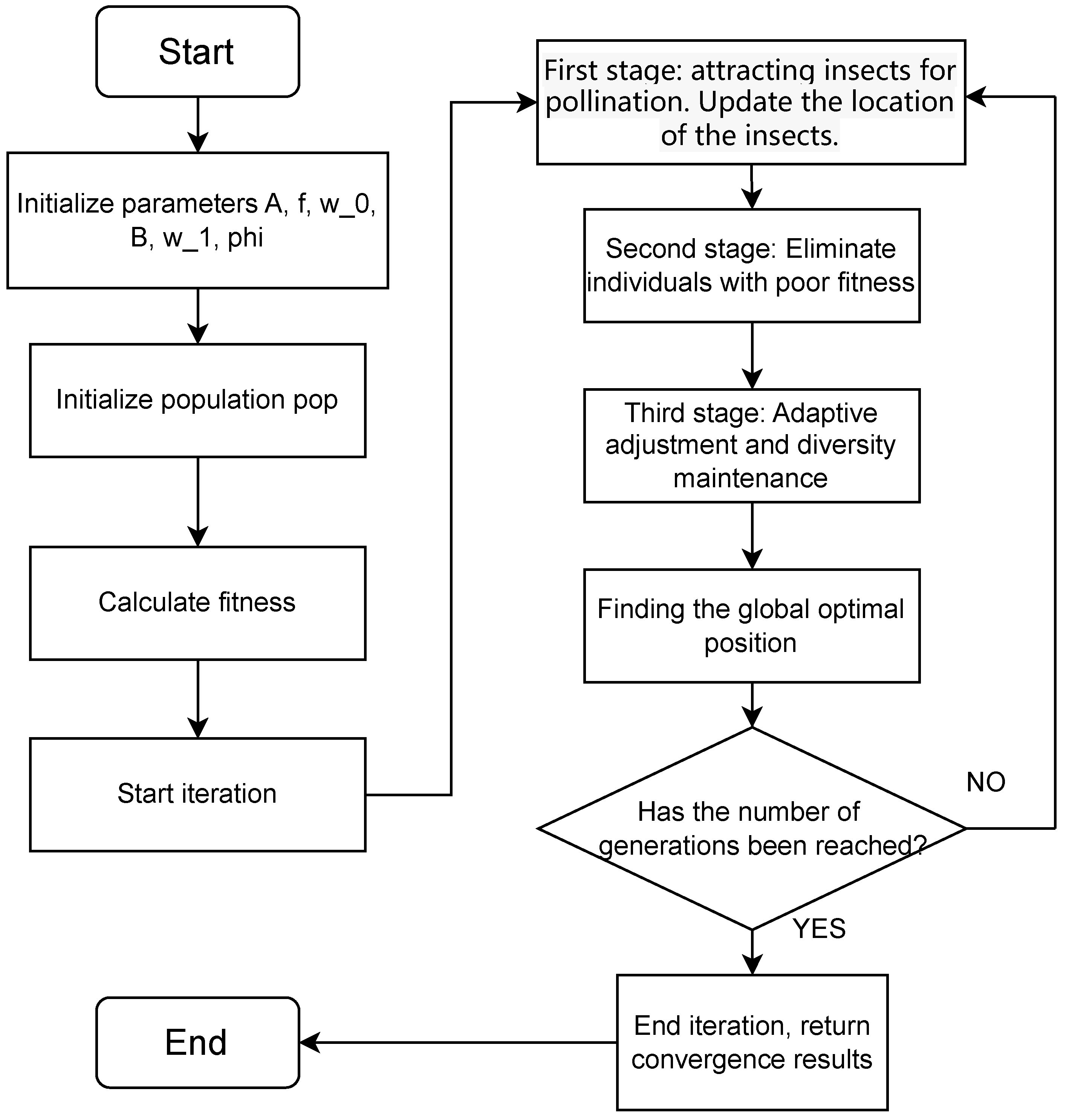
This paper investigates the Rafflesia optimization algorithm and its application to various engineering design problems. Broadly speaking, optimization is the process of finding the best solution from a range of possible choices. Within the contexts of mathematics and engineering, it typically involves maximizing or minimizing a specific function under given constraints.

Firstly, this work proposes the Diversity Maintenance Adaptive Rafflesia Optimization Algorithm as a novel approach for addressing these engineering design challenges. Through an Adaptive Weight Adjustment Strategy, the algorithm can dynamically alter the direction and intensity of the search, ensuring efficient search performance across various optimization stages. Additionally, the diversity maintenance strategy safeguards the diversity within the population, preventing the algorithm from prematurely settling into local optima. This implies that for engineering challenges such as spring design or gear system design, the algorithm can swiftly identify superior design solutions, which exhibit enhanced performance and reliability in practical applications. Furthermore, by benchmarking on the CEC2013 test functions, this paper further substantiates the superiority of the enhanced Rafflesia algorithm.

Secondly, the Adaptive Weight Adjustment Strategy, by automatically modulating the weights of the search strategy, can better adapt to different optimization problems and stages. When the algorithm ventures into a region of local optima, elevating the weight of global search assists the algorithm in escaping the local optimum to pursue improved solutions. To ensure population diversity and deter premature convergence, the maintenance of diversity within the population enables the algorithm to perpetually search on a global scale, amplifying its global optimization capabilities.

Thirdly, by incorporating biomimetic principles that consider the growth characteristics of the Rafflesia, the algorithm simulates its lifecycle from blooming to seed dispersion. This biomimetic approach furnishes the optimization algorithm with a fresh perspective, aligning the algorithm more closely with natural optimization mechanisms, thereby enhancing its efficiency and robustness. When compared to other algorithms, results from the CEC2013 benchmark test functions demonstrate that the new algorithm is not only theoretically distinct but also excels in practical applications. Particularly when juxtaposed against other mainstream optimization algorithms, the new method consistently outperforms across various evaluation metrics, solidifying its case for broader implementation in real-world engineering applications.

3. Method

This section primarily delves into the intricate details of the enhancements made to the AROA algorithm. It elucidates how the strategies employed within this improved algorithm confer it an edge over other optimization algorithms. The necessity of incorporating an adaptive weight updating strategy and a diversity maintenance strategy is also underscored.

3.1. Improvement Details

Comparing the original algorithm (ROA) with the newly enhanced version (AROA), several key modifications and refinements have been undertaken.

Firstly, the integration of an Adaptive Weight Adjustment Strategy has been introduced, primarily focusing on the third phase of the algorithm. A mechanism for adaptive weight adjustment has been newly added, allowing for dynamic updates of parameters such as $w_0$, $w_1$ and $phi$. This ensures that the algorithm’s movement within the search space is more flexible, allowing it to adjust its search strategy based on iteration counts. Such adjustments empower the algorithm with a robust global search capability in the early stages, followed by an efficient local search ability in the later stages, thereby enhancing its convergence rate.

Secondly, the inclusion of a diversity maintenance strategy has been made, with modifications also being made in the third phase of the algorithm. A similarity computation method has been introduced to assess if individuals within the population are overly alike. When two individuals are found to be too similar, one is reset. This strategy ensures the maintenance of diversity within the population, preventing the premature convergence to local optima.

Thirdly, probabilistic controls for weight adjustment and diversity maintenance have been implemented. Using the condition $ifrand<0.7$, weight adjustments and diversity maintenance are not conducted at every iteration. Instead, they are executed with a certain probability. This introduces an element of randomness to the algorithm, preventing premature convergence to a certain extent.

For a more in-depth understanding of the improvements, one can refer to the pseudocode of ROA labeled as Algorithm 1 and that of AROA depicted as Algorithm 2. Additionally, the flowchart in Figure 2 can also be consulted for further clarity.

3.1.1. Adaptive Weight Adjustment Improvement

Within the adaptive weight adjustment strategy, the initial focus revolves around the selection of weight parameters. The algorithm predominantly targets the adaptive adjustments of the weight parameters $w_0$, $w_1$ and $phi$. Weights hold significant importance in evolutionary algorithms given their capability to govern the direction and speed of the search process. To initialize the weight parameters, $w_0$ and $w_1$ are set to $1/f$, where f represents the wing-beat frequency. The $phi$ value is initialized to −0.78545.

As for the weight updating strategy, within the enhanced Rafflesia algorithm, the weight parameters are updated based on iteration count, denoted as $iter$, and the periodic parameter $pd$. An exponential decay strategy is employed for these updates, wherein the weights are diminished by multiplying them with an exponential function. This can be expressed through the subsequent formula:

$$w_0=w_0·\exp \left(-\frac{\mathrm{iter}-\frac{\mathrm{pd}}{2}}{\frac{\mathrm{pd}}{2}}\right)$$

(16)

$$w_1=w_1·\exp \left(-\frac{\mathrm{iter}-\frac{\mathrm{pd}}{2}}{\frac{\mathrm{pd}}{2}}\right)$$

(17)

$$phi=phi·\exp \left(-\frac{\mathrm{iter}-\frac{\mathrm{pd}}{2}}{\frac{\mathrm{pd}}{2}}\right)$$

(18)

The weight reduction strategy is devised based on the iteration number, represented as $iter$, and a periodic parameter, denoted as $pd$. As iterations progress, these weight parameters are methodically diminished, subsequently influencing the motion pattern of the insects. The behavior of insects in different phases is governed by these weight parameters. Both $w_0$ and $w_1$ are instrumental in striking a balance between the exploration and convergence of the insects, while $phi$ modulates the phase difference between the translational and rotational motions of the insects. Through variations in the fitness function, these parameters are adaptively set to influence the algorithm’s exploration and convergence performance. The frequency of weight parameter updates is regulated by the periodic parameter $pd$. In the presented algorithm, $pd$ orchestrates the updates of weight parameters, invoking a weight update operation whenever the condition $\mathrm{rem}(\mathrm{iter},\mathrm{pd})>\frac{\mathrm{pd}}{2}$ is met.

The weight parameters play a pivotal role in dictating the methodology of updating the insect’s position. This positional adjustment can be encapsulated by the subsequent formula for the first phase, which will be elaborated upon, where $target\_position$ is the target position and $random\_vector$ is the random vector. This formula elucidates how the insect’s position is adjusted based on the target and influenced by the random vector, modulated by the weight parameters.

$$\mathrm{new}\_\mathrm{position}=\mathrm{old}\_\mathrm{position}+w_0·(\mathrm{target}\_\mathrm{position}-\mathrm{old}\_\mathrm{position})+w_1·(\mathrm{random}\_\mathrm{vector}-0.5)+phi$$

(19)

3.1.2. Diversity Maintenance Improvement

The enhancements made to the algorithm also encompass the integration of a diversity maintenance strategy. The primary objective of this strategy is to uphold population diversity in each iteration, forestalling the algorithm from becoming ensnared in local optima, thereby augmenting its global search performance.

When refining the ROA with the Diversity Maintenance Strategy, a similarity threshold, denoted as $similarit{y}_{t}hreshold$, was initially defined. This threshold serves as a metric to gauge the similarity between individual entities within the population. A simplified form of the Euclidean distance was employed as the similarity measure. The formula for this similarity measure is presented as follows:

$$\mathrm{similarity}=\frac{1}{\dim }\sum _{k=1}^{\dim }\left|\mathrm{pop}(i,k)-\mathrm{pop}(j,k)\right|$$

(20)

In this context, $pop(i,k)$ and $pop(j,k)$ represent the position vectors of the i-th and j-th individuals within the population, respectively, while dimdim indicates the dimensionality of the problem. The similarity measure calculates the sum of the absolute differences between the dimensions of two individuals and then divides the result by the dimensionality, dimdim. Upon the computation of similarity, the algorithm embarks on the process of diversity maintenance. For each pair of individuals within the population, nested iterative loops ensure that each individual is juxtaposed against the rest. If the similarity, denoted as $similarity$, between two individuals exceeds the predefined similarity threshold, $similarity\_threshold$, diversity maintenance operations are executed. The condition for diversity maintenance can be articulated as $\mathrm{if}\mathrm{similarity}(i,j)>\mathrm{similarity}\_\mathrm{threshold}$.

Within the diversity maintenance operation, one individual, termed $rese{t}_{i}ndex$, is randomly chosen from the two similar entities. This selected individual is subsequently reverted to its initial state by invoking the $initialisation$ function to regenerate a random individual. This resetting maneuver enhances population diversity and furnishes the algorithm with the means to break free from local optima. The individual reset is characterized by

$$\mathrm{reset}\_\mathrm{index}=\mathrm{randi}\left(\right[i,j\left]\right)$$

(21)

$$\mathrm{pop}(\mathrm{reset}\_\mathrm{index},:)= \mathrm{random}\_\mathrm{initialization}\left(\right)$$

(22)

where $rando{m}_{i}nitialisation\left(\right)$ stands for a function devised to spawn a random individual. In essence, the Diversity Maintenance Strategy ensures population diversity by gauging inter-individual similarity and initiating an individual reset whenever similarity surpasses the set threshold. Such an approach augments the algorithm’s global search performance, curtailing the risks associated with premature convergence to local optima. This strategy proves invaluable across numerous optimization algorithms, especially when grappling with intricate problems.

Algorithm 2 The pseudo code of AROA.

1: // Third stage 2: if rem(iter, pd) > (pd / 2) then//rem denotes the remainder operation 3:      for i = 1 to sizepop do 4:          $rd\leftarrow \mathrm{rand}\times (ub-lb)+lb$ 5:          for j = 1 to dim do 6:              $pop(i,j)\leftarrow pop\_best\left(j\right)+rd\times \exp (\frac{iter}{Max\_iter}-1)\times \mathrm{sign}(\mathrm{rand}-0.5)$ 7:          end for 8:      end for 9:      if rand < 0.7 then 10:         // Update weights 11:         $w_0\leftarrow w_0\times \exp (-\frac{iter-\frac{pd}{2}}{\frac{pd}{2}})$                         ▹ Equation (16) 12:         $w_1\leftarrow w_1\times \exp (-\frac{iter-\frac{pd}{2}}{\frac{pd}{2}})$                         ▹ Equation (17) 13:         $\varphi \leftarrow \varphi \times \exp (-\frac{iter-\frac{pd}{2}}{\frac{pd}{2}})$                           ▹ Equation (18) 14:         // Diversity maintenance 15:         $similarity\_threshold\leftarrow 0.8$ 16:         for i = 1 to sizepop do 17:            for j = i + 1 to sizepop do 18:                $similarity\leftarrow \frac{{\sum }_{k=1}^{dim}\mathrm{abs}(pop(i,k)-pop(j,k))}{dim}$                   ▹ Equation (20) 19:                if $similarity>similarity\_threshold$ then 20:                    $reset\_index\leftarrow \mathrm{randi}\left(\right[i,j\left]\right)$                        ▹ Equation (21) 21:                    $pop(reset\_index,:)\leftarrow \mathrm{initialization}(1,dim,ub,lb)$        ▹ Equation (22) 22:                end if 23:            end for 24:         end for 25:     end if 26: end if

3.2. Role and Necessity of Strategy

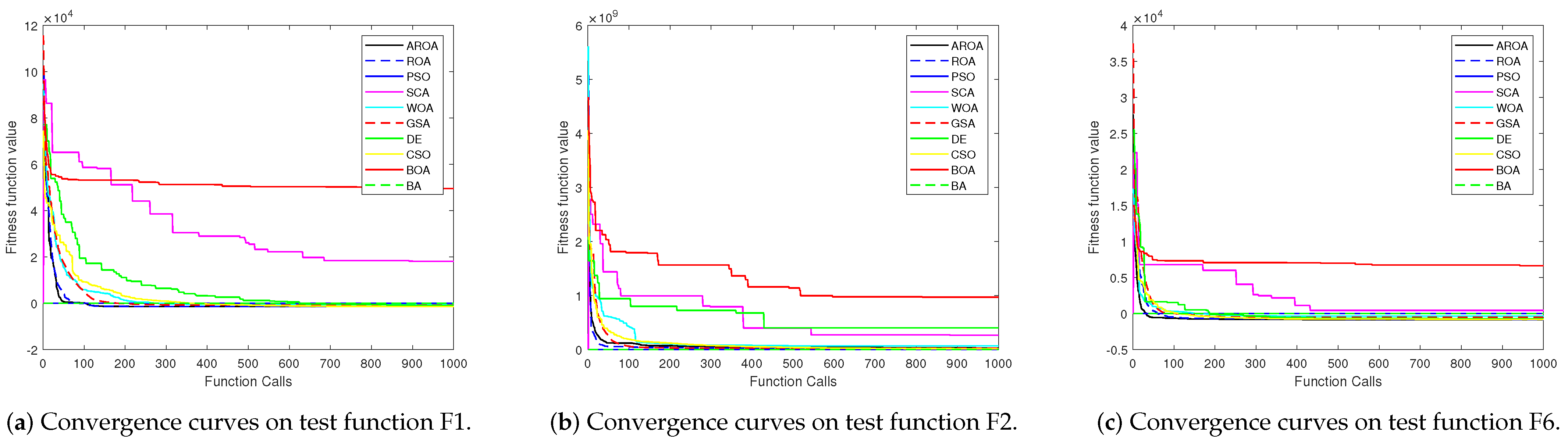
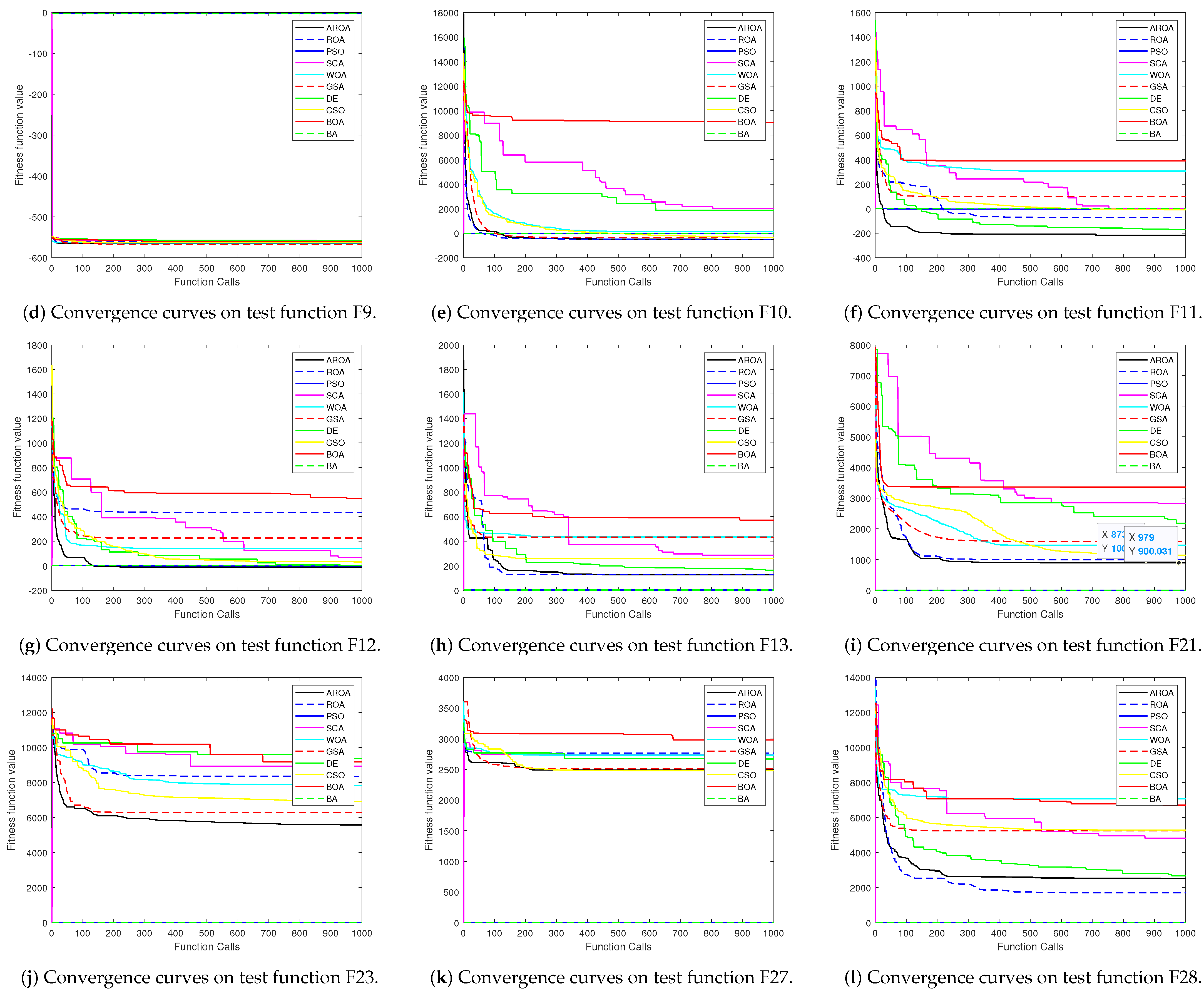
Adaptive weight adjustment fosters an improved balance between global and local searches within the algorithm, thereby amplifying the probability of pinpointing the global optimum. Diversity maintenance ensures adequate variation among individuals within the population, facilitating a more comprehensive exploration of the search space. This reduces the risk of entrapment in local optima at the expense of overlooking the global optimum. Through probabilistic control of weight adjustment and diversity maintenance, an element of randomness and unpredictability is injected into the algorithm, bolstering its robustness. With these enhancements, the novel optimization algorithm might, in certain scenarios, outstrip the original algorithm and other optimization techniques in terms of convergence speed and solution quality. Indeed, its efficacy has been corroborated using the CEC2013 benchmark function suite and in addressing specific engineering application problems.

To delve deeper, let us ponder over six distinct engineering applications and contemplate the potential advancements and superiority of AROA in these domains. In Section 5, this paper delineates several specific engineering applications, highlighting the treatment of varying constraint types. For instance, spring design might encompass different types of elasticity models and materials. Pressure vessel design may be riddled with myriad constraints, such as tensile strength and pressure endurance. Welded beam design might encompass constraints relating to weld strength and material durability, while gearbox design would perhaps necessitate considerations of multiple parameters and objectives. Gear system design could involve constraints on gear ratios and gear strength. AROA, through its adaptive weight adjustment strategy, can deftly adapt to these diverse design variables, ensuring all constraints are aptly met. Especially when grappling with tension/compression spring design, gearbox design, and the intricate design space commonly found in gearbox design, AROA’s integration of the diversity maintenance strategy amplifies its global search prowess. Endowed with a refined search mechanism, it evades premature local optima entrapment and sweeps the design space more exhaustively, tailoring its approach to the problem’s nuances. In these engineering realms, AROA’s enhancements might manifest as heightened adaptability, swifter convergence speeds, and superior global search capabilities, rendering it more adept at handling complex, multi-objective real-world engineering issues. The specific merits might necessitate validation through actual case studies and empirical results. Indeed, Section Five of this article provides a meticulous exposition of the experimental outcomes.

4. Experiments

The experimental section primarily entailed a performance assessment of the algorithm. In this evaluation, the algorithm was validated against the CEC2013 benchmark test suite. Finally, an analysis of the experimental data was completed.

4.1. Experiments Results

Testing was conducted using a 30-dimensional configuration, and the average fitness values (mean) and standard deviations (std) were documented after 30 independent runs of each algorithm. This approach provided a holistic assessment, affirming the efficacy of the newly proposed method. An additional tabular reference (

Table 1. Parameter settings for each related algorithm.

Algorithms	Parameter
AROA	N = 30, pd = Max_iter / 10; A = 2.5; f = 40; w_0 = 1 / f; B = 0.1;  w_1 = 1 / f; phi = −0.78545;
ROA	N = 30, pd = Max_iter / 10; A = 2.5; f = 40; w_0 = 1 / f; B = 0.1;  w_1 = 1 / f; phi = −0.78545;
PSO	N = 30, c = 2.0; w = 0.729; Vmax = 100; Vmin = −100;
WOA	N = 30;
GSA	N = 30, Rpower = 1; Rnorm = 2;
DE	N = 30; PCr = 0.5; F = 0.9;
CSO	N = 30; AP = 0.1; fl = 2;
BOA	N = 30; p = 0.6;  power_exponent = 0.1;  sensory_modality = 0.01;
BA	N = 30; r0 = 0.7; Af = 0.9; Rf = 0.9; Qmin = 0; Qmax = 1;
SCA	N = 30;

) was incorporated, detailing each algorithm under comparison, alongside their respective parameter settings. This augmentation was made to enhance the clarity and observability of the comparative framework.

Table 2. Assessment result 1.

Title	AROA’s Mean and Std Comparison Results with ROA, PSO, WOA, and GSA after Running 30 Times on CEC2013 Test Functions
Function	AROA Mean/std		ROA Mean/std		PSO Mean/std		WOA Mean/std		GSA Mean/std
f1	$-1.400\times {10}^3$	$1.019\times {10}^{-6}$	$-1.400\times {10}^3$	$2.351\times {10}^{-4}$	$-8.080\times {10}^2$	$2.301\times {10}^3$	$-8.762\times {10}^2$	$3.555\times {10}^2$	$-1.387\times {10}^3$	$9.374\times {10}^1$
f2	$1.674\times {10}^7$	$1.502\times {10}^6$	$1.245\times {10}^7$	$1.184\times {10}^6$	$1.687\times {10}^7$	$2.864\times {10}^7$	$3.188\times {10}^7$	$3.817\times {10}^7$	$3.283\times {10}^7$	$6.318\times {10}^6$
f3	$4.333\times {10}^9$	$1.450\times {10}^9$	$4.949\times {10}^9$	$1.602\times {10}^9$	$4.471\times {10}^9$	$1.043\times {10}^{11}$	$1.062\times {10}^{10}$	$5.003\times {10}^{10}$	$1.293\times {10}^{13}$	$9.451\times {10}^{13}$
f4	$7.007\times {10}^4$	$1.679\times {10}^3$	$7.452\times {10}^4$	$1.047\times {10}^4$	$7.867\times {10}^4$	$2.062\times {10}^4$	$4.689\times {10}^4$	$2.212\times {10}^4$	$7.191\times {10}^4$	$5.085\times {10}^3$
f5	$-9.901\times {10}^2$	$2.848\times {10}^0$	$-9.992\times {10}^2$	$9.009\times {10}^{-4}$	$-9.894\times {10}^2$	$1.762\times {10}^3$	$4.392\times {10}^2$	$2.849\times {10}^2$	$-3.571\times {10}^2$	$2.280\times {10}^2$
f6	$-8.805\times {10}^2$	$9.938\times {10}^0$	$-8.416\times {10}^2$	$2.713\times {10}^1$	$-8.209\times {10}^2$	$5.122\times {10}^2$	$-7.208\times {10}^2$	$1.156\times {10}^2$	$-5.133\times {10}^2$	$8.256\times {10}^2$
f7	$-6.244\times {10}^2$	$1.332\times {10}^1$	$-6.147\times {10}^2$	$2.592\times {10}^1$	$-6.254\times {10}^2$	$3.292\times {10}^1$	$-7.223\times {10}^2$	$1.797\times {10}^3$	$4.376\times {10}^3$	$5.199\times {10}^3$
f8	$-6.790\times {10}^2$	$1.449\times {10}^{-2}$	$-6.789\times {10}^2$	$6.209\times {10}^{-2}$	$-6.790\times {10}^2$	$3.284\times {10}^{-2}$	$-6.790\times {10}^2$	$9.453\times {10}^{-2}$	$-6.790\times {10}^2$	$4.474\times {10}^{-2}$
f9	$-5.693\times {10}^2$	$2.191\times {10}^0$	$-5.644\times {10}^2$	$1.546\times {10}^0$	$-5.631\times {10}^2$	$2.203\times {10}^{-1}$	$-5.775\times {10}^2$	$1.244\times {10}^0$	$-5.630\times {10}^2$	$3.024\times {10}^0$
f10	$-4.905\times {10}^2$	$1.860\times {10}^0$	$-4.962\times {10}^2$	$2.839\times {10}^0$	$-4.911\times {10}^2$	$7.484\times {10}^2$	$-1.340\times {10}^2$	$1.667\times {10}^2$	$-2.065\times {10}^2$	$1.705\times {10}^2$
f11	$-3.075\times {10}^1$	$6.542\times {10}^1$	$4.459\times {10}^1$	$2.526\times {10}^2$	$-6.964\times {10}^{-1}$	$6.575\times {10}^1$	$-2.717\times {10}^2$	$6.812\times {10}^1$	$5.864\times {10}^1$	$2.546\times {10}^1$
f12	$9.651\times {10}^1$	$9.620\times {10}^1$	$1.801\times {10}^2$	$1.224\times {10}^2$	$1.075\times {10}^2$	$9.883\times {10}^1$	$-1.220\times {10}^2$	$1.322\times {10}^2$	$2.464\times {10}^2$	$9.036\times {10}^1$
f13	$2.109\times {10}^2$	$8.637\times {10}^1$	$1.928\times {10}^2$	$6.228\times {10}^1$	$2.107\times {10}^2$	$3.399\times {10}^1$	$3.677\times {10}^2$	$2.510\times {10}^1$	$4.740\times {10}^2$	$8.296\times {10}^1$
f14	$4.273\times {10}^3$	$2.557\times {10}^2$	$4.842\times {10}^3$	$5.817\times {10}^2$	$4.104\times {10}^3$	$9.185\times {10}^2$	$4.700\times {10}^3$	$1.243\times {10}^3$	$4.042\times {10}^3$	$7.894\times {10}^2$
f15	$5.052\times {10}^3$	$8.422\times {10}^2$	$5.141\times {10}^3$	$5.472\times {10}^2$	$5.034\times {10}^3$	$7.398\times {10}^2$	$6.796\times {10}^3$	$6.856\times {10}^2$	$4.164\times {10}^3$	$4.034\times {10}^2$
f16	$2.017\times {10}^2$	$1.251\times {10}^{-1}$	$2.018\times {10}^2$	$4.934\times {10}^{-1}$	$2.019\times {10}^2$	$2.589\times {10}^{-1}$	$2.031\times {10}^2$	$4.220\times {10}^{-1}$	$2.001\times {10}^2$	$9.824\times {10}^{-3}$
f17	$8.016\times {10}^2$	$1.781\times {10}^1$	$7.657\times {10}^2$	$9.839\times {10}^1$	$8.041\times {10}^2$	$1.602\times {10}^2$	$5.307\times {10}^2$	$6.321\times {10}^1$	$5.902\times {10}^2$	$4.096\times {10}^1$
f18	$-1.400\times {10}^3$	$1.234\times {10}^2$	$-1.400\times {10}^3$	$6.813\times {10}^1$	$-1.400\times {10}^3$	$1.521\times {10}^2$	$-1.400\times {10}^3$	$3.373\times {10}^1$	$-1.400\times {10}^3$	$3.636\times {10}^1$
f19	$5.376\times {10}^2$	$2.506\times {10}^0$	$5.354\times {10}^2$	$1.096\times {10}^1$	$5.411\times {10}^2$	$1.258\times {10}^4$	$7.718\times {10}^2$	$2.636\times {10}^2$	$8.160\times {10}^2$	$1.041\times {10}^2$
f20	$6.141\times {10}^2$	$3.202\times {10}^{-1}$	$6.148\times {10}^2$	$0.000\times {10}^0$	$6.143\times {10}^2$	$2.859\times {10}^{-1}$	$6.150\times {10}^2$	$2.070\times {10}^{-1}$	$6.150\times {10}^2$	$0.000\times {10}^0$
f21	$9.921\times {10}^2$	$1.015\times {10}^2$	$1.010\times {10}^3$	$1.011\times {10}^2$	$1.022\times {10}^3$	$5.158\times {10}^2$	$1.966\times {10}^3$	$9.324\times {10}^1$	$1.802\times {10}^3$	$3.018\times {10}^2$
f22	$6.094\times {10}^3$	$1.778\times {10}^2$	$7.029\times {10}^3$	$2.347\times {10}^3$	$6.695\times {10}^3$	$6.135\times {10}^2$	$4.935\times {10}^3$	$1.091\times {10}^3$	$7.558\times {10}^3$	$5.074\times {10}^2$
f23	$6.744\times {10}^3$	$3.037\times {10}^2$	$6.830\times {10}^3$	$1.250\times {10}^2$	$7.040\times {10}^3$	$5.494\times {10}^2$	$5.966\times {10}^3$	$9.310\times {10}^2$	$7.168\times {10}^3$	$3.226\times {10}^2$
f24	$1.309\times {10}^3$	$1.512\times {10}^{-1}$	$1.312\times {10}^3$	$2.055\times {10}^1$	$1.310\times {10}^3$	$9.063\times {10}^0$	$1.261\times {10}^3$	$9.877\times {10}^0$	$1.475\times {10}^3$	$2.512\times {10}^1$
f25	$1.423\times {10}^3$	$4.902\times {10}^0$	$1.426\times {10}^3$	$1.610\times {10}^1$	$1.423\times {10}^3$	$6.504\times {10}^0$	$1.434\times {10}^3$	$1.388\times {10}^1$	$1.517\times {10}^3$	$4.805\times {10}^0$
f26	$1.401\times {10}^3$	$1.252\times {10}^{-1}$	$1.569\times {10}^3$	$1.125\times {10}^{-1}$	$1.401\times {10}^3$	$5.385\times {10}^0$	$1.513\times {10}^3$	$8.005\times {10}^0$	$1.600\times {10}^3$	$6.586\times {10}^1$
f27	$2.553\times {10}^3$	$3.378\times {10}^1$	$2.586\times {10}^3$	$1.570\times {10}^2$	$2.609\times {10}^3$	$5.054\times {10}^1$	$2.581\times {10}^3$	$9.709\times {10}^1$	$2.534\times {10}^3$	$1.671\times {10}^2$
f28	$3.934\times {10}^3$	$4.812\times {10}^1$	$2.436\times {10}^3$	$2.133\times {10}^3$	$3.893\times {10}^3$	$1.410\times {10}^3$	$2.967\times {10}^3$	$6.269\times {10}^2$	$5.766\times {10}^3$	$4.762\times {10}^2$
win	-		20	-	19	-	17	-	21	-
Description	“win” quantifies the number of times AROA outperformed its competitors in terms of the evaluation metric “Mean”

and

Table 3. Assessment result 2.

Title	AROA’s Mean and Std Comparison Results with DE, CSO, BOA, BA, and SCA after Running 30 Times on CEC2013 Test Functions.
Function	DE Mean/Std		CSO Mean/Std		BOA Mean/Std		BA Mean/Std		SCA Mean/Std
f1	$-7.661\times {10}^2$	$1.092\times {10}^2$	$-1.393\times {10}^3$	$1.567\times {10}^1$	$4.925\times {10}^4$	$3.577\times {10}^3$	$-1.394\times {10}^3$	$7.706\times {10}^{-1}$	$1.308\times {10}^4$	$2.429\times {10}^3$
f2	$3.607\times {10}^8$	$6.874\times {10}^7$	$2.329\times {10}^7$	$1.225\times {10}^7$	$8.454\times {10}^8$	$5.469\times {10}^8$	$6.033\times {10}^6$	$2.581\times {10}^6$	$2.614\times {10}^8$	$1.864\times {10}^7$
f3	$2.164\times {10}^{10}$	$4.806\times {10}^9$	$1.191\times {10}^{10}$	$4.578\times {10}^9$	$9.954\times {10}^{20}$	$6.171\times {10}^{19}$	$5.981\times {10}^8$	$1.393\times {10}^9$	$1.179\times {10}^{11}$	$2.627\times {10}^{10}$
f4	$1.418\times {10}^5$	$1.837\times {10}^4$	$3.187\times {10}^4$	$6.877\times {10}^3$	$5.622\times {10}^4$	$6.599\times {10}^3$	$9.798\times {10}^4$	$3.502\times {10}^4$	$5.223\times {10}^4$	$2.740\times {10}^3$
f5	$-9.413\times {10}^2$	$7.524\times {10}^0$	$-7.880\times {10}^2$	$5.554\times {10}^1$	$2.607\times {10}^4$	$1.130\times {10}^4$	$-9.977\times {10}^2$	$2.820\times {10}^{-1}$	$2.522\times {10}^3$	$7.964\times {10}^2$
f6	$-7.180\times {10}^2$	$1.962\times {10}^1$	$-7.569\times {10}^2$	$4.606\times {10}^1$	$1.149\times {10}^4$	$2.180\times {10}^3$	$-8.529\times {10}^2$	$2.670\times {10}^1$	$5.368\times {10}^2$	$2.494\times {10}^2$
f7	$-6.447\times {10}^2$	$1.926\times {10}^1$	$-6.277\times {10}^2$	$4.571\times {10}^1$	$6.423\times {10}^5$	$4.454\times {10}^6$	$1.353\times {10}^6$	$5.606\times {10}^5$	$-5.184\times {10}^2$	$4.736\times {10}^1$
f8	$-6.789\times {10}^2$	$5.789\times {10}^{-2}$	$-6.789\times {10}^2$	$3.649\times {10}^{-2}$	$-6.790\times {10}^2$	$6.249\times {10}^{-2}$	$-6.789\times {10}^2$	$5.445\times {10}^{-2}$	$-6.789\times {10}^2$	$8.050\times {10}^{-2}$
f9	$-5.582\times {10}^2$	$1.167\times {10}^0$	$-5.659\times {10}^2$	$1.881\times {10}^0$	$-5.603\times {10}^2$	$1.489\times {10}^0$	$-5.609\times {10}^2$	$3.522\times {10}^0$	$-5.583\times {10}^2$	$9.072\times {10}^{-1}$
f10	$1.264\times {10}^3$	$3.653\times {10}^2$	$-3.626\times {10}^2$	$9.060\times {10}^1$	$8.269\times {10}^3$	$1.918\times {10}^3$	$-4.973\times {10}^2$	$4.770\times {10}^{-1}$	$1.930\times {10}^3$	$6.819\times {10}^2$
f11	$-1.958\times {10}^2$	$1.673\times {10}^1$	$-5.594\times {10}^1$	$5.828\times {10}^1$	$4.037\times {10}^2$	$7.406\times {10}^1$	$5.029\times {10}^2$	$2.096\times {10}^2$	$4.082\times {10}^1$	$4.233\times {10}^1$
f12	$2.018\times {10}^1$	$1.680\times {10}^1$	$2.674\times {10}^1$	$7.685\times {10}^1$	$5.077\times {10}^2$	$6.738\times {10}^1$	$5.689\times {10}^2$	$1.327\times {10}^2$	$1.382\times {10}^2$	$2.003\times {10}^1$
f13	$1.161\times {10}^2$	$1.645\times {10}^1$	$1.871\times {10}^2$	$5.751\times {10}^1$	$5.863\times {10}^2$	$4.375\times {10}^1$	$7.715\times {10}^2$	$1.297\times {10}^2$	$2.434\times {10}^2$	$3.819\times {10}^1$
f14	$4.478\times {10}^3$	$2.300\times {10}^2$	$4.411\times {10}^3$	$5.923\times {10}^2$	$7.946\times {10}^3$	$5.364\times {10}^2$	$5.035\times {10}^3$	$8.332\times {10}^2$	$7.328\times {10}^3$	$3.995\times {10}^2$
f15	$8.089\times {10}^3$	$3.666\times {10}^2$	$4.172\times {10}^3$	$6.122\times {10}^2$	$8.061\times {10}^3$	$2.095\times {10}^2$	$5.352\times {10}^3$	$6.707\times {10}^2$	$8.033\times {10}^3$	$3.994\times {10}^2$
f16	$2.031\times {10}^2$	$3.598\times {10}^{-1}$	$2.013\times {10}^2$	$6.950\times {10}^{-1}$	$2.032\times {10}^2$	$2.713\times {10}^{-1}$	$2.027\times {10}^2$	$3.775\times {10}^{-1}$	$2.030\times {10}^2$	$4.818\times {10}^{-1}$
f17	$6.364\times {10}^2$	$5.173\times {10}^1$	$6.294\times {10}^2$	$5.982\times {10}^1$	$1.149\times {10}^3$	$3.023\times {10}^1$	$1.815\times {10}^3$	$2.222\times {10}^2$	$8.932\times {10}^2$	$5.558\times {10}^1$
f18	$8.145\times {10}^2$	$4.821\times {10}^1$	$6.708\times {10}^2$	$4.541\times {10}^1$	$1.236\times {10}^3$	$5.412\times {10}^1$	$1.960\times {10}^3$	$1.643\times {10}^2$	$9.955\times {10}^2$	$4.659\times {10}^1$
f19	$5.911\times {10}^2$	$3.396\times {10}^1$	$5.307\times {10}^2$	$1.013\times {10}^1$	$5.005\times {10}^5$	$1.681\times {10}^5$	$5.437\times {10}^2$	$7.380\times {10}^0$	$1.293\times {10}^4$	$1.889\times {10}^4$
f20	$6.137\times {10}^2$	$2.061\times {10}^{-1}$	$6.143\times {10}^2$	$1.552\times {10}^{-1}$	$6.150\times {10}^2$	$4.130\times {10}^{-6}$	$6.150\times {10}^2$	$0.000\times {10}^0$	$6.145\times {10}^2$	$1.577\times {10}^{-1}$
f21	$2.037\times {10}^3$	$2.694\times {10}^2$	$1.105\times {10}^3$	$7.157\times {10}^1$	$3.173\times {10}^3$	$7.168\times {10}^1$	$1.069\times {10}^3$	$8.736\times {10}^1$	$2.820\times {10}^3$	$3.430\times {10}^1$
f22	$6.531\times {10}^3$	$4.574\times {10}^2$	$6.492\times {10}^3$	$3.973\times {10}^2$	$9.446\times {10}^3$	$3.506\times {10}^2$	$7.471\times {10}^3$	$9.922\times {10}^2$	$8.990\times {10}^3$	$4.800\times {10}^2$
f23	$9.161\times {10}^3$	$1.693\times {10}^2$	$6.798\times {10}^3$	$9.760\times {10}^2$	$9.653\times {10}^3$	$3.784\times {10}^2$	$7.321\times {10}^3$	$9.536\times {10}^2$	$9.255\times {10}^3$	$2.418\times {10}^2$
f24	$1.309\times {10}^3$	$2.748\times {10}^0$	$1.321\times {10}^3$	$1.405\times {10}^1$	$1.376\times {10}^3$	$3.195\times {10}^1$	$1.379\times {10}^3$	$5.038\times {10}^1$	$1.326\times {10}^3$	$6.262\times {10}^0$
f25	$1.413\times {10}^3$	$4.366\times {10}^0$	$1.459\times {10}^3$	$1.919\times {10}^1$	$1.440\times {10}^3$	$1.600\times {10}^1$	$1.397\times {10}^3$	$6.761\times {10}^0$	$1.438\times {10}^3$	$4.150\times {10}^0$
f26	$1.551\times {10}^3$	$5.321\times {10}^1$	$1.419\times {10}^3$	$5.363\times {10}^1$	$1.467\times {10}^3$	$6.059\times {10}^1$	$1.582\times {10}^3$	$9.942\times {10}^1$	$1.433\times {10}^3$	$4.584\times {10}^0$
f27	$2.675\times {10}^3$	$3.282\times {10}^1$	$2.509\times {10}^3$	$1.443\times {10}^2$	$3.070\times {10}^3$	$1.056\times {10}^2$	$2.769\times {10}^3$	$1.238\times {10}^2$	$2.727\times {10}^3$	$5.072\times {10}^1$
f28	$2.744\times {10}^3$	$1.269\times {10}^2$	$4.797\times {10}^3$	$1.482\times {10}^3$	$6.663\times {10}^3$	$3.937\times {10}^2$	$7.739\times {10}^3$	$1.113\times {10}^3$	$4.617\times {10}^3$	$1.987\times {10}^2$
win	18	-	17	-	27	-	23	-	27	-
Description	“win” quantifies the number of times AROA outperformed its competitors in terms of the evaluation metric “Mean”

showcase the statistical outcomes for each algorithm. At the conclusion of each table, the term “win” quantifies the number of occasions on which the AROA surpassed its competitors in terms of the evaluation metric “Mean”. From the data presented in these tables, it can be observed that AROA exhibited superior performance in terms of both average fitness values (mean) and standard deviations (std).

This study juxtaposed the enhanced algorithm, AROA, with its predecessor, ROA, while also drawing comparisons with eight other optimization algorithms. These encompass the Particle Swarm Optimization (PSO), Whale Optimization Algorithm (WOA), Gravitational Search Algorithm (GSA), Differential Evolution (DE), Cat Swarm Optimization (CSO), Butterfly Optimization Algorithm (BOA), Bat Algorithm (BA), and the Sine Cosine Algorithm (SCA).

All experiments were conducted using MATLAB 2021a software. For algorithm evaluation, the $CEC2013$ [27] benchmark test functions were employed to assess the performance of AROA. The $CEC2013$ [28] test function set serves as a standard benchmark for evaluating the efficacy of optimization algorithms. Comprising 28 distinct test functions, the suite encompasses unimodal, multimodal, and some intricate test functions. These are designed to simulate various types of optimization problems, ensuring a comprehensive appraisal of an algorithm’s capabilities. Throughout the testing procedure, the dimensionality of the test functions was set at $D=30$. Consistent parameter settings were maintained, with a population size of N (where $(N=30)$), and the evaluation was executed 1000 times for the algorithm.

Table 2 and Table 3 present the results of the algorithm on the test function suite. A comparative assessment, based on the average values obtained after 30 independent runs, revealed performance differences between AROA, ROA, and nine other intelligent optimization algorithms. As depicted in the data, the AROA algorithm outperformed the ROA algorithm on 20 of the CEC2013 test functions, predominantly emerging superior. Comparable results were observed for the functions $F5$, $F10$, $F16$, $F19$ and $F20$. When pitted against the PSO algorithm, AROA outshone in 19 test functions. Against WOA, AROA excelled in 17 test functions. AROA demonstrated superior performance in 21 functions when contrasted with GSA and in 17 functions each against DE and CSO. In comparisons with BOA and SCA, AROA prevailed in 27 functions and outperformed BA in 23 functions. Collectively, this assessment underscores AROA’s enhanced performance across the test functions.

To offer a more discernible visualization of the experimental outcomes, convergence curves were plotted for a random selection of three diverse function types (unimodal, multimodal, and complex). Twelve test functions were selected: F1, F2, F6, F9, F10, F11, F12, F13, F21, F23, F27, and F28. The graphical depictions of these convergence outcomes are presented in Figure 3a–l.

4.2. Experimental Analysis

Upon analyzing the experimental data, it can be discerned that the integration of Adaptive Weight Updating and Diversity Maintenance Strategies typically exerts a positive influence on algorithmic performance.

Primarily, the Diversity Maintenance Strategy enhances particle diversity. When an algorithm maintains a diverse particle swarm, it is more apt to encompass a larger search space. This proves particularly beneficial in circumventing local optima and potentially discovering the global optimum.

Additionally, adaptive weight updates facilitate exploration during the algorithm’s early stages. Broad-ranging searches, or exploration, are paramount in these initial phases. Such a strategy ensures that the algorithm does not become confined to a specific region prematurely, granting it the opportunity to discern promising regions within the entirety of the search space. This aspect becomes particularly salient when scrutinized alongside specific CEC2013 test functions.

For unimodal problems, adaptive weight updating aids the algorithm in swiftly pinpointing the global optimum. During the algorithm’s nascent stages, a preference for higher weight values is observed to boost exploration. As iterations increase, this weight gradually diminishes, accentuating exploitation and steering the algorithm closer to the global optimum. Even though the search space of unimodal problems is relatively straightforward, retaining diversity is essential to ensure the algorithm does not succumb prematurely to potential local optima or suboptimal zones.

The complexity of multimodal problems stems from the presence of numerous local optima. In the early stages, a substantial weight is required for extensive exploration. As the algorithm progresses, the weight may gradually decrease. Adaptive weight updating assists the algorithm in conducting precise searches within discerned peak regions. Thus, in multimodal problems, maintaining diversity is pivotal. It ensures that the algorithm comprehensively scours the search space and does not become easily enamored by local optima.

Complex functions may exhibit diverse characteristics, such as local optima, plateaus, peaks, and valleys. Adaptive weight updating enables the algorithm to adapt to these features at various stages, broadly exploring initially and conducting precise searches in promising regions later on. To eschew complexity pitfalls, upholding diversity ensures the algorithm does not become ensnared within any specific region throughout the search, retaining the potential to unearth novel, promising areas.

In summation, the inclusion of adaptive weight updating and diversity maintenance strategies empowers the algorithm to adeptly balance exploration and exploitation, resulting in enhanced performance across diverse problem types. For unimodal problems, the algorithm can identify the global optimum more swiftly. In the context of multimodal and complex functions, the algorithm is less prone to being trapped in local optima, having a heightened chance of locating the global optimum. To vividly illustrate convergence efficacy, we have also selected several illustrative convergence plots from each category of test functions for display.

5. Application

This section predominantly elucidates the contextual relationship between the ROA and other metaheuristic algorithms with engineering optimization problems. A comparative performance evaluation of various algorithms across six distinct engineering optimization problems is undertaken, followed by an analytical appraisal of the gathered data.

5.1. Application Background

Metaheuristic algorithms emulate the evolutionary processes observed in nature. These algorithms are conceived through observing behaviors in nature and abstracting them into computational methodologies. Natural evolution has been proven to be an effective optimization process; thus, leveraging these strategies to address engineering challenges becomes intuitively appealing. In terms of search capabilities, nature-inspired algorithms are often endowed with robust global search abilities. This suggests that they can explore various regions of the solution space without easily succumbing to local optima. Such a capability is paramount for specific engineering optimization problems, given that they frequently exhibit multiple local optima and intricate search spaces. Metaheuristic algorithms, aptly equipped in this domain, proffer an efficacious approach. Pertaining to adaptability, metaheuristic algorithms typically demonstrate high adaptability. This denotes their capacity to self-adjust to tackle disparate problems and dynamic environments. In engineering optimization, this becomes a salient trait, as real-world problems can evolve over time. Addressing multi-objectivity and constraint handling, myriad engineering challenges are multi-objective and encompass diverse constraints. Nature-inspired algorithms often incorporate inherent mechanisms to manage these multi-objectives and constraints, rendering them ideal solutions for such quandaries. In practical engineering problem solving, due to their intuitive and flexible nature, these nature-inspired algorithms have been successfully applied across various real-world engineering domains, ranging from aerospace engineering to power system optimization.

The ROA algorithm, introduced herein, is inspired by the pollen dissemination mechanism. This mechanism permits the algorithm to extensively scour the solution space, enhancing its likelihood of pinpointing the global optimum. Moreover, the ROA algorithm can be seamlessly extended to multi-objective optimization problems, concurrently handling multiple constraints. It contemplates multiple objectives and identifies solutions that satisfy all constraints. The advanced version, AROA, as iterations unfold, can autonomously adjust its search strategy and adaptively update weights, thereby seeking optimal solutions more efficiently. Furthermore, the algorithm is not reliant on specific problem characteristics, bestowing it with commendable versatility, making it apt for a gamut of engineering optimization challenges. Conclusively, leveraging the attributes of the King Protea Optimization Algorithm, its integration with engineering optimization challenges can substantially aid in discerning optimal solutions.

5.2. Applied Experiments

For the initial five engineering applications, the performance of the Enhanced Rafflesia Optimization Algorithm (AROA), the original Rafflesia Optimization Algorithm [29] (ROA), Whale Optimization Algorithm (WOA), Grey Wolf Optimizer (GWO), Harris Hawk Optimizer [30] (HHO), and Osprey Optimization Algorithm [31] (OOA) were assessed. The evaluation results are delineated in Table 1. For the sixth engineering application [32], the performance of the Enhanced Rafflesia Optimisation Algorithm (AROA), the original Rafflesia Optimisation Algorithm (ROA), Grey Wolf Optimizer (GWO), Dung Beetle Optimizer [33] (DBO), Dandelion Optimization [34] (DO), Harris Hawk Optimizer (HHO), and Snake Swarm Optimization [35,36] (SO) were evaluated.

In each engineering application, the efficacy of the novel algorithm (AROA) was gauged by contrasting its optimal values against those derived from other algorithms. In this segment, a total of 12 tabulated datasets are provided, detailing the constraints and objective functions for six engineering application problems, along with the optimal values obtained by various algorithms across these six applications, as portrayed in Table 4, Table 5, Table 6, Table 7, Table 8, Table 9, Table 10, Table 11, Table 12, Table 13, Table 14 and Table 15. Through a close inspection of the optimal values, it was discerned that the AROA algorithm frequently surpassed its counterparts, thereby underscoring its superior performance in practical applications.

Table 4. Engineering optimization problem 1.

Name	Function
Consider	$x=\left[x_1{x}_2{x}_3\right]$ = [d D N]
Minimize	$f\left(x\right)=(x_3+2)·x_2·\left(x_1^2\right)$
Subject to	$g_1\left(x\right)=1-\frac{\left(x_2^3\right)·x_3}{71785·\left(x_1^4\right)}\le 0$
	$g_2\left(x\right)=\frac{4·\left(x_2^2\right)-x_1·x_2}{12566·(x_2·\left(x_1^3\right)-\left(x_1^4\right))}+\frac{1}{5108·\left(x_1^2\right)}-1\le 0$
	$g_3\left(x\right)=1-\frac{140.45·x_1}{\left(x_2^2\right)·x_3}\le 0$
	$g_4\left(x\right)=\frac{(x_1+x_2)}{1.5}-1\le 0$
Parametersrange	0.05 ≤  $x_1$ ≤ 2, 0.25 ≤ $x_2$ ≤ 1.3, 2 ≤ $x_3$ ≤ 15

Table 4. Engineering optimization problem 1.

Name	Function
Consider	$x=\left[x_1{x}_2{x}_3\right]$ = [d D N]
Minimize	$f\left(x\right)=(x_3+2)·x_2·\left(x_1^2\right)$
Subject to	$g_1\left(x\right)=1-\frac{\left(x_2^3\right)·x_3}{71785·\left(x_1^4\right)}\le 0$
	$g_2\left(x\right)=\frac{4·\left(x_2^2\right)-x_1·x_2}{12566·(x_2·\left(x_1^3\right)-\left(x_1^4\right))}+\frac{1}{5108·\left(x_1^2\right)}-1\le 0$
	$g_3\left(x\right)=1-\frac{140.45·x_1}{\left(x_2^2\right)·x_3}\le 0$
	$g_4\left(x\right)=\frac{(x_1+x_2)}{1.5}-1\le 0$
Parametersrange	0.05 ≤  $x_1$ ≤ 2, 0.25 ≤ $x_2$ ≤ 1.3, 2 ≤ $x_3$ ≤ 15

Table 5. Engineering optimization problem 1 results.

Algorithm	${\mathit{x}}_1$	${\mathit{x}}_2$	${\mathit{x}}_3$	fbest
WOA	$5.890\times {10}^{-2}$	$5.563\times {10}^{-1}$	$5.018\times {10}^0$	$1.355\times {10}^{-2}$
HHO	$5.000\times {10}^{-2}$	$3.137\times {10}^{-1}$	$1.453\times {10}^1$	$1.297\times {10}^{-2}$
GWO	$5.000\times {10}^{-2}$	$3.173\times {10}^{-1}$	$1.406\times {10}^1$	$1.274\times {10}^{-2}$
OOA	$5.659\times {10}^{-2}$	$4.865\times {10}^{-1}$	$6.398\times {10}^0$	$1.308\times {10}^{-2}$
AROA	$5.089\times {10}^{-2}$	$3.377\times {10}^{-1}$	$1.250\times {10}^1$	$1.268\times {10}^{-2}$
ROA	$6.257\times {10}^{-2}$	$6.791\times {10}^{-1}$	$3.516\times {10}^0$	$1.466\times {10}^{-2}$

Table 5. Engineering optimization problem 1 results.

Algorithm	${\mathit{x}}_1$	${\mathit{x}}_2$	${\mathit{x}}_3$	fbest
WOA	$5.890\times {10}^{-2}$	$5.563\times {10}^{-1}$	$5.018\times {10}^0$	$1.355\times {10}^{-2}$
HHO	$5.000\times {10}^{-2}$	$3.137\times {10}^{-1}$	$1.453\times {10}^1$	$1.297\times {10}^{-2}$
GWO	$5.000\times {10}^{-2}$	$3.173\times {10}^{-1}$	$1.406\times {10}^1$	$1.274\times {10}^{-2}$
OOA	$5.659\times {10}^{-2}$	$4.865\times {10}^{-1}$	$6.398\times {10}^0$	$1.308\times {10}^{-2}$
AROA	$5.089\times {10}^{-2}$	$3.377\times {10}^{-1}$	$1.250\times {10}^1$	$1.268\times {10}^{-2}$
ROA	$6.257\times {10}^{-2}$	$6.791\times {10}^{-1}$	$3.516\times {10}^0$	$1.466\times {10}^{-2}$

5.2.1. Tension/Compression Spring Design Problems

The design of tension and compression springs [37,38] is a pivotal concern within the realm of engineering optimization. Such challenges encompass the design and optimization of springs utilized for regulating force, displacement, or energy to meet specific performance and constraint demands inherent to certain engineering applications. These springs find extensive deployment across diverse sectors, including automotive suspension systems, architectural structures, mechanical apparatuses, and electronic devices.

In addressing the tension/compression spring design quandary, engineers are initially compelled to select an apt spring material. This selection process is intrinsically governed by considerations such as the material’s modulus of elasticity, yield strength, and density, ensuring the spring’s optimal performance and durability. Subsequently, the choice of geometric parameters is paramount, with attributes such as wire diameter, outer diameter, coiling cycles, coiling diameter, and spring length, all of which directly impinge upon the spring’s rigidity and displacement characteristics.

To discern the most propitious amalgamation of design parameters, engineers typically resort to engineering optimization techniques, including genetic algorithms, particle swarm optimization, and simulated annealing. These algorithms are adept at autonomously traversing the design space to satisfy the stipulated performance and constraint criteria. The selection of an optimization algorithm hinges on the intricacy of the problem and the availability of computational resources.

The primary objective of this particular optimization endeavor for tension/compression spring design is to effectuate weight minimization by selecting three variables: wire diameter (d), mean coil diameter (D), and the number of active coils (N). The objective function is delineated as follows.

5.2.2. The Problem of Pressure Vessel Design

The task of designing pressure vessels [39] stands as one of the cardinal undertakings in the engineering domain. This encompasses the apparatuses designated for the containment and transport of diverse gases, liquids, or vapors. Their design must be meticulously calibrated, adhering stringently to engineering standards and regulatory frameworks, thereby ensuring safety and reliability.

Foremost, the material selection for pressure vessels is paramount. Engineers are compelled to contemplate the strength, corrosion resistance, temperature attributes, and cost implications of prospective materials. Common materials such as stainless steel, carbon steel, and aluminum alloys are typically employed, with the specific choice being contingent upon the vessel’s intended application and the surrounding environment.

Subsequently, the vessel’s geometric design is inextricably linked to its performance. The shape and dimensions must be harmoniously orchestrated, balancing volumetric demands, structural strength criteria, and spatial availability. This design trajectory often encompasses stress analyses, ensuring the vessel’s robustness against potential failures when subjected to internal or external pressures.

Pressure vessels must be congruent with regulatory standards, exemplified by the likes of the American ASME Pressure Vessel Code, which underpins their safety and legitimacy. These standards stipulate the design, fabrication, and inspection requisites for the vessels, anchoring their safety across myriad operational scenarios.

Lastly, consideration must be extended to the vessel’s life span and requisite maintenance. Internal facets of the vessel might be vulnerable to corrosion, wear, or fatigue, mandating periodic assessments and upkeep to vouchsafe its enduring reliability. Rational design, coupled with rigorous quality control, is indispensable for guaranteeing the vessel’s safe and reliable operation.

The primary objective in this optimization endeavor for pressure vessel design is the minimization of manufacturing costs while preserving vessel functionality, achieved by calibrating four variables: shell thickness (Ts), head thickness (Th), inner radius (R), and cylindrical section length, excluding the head (L). The objective function is delineated as follows:

Table 6. Engineering optimization problem 2.

Name	Function
Consider	$x=\left[x_1{x}_2{x}_3{x}_4\right]$ = [Ts Th R L]
Minimize	$f\left(\mathbf{x}\right)=0.6224·x_1·x_3·x_4+1.7781·x_2·x_3^2+3.1661·x_1^2·x_4+19.84·x_1^2·x_3$
Subject to	$g_1\left(\mathbf{x}\right)=-x_1+0.0193·x_3\le 0$
	$g_2\left(\mathbf{x}\right)=-x_2+0.00954·x_3\le 0$
	$g_3\left(\mathbf{x}\right)=-\pi ·x_3^2·x_4-\frac{4}{3}\pi ·x_3^3+1296000\le 0$
	$g_4\left(\mathbf{x}\right)=x_4-240\le 0$
Parameter ranges	0  ≤  $x_1$, $x_2$  ≤  99, 10  ≤  $x_3$, $x_4$  ≤  200

Table 6. Engineering optimization problem 2.

Name	Function
Consider	$x=\left[x_1{x}_2{x}_3{x}_4\right]$ = [Ts Th R L]
Minimize	$f\left(\mathbf{x}\right)=0.6224·x_1·x_3·x_4+1.7781·x_2·x_3^2+3.1661·x_1^2·x_4+19.84·x_1^2·x_3$
Subject to	$g_1\left(\mathbf{x}\right)=-x_1+0.0193·x_3\le 0$
	$g_2\left(\mathbf{x}\right)=-x_2+0.00954·x_3\le 0$
	$g_3\left(\mathbf{x}\right)=-\pi ·x_3^2·x_4-\frac{4}{3}\pi ·x_3^3+1296000\le 0$
	$g_4\left(\mathbf{x}\right)=x_4-240\le 0$
Parameter ranges	0  ≤  $x_1$, $x_2$  ≤  99, 10  ≤  $x_3$, $x_4$  ≤  200

Table 7. Engineering optimisation problem 2 results.

Algorithm	${\mathit{x}}_1$	${\mathit{x}}_2$	${\mathit{x}}_3$	${\mathit{x}}_4$	fbest
WOA	$1.439\times {10}^0$	$7.641\times {10}^{-1}$	$6.523\times {10}^1$	$1.000\times {10}^1$	$9.108\times {10}^3$
HHO	$9.918\times {10}^{-1}$	$5.057\times {10}^{-1}$	$5.123\times {10}^1$	$8.889\times {10}^1$	$6.448\times {10}^3$
GWO	$7.801\times {10}^{-1}$	$3.860\times {10}^{-1}$	$4.036\times {10}^1$	$1.996\times {10}^2$	$5.901\times {10}^3$
OOA	$7.478\times {10}^0$	$3.362\times {10}^1$	$5.517\times {10}^1$	$6.200\times {10}^1$	$2.701\times {10}^5$
AROA	$7.782\times {10}^{-1}$	$3.847\times {10}^{-1}$	$4.032\times {10}^1$	$2.000\times {10}^2$	$5.885\times {10}^3$
ROA	$8.588\times {10}^{-1}$	$4.250\times {10}^{-1}$	$4.449\times {10}^1$	$1.491\times {10}^2$	$6.041\times {10}^3$

Table 7. Engineering optimisation problem 2 results.

Algorithm	${\mathit{x}}_1$	${\mathit{x}}_2$	${\mathit{x}}_3$	${\mathit{x}}_4$	fbest
WOA	$1.439\times {10}^0$	$7.641\times {10}^{-1}$	$6.523\times {10}^1$	$1.000\times {10}^1$	$9.108\times {10}^3$
HHO	$9.918\times {10}^{-1}$	$5.057\times {10}^{-1}$	$5.123\times {10}^1$	$8.889\times {10}^1$	$6.448\times {10}^3$
GWO	$7.801\times {10}^{-1}$	$3.860\times {10}^{-1}$	$4.036\times {10}^1$	$1.996\times {10}^2$	$5.901\times {10}^3$
OOA	$7.478\times {10}^0$	$3.362\times {10}^1$	$5.517\times {10}^1$	$6.200\times {10}^1$	$2.701\times {10}^5$
AROA	$7.782\times {10}^{-1}$	$3.847\times {10}^{-1}$	$4.032\times {10}^1$	$2.000\times {10}^2$	$5.885\times {10}^3$
ROA	$8.588\times {10}^{-1}$	$4.250\times {10}^{-1}$	$4.449\times {10}^1$	$1.491\times {10}^2$	$6.041\times {10}^3$

5.2.3. The Triple Rod Truss Design Problem

The problem of designing a three-bar truss [40] presents a significant challenge within the realm of structural engineering. It encompasses the design and optimization of a three-bar truss structure to meet specific structural strength, stability, and load-bearing requisites. Such truss configurations are typically assembled from multiple bars and nodes, serving as the foundational supports for edifices such as buildings, bridges, towers, and other engineered structures. When grappling with this design conundrum, engineers are necessitated to deliberate over myriad pivotal considerations such as material selection, geometric design, structural analysis, and load computations, all to ensure that the resultant truss configuration operates with impeccable safety and reliability under diverse conditions. This entails a meticulous balance between the truss’s structural integrity and its weight, aiming to fulfill engineering mandates whilst endeavoring to minimize the consumption of structural materials. By harnessing computational tools and optimization algorithms, engineers are capacitated to pinpoint the optimal bar dimensions, node configurations, and material selections. This, in turn, ensures compliance with performance metrics and structural constraints, thereby bolstering the efficiency and reliability of the engineering system. The implications of the three-bar truss design quandary resonate profoundly across fields such as bridge construction, architectural endeavors, aerospace initiatives, and myriad other engineering domains, holding paramount significance in safeguarding the stability and safety of engineered structures.

The primary goal of this optimization exercise centers around minimizing the overall weight of the structure by modulating two parameter variables: $x_1$ and $x_2$, with $x_1$ being synonymous with $x_2$. The optimization objective is expounded as follows.

Table 8. Engineering optimization problem 3.

Name	Function
Consider	$x=\left[x_1{x}_2\right]$; l = 100 cm; P = 2 kN/(cm2); q = 2 kN/(cm2)
Minimize	$f(x_1,x_2)=l·(2\sqrt{2}{x}_1+x_2)$
Subject to	$g_1(x_1,x_2)=\frac{P(\sqrt{2}{x}_1+x_2)}{\sqrt{2}{x}_1^2+2x_1{x}_2}-q\le 0$
	$g_2(x_1,x_2)=\frac{P{x}_2}{\sqrt{2}{x}_1^2+2x_1{x}_2}-q\le 0$
	$g_3(x_1,x_2)=\frac{P}{\sqrt{2}{x}_2+x_1}-q\le 0$
Parameters fall in the range	0  ≤  $x_1$, $x_2$  ≤  1

Table 8. Engineering optimization problem 3.

Name	Function
Consider	$x=\left[x_1{x}_2\right]$; l = 100 cm; P = 2 kN/(cm2); q = 2 kN/(cm2)
Minimize	$f(x_1,x_2)=l·(2\sqrt{2}{x}_1+x_2)$
Subject to	$g_1(x_1,x_2)=\frac{P(\sqrt{2}{x}_1+x_2)}{\sqrt{2}{x}_1^2+2x_1{x}_2}-q\le 0$
	$g_2(x_1,x_2)=\frac{P{x}_2}{\sqrt{2}{x}_1^2+2x_1{x}_2}-q\le 0$
	$g_3(x_1,x_2)=\frac{P}{\sqrt{2}{x}_2+x_1}-q\le 0$
Parameters fall in the range	0  ≤  $x_1$, $x_2$  ≤  1

Table 9. Engineering optimization problem 3 results.

Algorithm	${\mathit{x}}_1$	${\mathit{x}}_2$	fbest
WOA	$7.662\times {10}^{-1}$	$4.760\times {10}^{-1}$	$2.643\times {10}^2$
HHO	$7.840\times {10}^{-1}$	$4.217\times {10}^{-1}$	$2.639\times {10}^2$
GWO	$7.875\times {10}^{-1}$	$4.116\times {10}^{-1}$	$2.639\times {10}^2$
OOA	$7.632\times {10}^{-1}$	$4.856\times {10}^{-1}$	$2.644\times {10}^2$
AROA	$7.880\times {10}^{-1}$	$4.101\times {10}^{-1}$	$2.639\times {10}^2$
ROA	$7.910\times {10}^{-1}$	$4.017\times {10}^{-1}$	$2.639\times {10}^2$

Table 9. Engineering optimization problem 3 results.

Algorithm	${\mathit{x}}_1$	${\mathit{x}}_2$	fbest
WOA	$7.662\times {10}^{-1}$	$4.760\times {10}^{-1}$	$2.643\times {10}^2$
HHO	$7.840\times {10}^{-1}$	$4.217\times {10}^{-1}$	$2.639\times {10}^2$
GWO	$7.875\times {10}^{-1}$	$4.116\times {10}^{-1}$	$2.639\times {10}^2$
OOA	$7.632\times {10}^{-1}$	$4.856\times {10}^{-1}$	$2.644\times {10}^2$
AROA	$7.880\times {10}^{-1}$	$4.101\times {10}^{-1}$	$2.639\times {10}^2$
ROA	$7.910\times {10}^{-1}$	$4.017\times {10}^{-1}$	$2.639\times {10}^2$

5.2.4. Welded Beam Design Problems

The challenge of designing a welded beam [41,42] encompasses the design and optimization of beam structures constituted by welding connections tailored to meet specific engineering criteria and performance benchmarks. Such configurations are ubiquitously employed across a myriad of engineering domains, spanning architecture, bridge construction, manufacturing, and beyond, functioning primarily to support and convey loads. In navigating this design puzzle, engineers are compelled to weigh a series of pivotal elements, including material selection, structural geometric design, welding techniques, strength analysis, and load estimations. The aim is to guarantee, through judicious design and optimization, that the welded beam structures exhibit ample strength, rigidity, and stability under diverse operational conditions, while simultaneously striving to diminish the structure’s weight and overall cost. Leveraging computational tools and engineering optimization techniques, engineers are equipped to identify the optimal design parameters, such as welding positions, material attributes, geometric parameters of the beam, and welding processes, ensuring compliance with both performance and design constraints. The intricacies of welded beam design hold extensive applicability in various engineering endeavors and are indispensable in assuring the quality and safety of engineering structures.

The principal objective of this optimization endeavor is to minimize economic costs by finetuning four parameter variables: the beam’s thickness (h), length (l), height (t), and width (b). The optimization goal is elucidated as follows:

Table 10. Engineering optimization problem 4.

Name	Function
Consider	$x=\left[x_1{x}_2{x}_3{x}_4\right]$ = [h l t b]
Minimize	$f(x_1,x_2,x_3,x_4)=1.10471·\left(x_1^2\right)·x_2+0.04811·x_3·x_4·(14+x_2)$
Subject to	$g_1(x_1,x_2,x_3,x_4)=t-t_{\max }\le 0$
	$g_2(x_1,x_2,x_3,x_4)={\sigma }_x-{\sigma }_{\max }\le 0$
	$g_3(x_1,x_2,x_3,x_4)={\delta }_x-{\delta }_{\max }\le 0$
	$g_4(x_1,x_2,x_3,x_4)=x_1-x_4\le 0$
	$g_5(x_1,x_2,x_3,x_4)=P-P_c\le 0$
	$g_6(x_1,x_2,x_3,x_4)=0.125-x_1\le 0$
	$g_7(x_1,x_2,x_3,x_4)=1.10471·\left(x_1^2\right)·x_2+0.04811·x_3·x_4·(14+x_2)-5\le 0$
Parameter range	0.1  ≤  $x_1$, $x_2$  ≤  2, 0.1  ≤  $x_3$, $x_4$  ≤  10

Table 10. Engineering optimization problem 4.

Name	Function
Consider	$x=\left[x_1{x}_2{x}_3{x}_4\right]$ = [h l t b]
Minimize	$f(x_1,x_2,x_3,x_4)=1.10471·\left(x_1^2\right)·x_2+0.04811·x_3·x_4·(14+x_2)$
Subject to	$g_1(x_1,x_2,x_3,x_4)=t-t_{\max }\le 0$
	$g_2(x_1,x_2,x_3,x_4)={\sigma }_x-{\sigma }_{\max }\le 0$
	$g_3(x_1,x_2,x_3,x_4)={\delta }_x-{\delta }_{\max }\le 0$
	$g_4(x_1,x_2,x_3,x_4)=x_1-x_4\le 0$
	$g_5(x_1,x_2,x_3,x_4)=P-P_c\le 0$
	$g_6(x_1,x_2,x_3,x_4)=0.125-x_1\le 0$
	$g_7(x_1,x_2,x_3,x_4)=1.10471·\left(x_1^2\right)·x_2+0.04811·x_3·x_4·(14+x_2)-5\le 0$
Parameter range	0.1  ≤  $x_1$, $x_2$  ≤  2, 0.1  ≤  $x_3$, $x_4$  ≤  10

Table 11. Engineering optimization problem 4 results.

Algorithm	${\mathit{x}}_1$	${\mathit{x}}_2$	${\mathit{x}}_3$	${\mathit{x}}_4$	fbest
WOA	$2.173\times {10}^{-1}$	$3.260\times {10}^0$	$8.487\times {10}^0$	$2.333\times {10}^{-1}$	$1.814\times {10}^0$
HHO	$5.171\times {10}^{-1}$	$2.306\times {10}^0$	$4.576\times {10}^0$	$8.024\times {10}^{-1}$	$3.561\times {10}^0$
GWO	$1.796\times {10}^{-1}$	$4.374\times {10}^0$	$9.245\times {10}^0$	$2.047\times {10}^{-1}$	$1.829\times {10}^0$
OOA	$4.620\times {10}^{-1}$	$4.413\times {10}^0$	$5.594\times {10}^0$	$5.408\times {10}^{-1}$	$3.720\times {10}^0$
AROA	$1.924\times {10}^{-1}$	$3.423\times {10}^0$	$9.393\times {10}^0$	$2.076\times {10}^{-1}$	$1.775\times {10}^0$
ROA	$2.761\times {10}^{-1}$	$3.114\times {10}^0$	$6.884\times {10}^0$	$3.591\times {10}^{-1}$	$2.298\times {10}^0$

Table 11. Engineering optimization problem 4 results.

Algorithm	${\mathit{x}}_1$	${\mathit{x}}_2$	${\mathit{x}}_3$	${\mathit{x}}_4$	fbest
WOA	$2.173\times {10}^{-1}$	$3.260\times {10}^0$	$8.487\times {10}^0$	$2.333\times {10}^{-1}$	$1.814\times {10}^0$
HHO	$5.171\times {10}^{-1}$	$2.306\times {10}^0$	$4.576\times {10}^0$	$8.024\times {10}^{-1}$	$3.561\times {10}^0$
GWO	$1.796\times {10}^{-1}$	$4.374\times {10}^0$	$9.245\times {10}^0$	$2.047\times {10}^{-1}$	$1.829\times {10}^0$
OOA	$4.620\times {10}^{-1}$	$4.413\times {10}^0$	$5.594\times {10}^0$	$5.408\times {10}^{-1}$	$3.720\times {10}^0$
AROA	$1.924\times {10}^{-1}$	$3.423\times {10}^0$	$9.393\times {10}^0$	$2.076\times {10}^{-1}$	$1.775\times {10}^0$
ROA	$2.761\times {10}^{-1}$	$3.114\times {10}^0$	$6.884\times {10}^0$	$3.591\times {10}^{-1}$	$2.298\times {10}^0$

5.2.5. The Problem of Gearbox Design

The task of designing mechanical reducers [43,44] occupies a paramount role in the realm of mechanical engineering. The central objective lies in designing and optimizing mechanical gear reducers to effectively reduce the output speed of rotating machinery and simultaneously enhance torque. Such mechanical devices are ubiquitously utilized across various engineering sectors, encompassing industrial manufacturing, automotive engineering, aerospace, wind power generation, and robotic technology, among others.

In addressing the complexities of reducer design [43,44], engineers are mandated to holistically evaluate a multitude of key factors. Foremost, the load requirements must be explicitly ascertained, delineating the required output torque and speed of the reducer in accordance with specific application demands, thus ensuring the fulfillment of the mechanical system’s performance criteria. Moreover, the selection of the transmission ratio—the speed proportion between the input and output shafts—stands as a critical determinant, shaping the efficacy of the reducer. Material choices, encompassing gears, bearings, and casings also exert a profound influence on the reducer’s design. It is imperative to ensure that these components exhibit sufficient strength and wear-resistance.

The main objective of this study revolves around seven design variables: the face width ($x_1$), modules ($x_2$), the number of teeth in the smaller gear ($x_3$), the length between bearings on the first shaft ($x_4$), the length between bearings on the second shaft ($x_5$), the diameter of the first shaft ($x_6$), and the diameter of the second shaft ($x_7$). The principal aim is to minimize the overall weight of the reducer by optimizing these seven parameters. The underlying mathematical formula is presented as follows:

Table 12. Engineering optimization problem 5.

Name	Function
Consider	$x=\left[x_1{x}_2{x}_3{x}_4{x}_5{x}_6{x}_7\right]$
Minimize	$f(x_1,x_2,x_3,x_4,x_5,x_6,x_7)=0.7854·x_1·x_2^2·(3.3333·x_3^2$
	$+14.9334·x_3-43.0934)-1.508·x_1·(x_6^2+x_7^2)+7.4777·(x_6^3+x_7^3)$
	$+0.7854·(x_4·x_6^2+x_5·x_7^2)$
Subject to	$g_1(x_1,x_2,x_3)=\frac{27}{x_1·x_2^2·x_3}-1\le 0$
	$g_2(x_1,x_2,x_3)=\frac{397.5}{x_1·x_2^2·x_3^2}-1\le 0$
	$g_3(x_2,x_3,x_4,x_6)=\frac{1.93·x_4^3}{x_2·x_3·x_6^4}-1\le 0$
	$g_4(x_2,x_3,x_5,x_7)=\frac{1.93·x_5^3}{x_2·x_3·x_7^4}-1\le 0$
	$g_5(x_2,x_3,x_4,x_6)=\frac{1}{110·x_6^3}{\left({\left(\frac{745·x_4}{x_2·x_3}\right)}^2+16.9\times {10}^6\right)}^{0.5}-1\le 0$
	$g_6(x_2,x_3,x_5,x_7)=\frac{1}{85·x_7^3}{\left({\left(\frac{745·x_5}{x_2·x_3}\right)}^2+157.5\times {10}^6\right)}^{0.5}-1\le 0$
	$g_7(x_2,x_3)=\frac{x_2·x_3}{40}-1\le 0$
	$g_8(x_1,x_2)=\frac{5·x_2}{x_1}-1\le 0$
	$g_9(x_1,x_2)=\frac{x_1}{12·x_2}-1\le 0$
	$g_{10}(x_4,x_6)=\frac{1.5·x_6+1.9}{x_4}-1\le 0$
	$g_{11}(x_5,x_7)=\frac{1.1·x_7+1.9}{x_5}-1\le 0$
Parameter range	2.6  ≤  $x_1$  ≤  3.6, 0.7  ≤  $x_2$  ≤  0.8, 17  ≤  $x_3$  ≤  28
	7.3  ≤  $x_4$  ≤  8.3, 7.8  ≤  $x_5$  ≤  8.3, 2.9  ≤  $x_6$  ≤  3.9, 5.0  ≤  $x_7$  ≤  5.5

Table 12. Engineering optimization problem 5.

Name	Function
Consider	$x=\left[x_1{x}_2{x}_3{x}_4{x}_5{x}_6{x}_7\right]$
Minimize	$f(x_1,x_2,x_3,x_4,x_5,x_6,x_7)=0.7854·x_1·x_2^2·(3.3333·x_3^2$
	$+14.9334·x_3-43.0934)-1.508·x_1·(x_6^2+x_7^2)+7.4777·(x_6^3+x_7^3)$
	$+0.7854·(x_4·x_6^2+x_5·x_7^2)$
Subject to	$g_1(x_1,x_2,x_3)=\frac{27}{x_1·x_2^2·x_3}-1\le 0$
	$g_2(x_1,x_2,x_3)=\frac{397.5}{x_1·x_2^2·x_3^2}-1\le 0$
	$g_3(x_2,x_3,x_4,x_6)=\frac{1.93·x_4^3}{x_2·x_3·x_6^4}-1\le 0$
	$g_4(x_2,x_3,x_5,x_7)=\frac{1.93·x_5^3}{x_2·x_3·x_7^4}-1\le 0$
	$g_5(x_2,x_3,x_4,x_6)=\frac{1}{110·x_6^3}{\left({\left(\frac{745·x_4}{x_2·x_3}\right)}^2+16.9\times {10}^6\right)}^{0.5}-1\le 0$
	$g_6(x_2,x_3,x_5,x_7)=\frac{1}{85·x_7^3}{\left({\left(\frac{745·x_5}{x_2·x_3}\right)}^2+157.5\times {10}^6\right)}^{0.5}-1\le 0$
	$g_7(x_2,x_3)=\frac{x_2·x_3}{40}-1\le 0$
	$g_8(x_1,x_2)=\frac{5·x_2}{x_1}-1\le 0$
	$g_9(x_1,x_2)=\frac{x_1}{12·x_2}-1\le 0$
	$g_{10}(x_4,x_6)=\frac{1.5·x_6+1.9}{x_4}-1\le 0$
	$g_{11}(x_5,x_7)=\frac{1.1·x_7+1.9}{x_5}-1\le 0$
Parameter range	2.6  ≤  $x_1$  ≤  3.6, 0.7  ≤  $x_2$  ≤  0.8, 17  ≤  $x_3$  ≤  28
	7.3  ≤  $x_4$  ≤  8.3, 7.8  ≤  $x_5$  ≤  8.3, 2.9  ≤  $x_6$  ≤  3.9, 5.0  ≤  $x_7$  ≤  5.5

Table 13. Engineering optimization problem 5 results.

Algorithm	${\mathit{x}}_1$	${\mathit{x}}_2$	${\mathit{x}}_3$	${\mathit{x}}_4$	${\mathit{x}}_5$	${\mathit{x}}_6$	${\mathit{x}}_7$	fbest
WOA	$3.510\times {10}^0$	$7.000\times {10}^{-1}$	$1.700\times {10}^1$	$7.639\times {10}^0$	$7.926\times {10}^0$	$3.556\times {10}^0$	$5.287\times {10}^0$	$3.062\times {10}^3$
HHO	$3.590\times {10}^0$	$7.000\times {10}^{-1}$	$1.700\times {10}^1$	$7.300\times {10}^0$	$8.052\times {10}^0$	$3.475\times {10}^0$	$5.287\times {10}^0$	$3.070\times {10}^3$
GWO	$3.501\times {10}^0$	$7.000\times {10}^{-1}$	$1.700\times {10}^1$	$7.924\times {10}^0$	$8.210\times {10}^0$	$3.364\times {10}^0$	$5.287\times {10}^0$	$3.015\times {10}^3$
OOA	$3.600\times {10}^0$	$7.506\times {10}^{-1}$	$2.461\times {10}^1$	$8.294\times {10}^0$	$7.851\times {10}^0$	$3.900\times {10}^0$	$5.500\times {10}^0$	$1.971\times {10}^{98}$
AROA	$3.500\times {10}^0$	$7.000\times {10}^{-1}$	$1.700\times {10}^1$	$7.669\times {10}^0$	$7.715\times {10}^0$	$3.351\times {10}^0$	$5.287\times {10}^0$	$2.998\times {10}^3$
ROA	$3.501\times {10}^0$	$7.000\times {10}^{-1}$	$1.700\times {10}^1$	$8.290\times {10}^0$	$8.053\times {10}^0$	$3.353\times {10}^0$	$5.287\times {10}^0$	$3.012\times {10}^3$

Table 13. Engineering optimization problem 5 results.

Algorithm	${\mathit{x}}_1$	${\mathit{x}}_2$	${\mathit{x}}_3$	${\mathit{x}}_4$	${\mathit{x}}_5$	${\mathit{x}}_6$	${\mathit{x}}_7$	fbest
WOA	$3.510\times {10}^0$	$7.000\times {10}^{-1}$	$1.700\times {10}^1$	$7.639\times {10}^0$	$7.926\times {10}^0$	$3.556\times {10}^0$	$5.287\times {10}^0$	$3.062\times {10}^3$
HHO	$3.590\times {10}^0$	$7.000\times {10}^{-1}$	$1.700\times {10}^1$	$7.300\times {10}^0$	$8.052\times {10}^0$	$3.475\times {10}^0$	$5.287\times {10}^0$	$3.070\times {10}^3$
GWO	$3.501\times {10}^0$	$7.000\times {10}^{-1}$	$1.700\times {10}^1$	$7.924\times {10}^0$	$8.210\times {10}^0$	$3.364\times {10}^0$	$5.287\times {10}^0$	$3.015\times {10}^3$
OOA	$3.600\times {10}^0$	$7.506\times {10}^{-1}$	$2.461\times {10}^1$	$8.294\times {10}^0$	$7.851\times {10}^0$	$3.900\times {10}^0$	$5.500\times {10}^0$	$1.971\times {10}^{98}$
AROA	$3.500\times {10}^0$	$7.000\times {10}^{-1}$	$1.700\times {10}^1$	$7.669\times {10}^0$	$7.715\times {10}^0$	$3.351\times {10}^0$	$5.287\times {10}^0$	$2.998\times {10}^3$
ROA	$3.501\times {10}^0$	$7.000\times {10}^{-1}$	$1.700\times {10}^1$	$8.290\times {10}^0$	$8.053\times {10}^0$	$3.353\times {10}^0$	$5.287\times {10}^0$	$3.012\times {10}^3$

5.2.6. The Problem of Gear Train Design

The challenge of gear system design [45] is a pivotal issue within the sphere of mechanical engineering. The objective at its heart is to design and optimize mechanical gear transmission systems to meet specific motion and power transmission requirements. Such transmission systems, composed of varying types of gears, serve to modify rotational speed, torque, and direction, thereby catering to an array of engineering applications ranging from automobile transmissions, industrial machinery and aerospace equipment to wind power generation in the energy sector.

Key considerations in gear system design encompass the clear articulation of transmission needs, the selection of appropriate gear types, the design and optimization of the gears’ geometric parameters, and the choice of suitable gear materials. Furthermore, determining the layout and arrangement of gears, maximizing transmission efficiency to minimize energy losses, and addressing concerns related to noise and vibrations are crucial to enhance the comfort and reliability of the operational environment. With the assistance of computational tools, CAD software, and specialized gear transmission analysis tools, engineers are equipped to simulate, analyze, and optimize gear system designs, tailoring them to the unique demands of diverse applications. The successful resolution of gear system design challenges is quintessential for the smooth implementation of various engineering applications and the reliability of mechanical systems.

The primary objective of this optimization issue is to reduce the specific transmission costs of the gear system. Variables encompass the number of teeth on four gears, labeled as Na($x_1$), Nb($x_2$), Nd($x_3$), and Nf($x_4$). The underlying mathematical formula is delineated as follows.

Table 14. Engineering optimization problem 6.

Name	Function
Consider	$x=\left[x_1{x}_2{x}_3{x}_4\right]$
Minimize	$f(x_1,x_2,x_3,x_4)={\left(\frac{1}{6.931}-\frac{x\left(2\right)·x\left(3\right)}{x\left(1\right)·x\left(4\right)}\right)}^2$
Parameter range	12  ≤  $x_1$, $x_2$, $x_3$, $x_4$  ≤  60

Table 14. Engineering optimization problem 6.

Name	Function
Consider	$x=\left[x_1{x}_2{x}_3{x}_4\right]$
Minimize	$f(x_1,x_2,x_3,x_4)={\left(\frac{1}{6.931}-\frac{x\left(2\right)·x\left(3\right)}{x\left(1\right)·x\left(4\right)}\right)}^2$
Parameter range	12  ≤  $x_1$, $x_2$, $x_3$, $x_4$  ≤  60

Table 15. Engineering optimization problem 6 results.

Algorithm	${\mathit{x}}_1$	${\mathit{x}}_2$	${\mathit{x}}_3$	${\mathit{x}}_4$	fbest
DBO	$5.875\times {10}^1$	$1.200\times {10}^1$	$3.900\times {10}^1$	$5.511\times {10}^1$	$3.300\times {10}^{-9}$
HHO	$4.846\times {10}^1$	$1.702\times {10}^1$	$2.219\times {10}^1$	$5.372\times {10}^1$	$1.166\times {10}^{-10}$
GWO	$4.699\times {10}^1$	$1.578\times {10}^1$	$2.533\times {10}^1$	$5.873\times {10}^1$	$9.746\times {10}^{-10}$
SO	$4.265\times {10}^1$	$2.103\times {10}^1$	$1.265\times {10}^1$	$4.427\times {10}^1$	$1.545\times {10}^{-10}$
DO	$6.000\times {10}^1$	$1.713\times {10}^1$	$2.822\times {10}^1$	$5.526\times {10}^1$	$1.362\times {10}^{-9}$
AROA	$5.650\times {10}^1$	$3.061\times {10}^1$	$1.273\times {10}^1$	$4.881\times {10}^1$	$9.940\times {10}^{-11}$
ROA	$5.942\times {10}^1$	$3.897\times {10}^1$	$1.200\times {10}^1$	$5.550\times {10}^1$	$3.300\times {10}^{-9}$

Table 15. Engineering optimization problem 6 results.

Algorithm	${\mathit{x}}_1$	${\mathit{x}}_2$	${\mathit{x}}_3$	${\mathit{x}}_4$	fbest
DBO	$5.875\times {10}^1$	$1.200\times {10}^1$	$3.900\times {10}^1$	$5.511\times {10}^1$	$3.300\times {10}^{-9}$
HHO	$4.846\times {10}^1$	$1.702\times {10}^1$	$2.219\times {10}^1$	$5.372\times {10}^1$	$1.166\times {10}^{-10}$
GWO	$4.699\times {10}^1$	$1.578\times {10}^1$	$2.533\times {10}^1$	$5.873\times {10}^1$	$9.746\times {10}^{-10}$
SO	$4.265\times {10}^1$	$2.103\times {10}^1$	$1.265\times {10}^1$	$4.427\times {10}^1$	$1.545\times {10}^{-10}$
DO	$6.000\times {10}^1$	$1.713\times {10}^1$	$2.822\times {10}^1$	$5.526\times {10}^1$	$1.362\times {10}^{-9}$
AROA	$5.650\times {10}^1$	$3.061\times {10}^1$	$1.273\times {10}^1$	$4.881\times {10}^1$	$9.940\times {10}^{-11}$
ROA	$5.942\times {10}^1$	$3.897\times {10}^1$	$1.200\times {10}^1$	$5.550\times {10}^1$	$3.300\times {10}^{-9}$

6. Discussion

This section primarily addresses the applicability of optimization algorithms, delves into the time complexity associated with solving application problems using these algorithms, and emphasizes the performance of some benchmark algorithms.

6.1. Discussion on the Applicability of the AROA

Optimization algorithms are widely recognized for their broad applicability. In this paper, we delve into the efficacy and potential of the optimization algorithm, AROA, within the realm of engineering applications. In fact, even prior to our study, scholars had extensively investigated engineering problems that bear resemblance to the issues addressed in this manuscript. For instance, some research successfully integrated basic Variable Neighborhood Search with Particle Swarm Optimization [46], aiming to proficiently address sustainable routing and fuel tank management in maritime vessels. Moreover, given the fuel costs associated with container terminal ports, there exists literature that has employed chemical reaction optimization techniques to proffer innovative strategies for dynamic berth allocation [47]. Other studies have honed in on the challenge of sustainable maritime inventory routing with time window constraints [48]. These cutting-edge studies not only furnished a robust theoretical foundation for our exploration but also further corroborated the wide applicability of metaheuristic algorithms across diverse application scenarios.

In this study, the AROA has been applied to six engineering scenarios. However, heuristic algorithms are often noted for their intrinsic adaptability, and the AROA is no exception, boasting a certain degree of universality. Notably, the AROA was not solely restricted to engineering applications within this investigation. The algorithm was also tested against the standard optimization test functions, specifically cec2013. These tests further attest to the algorithm’s versatility.

A literature review revealed that the ROA algorithm has been extended to several non-linear domains. For instance, the continuous form of ROA was modified into a binary version, known as BROA (Binary Rafflesia Optimization Algorithm), and was successfully applied to feature selection tasks. The original ROA was implemented to tackle the locational decision-making challenges in logistics distribution centers. Additionally, an ROA variant improved via a reverse learning strategy was employed for optimizing both pipe diameter selections and construction costs within water supply networks, and the results were promising.

However, while the ROA algorithm might exhibit exemplary performance in certain scenarios, its limitations cannot be overlooked. Future research must entail rigorous testing against a broader and diverse set of optimization challenges. This approach will not only solidify its extensive applicability but also highlight any requisite modifications or adjustments to enhance its efficacy.

6.2. Discussion of Time Complexity of AROA

In both engineering problems and various practical applications, computational time serves as a pivotal metric for evaluating algorithmic performance. Especially in complex scenarios, an algorithm’s utility can be questioned if, despite yielding superior solutions, it requires prohibitively long durations for execution. Every strategic addition or modification to an algorithm potentially escalates its computational complexity. For instance, with the AROA algorithm, two strategies were incorporated into its original design, potentially leading to prolonged execution times. In certain instances, more intricate strategies might offer enhanced optimization outcomes but at the expense of extended computational durations. It is imperative to assess this trade-off between performance and time to discern the worthiness of embedding new strategies.

Taking the design of pressure vessels as a specific engineering example, which inherently involves numerous parameters and constraints, optimization becomes increasingly intricate. We revisited the time required by the algorithm to optimize this particular issue, and the results are delineated in

Table 16. Table of time complexity.

Title	Time complexity analysis for a specific engineering application problem.
Algorithm	WOA	HHO	GWO	OOA	AROA	ROA
Time (s)	$1.301\times {10}^{-01}$	$2.862\times {10}^{-01}$	$6.995\times {10}^{-02}$	$2.203\times {10}^{-01}$	$9.552\times {10}^{-02}$	$9.231\times {10}^{-02}$

. Upon examining the experimental data, it was discerned that the AROA algorithm outperformed three other algorithms in execution time, namely, WOA, HHO, and OOA, and was slightly outpaced by the GWO and the original ROA algorithms. However, the differences were marginal. The AROA operated within what can be deemed an “acceptable computational timeframe,” justifying the inclusion of the new strategies. By incorporating these strategies, the AROA algorithm not only located high-quality solutions swiftly but also did so without consuming excessive time, rendering it viable in real-world engineering contexts. Therefore, when tackling problems, the delicate balance between solution quality and computational efficiency must be diligently observed. If an algorithm can furnish a satisfactory solution within an “acceptable computational timeframe,” it can better address real-world challenges.

6.3. Discussion of the Performance Capabilities of Algorithms

Upon analyzing our experimental data, it was observed that the AROA algorithm attained the optimal average fitness values (Mean) in unimodal function F1, multimodal functions F6 and F9, and complex functions F21, F24, and F26. In contrast, other algorithms, such as PSO, secured sub-optimal average fitness values (Mean) in multimodal functions F8 and F12 and in the complex function F26, achieving the best average fitness value (Mean) for F8. This highlights the PSO algorithm’s commendable explorative capabilities, demonstrating its proficiency in evading local optima and navigating toward optimal fitness values in both multimodal and complex functions. Likewise, the DE algorithm showcased sub-optimal average fitness values (Mean) in multimodal functions F11 and F12 and in the complex function F25. Additionally, it reached peak average fitness values (Mean) for F13, F20, and F28, reinforcing its promising convergence properties and its resilience against entrapment in local optima.

6.4. Discussions of General Optimization Challenges

In the realms of modern analytical and pharmaceutical chemistry, precise mathematical modeling is indispensable for addressing real-world issues, such as the analysis of acid–base reactions [49] and the optimization of structure–activity relationship (SAR) models [50] for compounds.

When it comes to the complex issue of acid–base reaction modeling, particularly when considering the nonlinear dynamics and multivariate interactions underlying it, optimization algorithms can offer unique resolution strategies. Techniques such as Genetic Algorithms [51] (GA) are commonly employed to tackle problems that are intractable through analytical methods, especially in the simulation of chemical reactions. For instance, simulating acid–base reactions requires consideration of ion dissociation, mixing, and potential complex coordination reactions. The dynamic nature of these processes renders the creation of precise models particularly challenging. Optimization algorithms, such as GAs [52], assist in finding optimal model parameters within a vast parameter space that can replicate the experimentally observed acid–base properties under various conditions, such as pH and pOH values.

In applying GAs, key steps include encoding the solutions to the problem (which in chemistry might be a set of reaction rate constants or concentrations), selecting an appropriate fitness function (which could be the disparity between model predictions and experimental data), and determining a suitable set of genetic operations (including selection, crossover, and mutation). Selection and crossover processes filter for more fit genotypes, while mutation introduces new genetic diversity. The algorithm will then determine through survival strategies which individuals should be preserved, thus simulating the process of natural selection. As depicted in Figure 2 of Reference [12], the combination of different survival strategies and selection tactics can lead to diverse evolutionary outcomes. For example, various selection tactics might lead to faster convergence, while different survival strategies might promote genetic diversity. The fine-tuning of these strategies demonstrates the GA’s capacity to find solutions for multivariate linear regression problems and reveals how algorithm adjustments could potentially impact the final model’s accuracy and reliability. All these steps require careful design to ensure the algorithm can find a viable solution within a reasonable timeframe.

In summary, the application of optimization algorithms to acid–base reaction modeling not only showcases the potential of computational approaches to chemical issues but also offers an opportunity to discuss and assess the adaptability and efficiency of these algorithmic design choices for specific problems. Whether it is the dissociation and mixing of acids and bases or the understanding of the structure–activity relationships of compounds, these optimization challenges are formidable due to the necessity of managing extensive data, complex chemical interactions, and the need for both accuracy and efficiency in modeling. GA optimization of Multivariate Linear Regression (MLR) models reveals the relationships between the structure of compounds and their activities. SAR models are crucial in drug design and discovery as they can aid scientists in predicting the biological activity of new compounds. GAs select molecular descriptors by simulating natural selection and survival strategies, constructing SARs. This approach offers a natural and effective means of searching for optimized structure–activity models, addressing the challenge of finding the most relevant descriptor set within a vast search space.

7. Conclusions

This study primarily investigates the enhancement of the Rafflesia Optimisation Algorithm through the incorporation of diversity maintenance strategies and adaptive weight update mechanisms. An assessment was conducted by comparing this improved algorithm against nine other intelligent optimization algorithms on the CEC2013 benchmark test functions. The evaluation results indicate that the modified Rafflesia Optimisation Algorithm exhibits superior performance on multiple test functions, achieving commendable results. To gauge the algorithm’s efficacy in real-world applications, it was tested on six engineering optimization problems. These problems included tension/compression spring design, pressure vessel design, three-bar truss design, welded beam design, speed reducer design, and gear train design. The results demonstrate that the new algorithm exhibits robust performance in practical applications as well. Intelligent optimization algorithms have evolved to be potent tools in the engineering domain for addressing intricate problems and optimizing system designs. Drawing inspiration from intelligent behaviors observed in nature and advancements in computer science, these algorithms assist engineers by mimicking and optimizing processes, thus confronting an array of challenging issues, enhancing system performance, efficiency, and reliability. Not only have they augmented the efficiency, reliability, and sustainability of engineering systems, they also offer engineers a powerful arsenal for tackling complex problems, holding promise for further advancements in the engineering sector in the future.

References

1. Marini, F.; Walczak, B. Particle swarm optimization (PSO). A tutorial. Chemom. Intell. Lab. Syst. 2015, 149, 153–165. [Google Scholar] [CrossRef]
2. Blum, C. Ant colony optimization: Introduction and recent trends. Phys. Life Rev. 2005, 2, 353–373. [Google Scholar] [CrossRef]
3. Dorigo, M.; Birattari, M.; Stutzle, T. Ant colony optimization. IEEE Comput. Intell. Mag. 2006, 1, 28–39. [Google Scholar] [CrossRef]
4. Bahrami, M.; Bozorg-Haddad, O.; Chu, X. Cat swarm optimization (CSO) algorithm. In Advanced Optimization by Nature-Inspired Algorithms; Springer: Singapore, 2018; pp. 9–18. [Google Scholar]
5. Yang, X.S. Bat algorithm for multi-objective optimisation. Int. J. Bio-Inspired Comput. 2011, 3, 267–274. [Google Scholar] [CrossRef]
6. Yang, X.S.; He, X. Bat algorithm: Literature review and applications. Int. J. Bio-Inspired Comput. 2013, 5, 141–149. [Google Scholar] [CrossRef]
7. Mirjalili, S. SCA: A sine cosine algorithm for solving optimization problems. Knowl.-Based Syst. 2016, 96, 120–133. [Google Scholar] [CrossRef]
8. Pan, J.S.; Zhang, L.G.; Wang, R.B.; Snášel, V.; Chu, S.C. Gannet optimization algorithm: A new metaheuristic algorithm for solving engineering optimization problems. Math. Comput. Simul. 2022, 202, 343–373. [Google Scholar] [CrossRef]
9. Neshat, M.; Sepidnam, G.; Sargolzaei, M.; Toosi, A.N. Artificial fish swarm algorithm: A survey of the state-of-the-art, hybridization, combinatorial and indicative applications. Artif. Intell. Rev. 2014, 42, 965–997. [Google Scholar] [CrossRef]
10. Zhang, C.; Zhang, F.M.; Li, F.; Wu, H.S. Improved artificial fish swarm algorithm. In Proceedings of the 2014 9th IEEE Conference on Industrial Electronics and Applications, Hangzhou, China, 9–11 June 2014; pp. 748–753. [Google Scholar]
11. He, X.; Wang, W.; Jiang, J.; Xu, L. An improved artificial bee colony algorithm and its application to multi-objective optimal power flow. Energies 2015, 8, 2412–2437. [Google Scholar] [CrossRef]
12. Chu, S.C.; Feng, Q.; Zhao, J.; Pan, J.S. BFGO: Bamboo Forest Growth Optimization Algorithm. J. Internet Technol. 2023, 24, 1–10. [Google Scholar]
13. Pan, J.S.; Fu, Z.; Hu, C.C.; Tsai, P.W.; Chu, S.C. Rafflesia Optimization Algorithm Applied in the Logistics Distribution Centers Location Problem. J. Internet Technol. 2022, 23, 1541–1555. [Google Scholar]
14. Mirjalili, S.; Mirjalili, S.M.; Lewis, A. Grey wolf optimizer. Adv. Eng. Softw. 2014, 69, 46–61. [Google Scholar] [CrossRef]
15. Rezaei, H.; Bozorg-Haddad, O.; Chu, X. Grey wolf optimization (GWO) algorithm. In Advanced Optimization by Nature-Inspired Algorithms; Springer: Singapore, 2018; pp. 81–91. [Google Scholar]
16. Mirjalili, S.; Lewis, A. The whale optimization algorithm. Adv. Eng. Softw. 2016, 95, 51–67. [Google Scholar] [CrossRef]
17. Rana, N.; Latiff, M.S.A.; Abdulhamid, S.M.; Chiroma, H. Whale optimization algorithm: A systematic review of contemporary applications, modifications and developments. Neural Comput. Appl. 2020, 32, 16245–16277. [Google Scholar] [CrossRef]
18. Pan, J.S.; Liu, L.F.; Chu, S.C.; Song, P.C.; Liu, G.G. A New Gaining-Sharing Knowledge Based Algorithm with Parallel Opposition-Based Learning for Internet of Vehicles. Mathematics 2023, 11, 2953. [Google Scholar] [CrossRef]
19. Rashedi, E.; Nezamabadi-Pour, H.; Saryazdi, S. GSA: A gravitational search algorithm. Inf. Sci. 2009, 179, 2232–2248. [Google Scholar] [CrossRef]
20. Qin, A.K.; Huang, V.L.; Suganthan, P.N. Differential evolution algorithm with strategy adaptation for global numerical optimization. IEEE Trans. Evol. Comput. 2008, 13, 398–417. [Google Scholar] [CrossRef]
21. Karaboğa, D.; Ökdem, S. A simple and global optimization algorithm for engineering problems: Differential evolution algorithm. Turk. J. Electr. Eng. Comput. Sci. 2004, 12, 53–60. [Google Scholar]
22. Chu, S.C.; Tsai, P.W.; Pan, J.S. Cat swarm optimization. In PRICAI 2006: Trends in Artificial Intelligence, Proceedings of the 9th Pacific Rim International Conference on Artificial Intelligence, Guilin, China, 7–11 August 2006; Springer: Berlin/Heidelberg, Germany, 2006; pp. 854–858. [Google Scholar]
23. Dai, C.; Lei, X.; He, X. A decomposition-based evolutionary algorithm with adaptive weight adjustment for many-objective problems. Soft Comput. 2020, 24, 10597–10609. [Google Scholar] [CrossRef]
24. Dong, Z.; Wang, X.; Tang, L. MOEA/D with a self-adaptive weight vector adjustment strategy based on chain segmentation. Inf. Sci. 2020, 521, 209–230. [Google Scholar] [CrossRef]
25. Ruan, G.; Yu, G.; Zheng, J.; Zou, J.; Yang, S. The effect of diversity maintenance on prediction in dynamic multi-objective optimization. Appl. Soft Comput. 2017, 58, 631–647. [Google Scholar] [CrossRef]
26. Chen, B.; Lin, Y.; Zeng, W.; Zhang, D.; Si, Y.W. Modified differential evolution algorithm using a new diversity maintenance strategy for multi-objective optimization problems. Appl. Intell. 2015, 43, 49–73. [Google Scholar] [CrossRef]
27. Liang, J.J.; Qu, B.; Suganthan, P.N.; Hernández-Díaz, A.G. Problem definitions and evaluation criteria for the CEC 2013 special session on real-parameter optimization. Comput. Intell. Lab. Zhengzhou Univ. Zhengzhou China Nanyang Technol. Univ. Singap. Tech. Rep. 2013, 201212, 281–295. [Google Scholar]
28. Tvrdík, J.; Poláková, R. Competitive differential evolution applied to CEC 2013 problems. In Proceedings of the 2013 IEEE Congress on Evolutionary Computation, Cancun, Mexico, 20–23 June 2013; pp. 1651–1657. [Google Scholar]
29. Pan, J.S.; Shi, H.J.; Chu, S.C.; Hu, P.; Shehadeh, H.A. Parallel Binary Rafflesia Optimization Algorithm and Its Application in Feature Selection Problem. Symmetry 2023, 15, 1073. [Google Scholar] [CrossRef]
30. Bandyopadhyay, R.; Basu, A.; Cuevas, E.; Sarkar, R. Harris Hawks optimisation with Simulated Annealing as a deep feature selection method for screening of COVID-19 CT-scans. Appl. Soft Comput. 2021, 111, 107698. [Google Scholar] [CrossRef] [PubMed]
31. Dehghani, M.; Trojovskỳ, P. Osprey optimization algorithm: A new bio-inspired metaheuristic algorithm for solving engineering optimization problems. Front. Mech. Eng. 2023, 8, 1126450. [Google Scholar] [CrossRef]
32. Pan, J.S.; Sun, B.; Chu, S.C.; Zhu, M.; Shieh, C.S. A parallel compact gannet optimization algorithm for solving engineering optimization problems. Mathematics 2023, 11, 439. [Google Scholar] [CrossRef]
33. Xue, J.; Shen, B. Dung beetle optimizer: A new meta-heuristic algorithm for global optimization. J. Supercomput. 2023, 79, 7305–7336. [Google Scholar] [CrossRef]
34. Elhammoudy, A.; Elyaqouti, M.; Arjdal, E.H.; Hmamou, D.B.; Lidaighbi, S.; Saadaoui, D.; Choulli, I.; Abazine, I. Dandelion Optimizer algorithm-based method for accurate photovoltaic model parameter identification. Energy Convers. Manag. X 2023, 19, 100405. [Google Scholar] [CrossRef]
35. Hashim, F.A.; Hussien, A.G. Snake Optimizer: A novel meta-heuristic optimization algorithm. Knowl.-Based Syst. 2022, 242, 108320. [Google Scholar] [CrossRef]
36. Klimov, P.V.; Kelly, J.; Martinis, J.M.; Neven, H. The snake optimizer for learning quantum processor control parameters. arXiv 2020, arXiv:2006.04594. [Google Scholar]
37. Tzanetos, A.; Blondin, M. A qualitative systematic review of metaheuristics applied to tension/compression spring design problem: Current situation, recommendations, and research direction. Eng. Appl. Artif. Intell. 2023, 118, 105521. [Google Scholar] [CrossRef]
38. Çelik, Y.; Kutucu, H. Solving the Tension/Compression Spring Design Problem by an Improved Firefly Algorithm. IDDM 2018, 1, 1–7. [Google Scholar]
39. Yang, X.S.; Huyck, C.; Karamanoglu, M.; Khan, N. True global optimality of the pressure vessel design problem: A benchmark for bio-inspired optimisation algorithms. Int. J. Bio-Inspired Comput. 2013, 5, 329–335. [Google Scholar] [CrossRef]
40. Liu, T.; Deng, Z.; Lu, T. Design optimization of truss-cored sandwiches with homogenization. Int. J. Solids Struct. 2006, 43, 7891–7918. [Google Scholar] [CrossRef]
41. Kamil, A.T.; Saleh, H.M.; Abd-Alla, I.H. A multi-swarm structure for particle swarm optimization: Solving the welded beam design problem. In Proceedings of the Journal of Physics: Conference Series; IOP Publishing: Bristol, UK, 2021; Volume 1804, p. 012012. [Google Scholar]
42. Almufti, S.M. Artificial Bee Colony Algorithm performances in solving Welded Beam Design problem. Comput. Integr. Manuf. Syst. 2022, 28, 225–237. [Google Scholar]
43. Deb, K.; Jain, S. Multi-speed gearbox design using multi-objective evolutionary algorithms. J. Mech. Des. 2003, 125, 609–619. [Google Scholar] [CrossRef]
44. Hall, J.F.; Mecklenborg, C.A.; Chen, D.; Pratap, S.B. Wind energy conversion with a variable-ratio gearbox: Design and analysis. Renew. Energy 2011, 36, 1075–1080. [Google Scholar] [CrossRef]
45. Golabi, S.; Fesharaki, J.J.; Yazdipoor, M. Gear train optimization based on minimum volume/weight design. Mech. Mach. Theory 2014, 73, 197–217. [Google Scholar] [CrossRef]
46. Meng, Z.; Zhong, Y.; Mao, G.; Liang, Y. PSO-sono: A novel PSO variant for single-objective numerical optimization. Inf. Sci. 2022, 586, 176–191. [Google Scholar] [CrossRef]
47. De, A.; Pratap, S.; Kumar, A.; Tiwari, M. A hybrid dynamic berth allocation planning problem with fuel costs considerations for container terminal port using chemical reaction optimization approach. Ann. Oper. Res. 2020, 290, 783–811. [Google Scholar] [CrossRef]
48. De, A.; Kumar, S.K.; Gunasekaran, A.; Tiwari, M.K. Sustainable maritime inventory routing problem with time window constraints. Eng. Appl. Artif. Intell. 2017, 61, 77–95. [Google Scholar] [CrossRef]
49. Bolboacă, S.D.; Roşca, D.D.; Jäntschi, L. Structure-activity relationships from natural evolution. MATCH Commun. Math. Comput. Chem. 2014, 71, 149–172. [Google Scholar]
50. JÄNtschi, L. Modelling of acids and bases revisited. Stud. Univ. Babes-Bolyai Chem. 2022, 67, 73–92. [Google Scholar] [CrossRef]
51. Dasari, S.K.; Fantuzzi, N.; Trovalusci, P.; Panei, R.; Pingaro, M. Optimal Design of a Canopy Using Parametric Structural Design and a Genetic Algorithm. Symmetry 2023, 15, 142. [Google Scholar] [CrossRef]
52. Fan, H.; Ren, X.; Zhang, Y.; Zhen, Z.; Fan, H. A Chaotic Genetic Algorithm with Variable Neighborhood Search for Solving Time-Dependent Green VRPTW with Fuzzy Demand. Symmetry 2022, 14, 2115. [Google Scholar] [CrossRef]
Figure 1. The model of the calculated dimensions.
Symmetry 15 02077 g001
Figure 2. The flowchart of AROA.
Symmetry 15 02077 g002
Figure 3. Convergence curves of the 10 algorithm on selected CEC2013 benchmark test functions.
Symmetry 15 02077 g003aSymmetry 15 02077 g003b