Periodic Solution Problems for a Class of Hebbian-Type Networks with Time-Varying Delays

Abstract

By using Gronwall’s inequality and coincidence degree theory, the sufficient conditions of the globally exponential stability and existence are given for a Hebbian-type network with time-varying delays. The periodic behavior phenomenon is one of the hot topics in network systems research, from which we can discover the symmetric characteristics of certain neurons. The main theorems in the present paper are illustrated using a numerical example.

1. Introduction

In the past few decades, Hopfield-type neural networks has been investigated by engineers, physicists, computer scientists and mathematicians. Gopalsamy [1] considered a second-order Hopfield-type neural network with constant lags and an unsupervised Hebbian-type learning algorithm as follows:

$$\left\{\begin{array}{cc}{u}_i^{\prime }\left(t\right)\hfill & =-a_i{u}_i\left(t\right)+\sum _{j=1}^n{b}_{ij}{f}_j\left(u_j(t-{\gamma }_j)\right)+\sum _{j=1}^n\sum _{k=1}^n{T}_{ijk}{f}_j\left(u_j(t-{\gamma }_j)\right)\hfill \\ \hfill & f_k\left(u_k(t-{\gamma }_k)\right)+D_i\sum _{j=1}^n{m}_{ij}\left(t\right)p_j+I_i,\hfill \\ m_{ij}^{\prime }\left(t\right)\hfill & =-{\alpha }_i{m}_{ij}\left(t\right)+{\beta }_i{f}_i\left(u_i\left(t\right)\right)p_j.\hfill \end{array}\right.$$

(1)

All coefficients of system (1) are constants. However, in nature, dynamic systems are inevitably influenced by external environments, and variable coefficient systems are more capable of depicting real-world situations. Hence, we study a neural networks with variable coefficients and lags as follows:

$$\left\{\begin{array}{cc}{u}_i^{\prime }\left(t\right)\hfill & =-a_i\left(t\right)u_i\left(t\right)+\sum _{j=1}^n{b}_{ij}\left(t\right)f_j\left(u_j(t-{\gamma }_j\left(t\right))\right)+\sum _{j=1}^n\sum _{k=1}^n{T}_{ijk}\left(t\right)\hfill \\ \hfill & f_j\left(u_j(t-{\gamma }_j\left(t\right))\right)f_k\left(u_k(t-{\gamma }_k\left(t\right))\right)+D_i\left(t\right)\sum _{j=1}^n{m}_{ij}\left(t\right)p_j+I_i\left(t\right),\hfill \\ m_{ij}^{\prime }\left(t\right)\hfill & =-{\alpha }_i\left(t\right)m_{ij}\left(t\right)+{\beta }_i\left(t\right)f_i\left(u_i\left(t\right)\right)p_j,\hfill \end{array}\right.$$

(2)

where $i=1,2,\cdots ,n,u_i\left(t\right)$ is the state of the system; $a_i\left(t\right)>0$ is the feedback rate of the system; $m_{ij}\left(t\right)$ represents the synaptic vector; $D_i\left(t\right)$ represents the acceptance rate of the input signals; $b_{ij}\left(t\right)$ and $T_{ijk}\left(t\right)$ are synaptic weights; ${\beta }_i\left(t\right)$ and ${\alpha }_i\left(t\right)>0$ are disposable; $p_j$ is learning the signal vector; ${\gamma }_j\left(t\right)>0$ is the time-varying lag with ${\gamma }_j^{\prime }\left(t\right)<1$; $I_i\left(t\right)$ is the external input signal vector; and $f_j(·)$ is the neuronal activation function. Let

$$v_i\left(t\right)={\sum }_{j=1}^n{m}_{ij}\left(t\right)p_j\mathrm{and}{\sum }_{j=1}^n{p}_j^2=c>0.$$

We rewrite (2) into

$$\left\{\begin{array}{cc}{u}_i^{\prime }\left(t\right)\hfill & =-a_i\left(t\right)u_i\left(t\right)+\sum _{j=1}^n{b}_{ij}\left(t\right)f_j\left(u_j(t-{\gamma }_j\left(t\right))\right)\hfill \\ \hfill & +\sum _{j=1}^n\sum _{k=1}^n{T}_{ijk}\left(t\right)f_j\left(u_j(t-{\gamma }_j\left(t\right))\right)f_k\left(u_k(t-{\gamma }_k\left(t\right))\right)+D_i\left(t\right)v_i\left(t\right)+I_i\left(t\right),\hfill \\ v_i^{\prime }\left(t\right)\hfill & =-{\alpha }_i\left(t\right)v_i\left(t\right)+{\beta }_i\left(t\right)c{f}_i\left(u_i\left(t\right)\right),\hfill \end{array}\right.$$

(3)

where $t\ge 0$. The initial conditions of system (3) are given by

$$\left\{\begin{array}{c}{u}_i\left(s\right)={\tilde{\varphi }}_i\left(s\right),s\in [-\gamma ,0],i=1,2,\cdots ,n,\hfill \\ v_i\left(s\right))={\tilde{\psi }}_i\left(s\right),s\in [-\gamma ,0],i=1,2,\cdots ,n,\hfill \end{array}\right.$$

(4)

where ${\tilde{\varphi }}_i(·)$ and ${\tilde{\psi }}_i(·)$ are continuous and bounded functions on $[-\gamma ,0]$, and $\gamma$ is defined by (5).

From the models proposed by Amari [2,3], we obtain system (3) which belongs to a higher-order network system. A high-order neural network system can simulate complex neuronal changes, and many scholars have been dedicated to this research. A method for defining an unknown nonlinear system was presented by Gonzalez, Basin and Vargas [4]. Huang and Cao [5] studied bifurcation problems regarding different lags of high-order fractional networks. Liu et al. [6] obtained fixed-time combined control for high-order multi-agent networks with variable failures. For more results regarding high-order neural networks, please see, e.g., references [7,8,9,10,11].

The periodic phenomenon widely exists in nature, and its research can deepen the understanding of the changing patterns of neurons, promoting the development and utilization of network systems. Over the past decades, there are many profound results for the periodic solution research of high-order network systems. A stochastic Cohen–Grossberg neural network with variable lags has been studied by Wu, Yang and Ren [12]. Zhang and Liu [13] dealt with global exponential stability and the existence of a periodic solution for a BAM neural network with multiple lags on time scales. From the Lyapunov functional method and some inequality techniques, Luo, Jiang and Wang [14] studied the anti-periodic solutions of a Clifford-valued high-order neural network with proportional lags. The almost periodic solution problem for a quaternion-valued neural networks has been investigated by Li and Xiang [15]. For more results for high-dimensional dynamic systems and networks systems, please see, e.g., references [16,17,18,19,20] and related references.

Affected by the existing research results, in the present paper, we will study the periodic solution for a Hebbian-type network with time-varying lags. The main contributions of this paper are as follows:

(1)

There is not much research on the periodic solution research of system (3), and this study expands its research scope.

(2)

On the basis of fully considering the variable delays and coefficients, this article constructs a new function, which can conveniently obtain the stability of system (3).

The remaining parts of this article are arranged as follows. Section 2 gives some preparations. Section 3 gives some existence results of a periodic solution for the system (3). Section 4 gives the stability results of a periodic solution for system (3). In Section 5, we give an example to illustrate the correctness of Theorems 1 and 2. The conclusions are given in Section 6.

In the whole paper, the following notations are listed:

$${|f|}_0=\underset{t\in [0,T]}{max}|f\left(t\right)|,\overline{f}=\frac{1}{T}{\int }_0^{T}f\left(t\right)dt,{\chi }_j=\underset{t\in [0,T]}{max}\frac{1}{1-{\tau }_j^{\prime }\left(t\right)},\gamma =\underset{t\in [0,T]}{max}{\gamma }_j\left(t\right),j=1,2,\cdots ,n.$$

(5)

Furthermore, the following assumptions hold.

• (H₁) In system (3), for $i,j,k=1,2,\cdots ,n$, $a_i(·),b_{ij}(·),T_{ijk}(·),{\gamma }_j(·),{\alpha }_i(·),{\beta }_i(·),D_i(·),I_i(·)$ are $T$—periodic continuous functions.
• (H₂) There is constant $l_j\ge 0$ such that

  $$|f_j\left(y\right)|\le l_j,j=1,2,\cdots ,n,\forall y\in \mathbb{R}.$$
• (H₃) There is constant $m_j\ge 0$ such that

  $$0\le \frac{f_j\left(y\right)-f_j\left(z\right)}{y-z}\le m_j,f_j\left(y\right)=0,j=1,2,\cdots ,n,\forall y,z\in \mathbb{R}.$$

2. Preliminaries

Let $\Delta$ and $\Pi$ be two Banach spaces. Let $\mathcal{L}:D\left(\mathcal{L}\right)\subset \Delta \to \Pi$ be a Fredholm operator with index zero, which means that $Im\mathcal{L}$ is closed in $\Pi$ and $dimKer\mathcal{L}=codimIm\mathcal{L}<+\infty$. Let projectors $P:\Delta \to \Delta ,Q:\Pi \to \Pi$ such that $ImP=Ker\mathcal{L},Im\mathcal{L}=KerQ$. Furthermore, ${\mathcal{L}}_{D\left(\mathcal{L}\right)\cap KerP}:(I-P)\Delta \to Im\mathcal{L}$ is invertible. Denote using $K_p$ the inverse of ${\mathcal{L}}_P$.

Let $\Gamma$ be an open bounded subset of $\Delta$. Let the operator $\mathcal{N}:\overline{\Gamma }\to \Pi$ be $\mathcal{L}$-compact in $\overline{\Gamma }$ which means that $Q\mathcal{N}\left(\overline{\Gamma }\right)$ is bounded and the operator $K_p(I-Q)\mathcal{N}\left(\overline{\Gamma }\right)$ is relatively compact. The following lemma is the famous Mawhin’s continuation theorem.

Lemma 1

([21]). Assume that Δ and Π are two Banach spaces, and $\mathcal{L}:D\left(\mathcal{L}\right)\subset \Delta \to \Pi ,$ is a Fredholm operator with index zero. Furthermore, $\Gamma \subset \Delta$ is an open bounded set and $\mathcal{N}:\overline{\Gamma }\to \Pi$ is L-compact on $\overline{\Gamma }$. If all the following conditions hold:

(1) 

$\mathcal{L}x\ne \lambda \mathcal{N}x,\forall x\in \partial \Gamma \cap D\left(\mathcal{L}\right),\forall \lambda \in (0,1),$

(2) 

$\mathcal{N}x\notin Im\mathcal{L},\forall x\in \partial \Gamma \cap Ker\mathcal{L},$

(3) 

$deg\{Q\mathcal{N},\Gamma \cap Ker\mathcal{L},0\}\ne 0$.

Then equation $\mathcal{L}x=\mathcal{N}x$ has a solution on $\overline{\Gamma }\cap D\left(\mathcal{L}\right).$

Definition 1.

Let $w^{*}(·)={(u_1^{*}(·),\cdots ,u_n^{*}(·),v_1^{*}(·),\cdots ,v_n^{*}(·))}^T$ be a periodic solution of (3) with initial conditions ${\varphi }^{*}\in C([-\gamma ,0],{\mathbb{R}}^{2n})$. and $w(·)={(u_1(·),\cdots ,u_n(·),v_1(·),\cdots ,v_n(·))}^T$ be a solution of (3) with initial conditions $\varphi \in C([-\gamma ,0],{\mathbb{R}}^{2n})$. The periodic solution $w^{*}(·)$ is called globally exponentially stable, if there are $\alpha >0$ and $\mathcal{M}\ge 1$ such that

$$\sum _{k=1}^{2n}|w_k\left(t\right)-w_k^{*}\left(t\right)|\le \mathcal{M}||\varphi -{\varphi }^{*}||e^{\alpha t},t>0,$$

where $||\varphi -{\varphi }^{*}||={\sum }_{k=1}^{2n}{max}_{s\in [-\gamma ,0]}|{\varphi }_k\left(s\right)-{\varphi }_k^{*}\left(s\right)|$.

3. Existence of Periodic Solution

Theorem 1.

Suppose that (H₁)–(H₃) satisfy. There exists for system (3) at least one periodic solution, provided that

$${\nu }_1=\underset{1\le i\le n}{min}\left\{{\overline{a}}_i-\sum _{j=1}^n|{\overline{b}}_{ji}|m_i-\sum _{j=1}^n\sum _{k=1}^n|{\overline{T}}_{kji}|l_j{m}_i-|{\overline{\beta }}_i|c{m}_i\right\}>0,{\nu }_2=\underset{1\le i\le n}{min}\left\{{\overline{\alpha }}_i-|{\overline{D}}_i|\right\}>0.$$

(6)

Proof. 

Let

$$\Delta =\{w(·)\in C(\mathbb{R},{\mathbb{R}}^{2n}):w(t+T)=w\left(t\right)\},$$

where $w(·)={(u_1(·),u_2(·),\cdots ,u_n(·),v_1(·),v_2(·),\cdots ,v_n(·))}^T$. Define the norm of $\Delta$ by $||w||={\sum }_{i=1}^n(|u_i{|}_0+|v_i{|}_0)$ for $w\in \Delta$. Obviously, $\Delta$ is a Banach space. Define projectors P and Q by, respectively,

$$P:\Delta \to Ker\mathcal{L},\left(Pw\right)\left(t\right)=\frac{1}{T}{\int }_0^{T}w\left(s\right)ds$$

and

$$Q:\Delta \to \Delta /Im\mathcal{L},\left(Pw\right)\left(t\right)=\frac{1}{T}{\int }_0^{T}w\left(s\right)ds.$$

Set

$$\left(\mathcal{L}w\right)\left(t\right):Dom\left(\mathcal{L}\right)\subset \Delta \to \Delta ,\left(\mathcal{L}w\right)(·)={(u_1^{\prime }(·),u_2^{\prime }(·),\cdots ,u_n^{\prime }(·),v_1^{\prime }(·),v_2^{\prime }(·),\cdots ,v_n^{\prime }(·))}^T$$

(7)

and $\mathcal{N}:\Delta \to \Delta ,$

$$\left(\mathcal{N}w\right)(·)={(\left(\mathcal{N}{u}_1\right)(·),\left(\mathcal{N}{u}_2\right)(·),\cdots ,\left(\mathcal{N}{u}_n\right)(·),\left(\mathcal{N}{v}_1\right)(·),\left(\mathcal{N}{v}_2\right)(·),\cdots ,\left(\mathcal{N}{v}_n\right)(·))}^T,$$

(8)

where

$$\begin{array}{cc}\hfill \left(\mathcal{N}{u}_i\right)\left(t\right)& =-a_i\left(t\right)u_i\left(t\right)+\sum _{j=1}^n{b}_{ij}\left(t\right)f_j\left(u_j(t-{\gamma }_j\left(t\right))\right)\hfill \\ & +\sum _{j=1}^n\sum _{k=1}^n{T}_{ijk}\left(t\right)f_j\left(u_j(t-{\gamma }_j\left(t\right))\right)f_k\left(u_k(t-{\gamma }_k\left(t\right))\right)+D_i\left(t\right)v_i\left(t\right)+I_i\left(t\right),\hfill \end{array}$$

$$\left(\mathcal{N}{v}_i\right)\left(t\right)=-{\alpha }_i\left(t\right)v_i\left(t\right)+{\beta }_i\left(t\right)c{f}_i\left(u_i\left(t\right)\right).$$

Obviously, the operator $\mathcal{L}$ is a Fredholm operator with index zero. Consider the following operator equation:

$$\left(\mathcal{L}w\right)\left(t\right)=\lambda \left(\mathcal{N}w\right)\left(t\right),t\in \mathbb{R},\lambda \in (0,1),$$

(9)

$\mathcal{L}$ and $\mathcal{N}$ can be found in (7) and (8), respectively. We first prove that the solution of the operator system (9) is bounded. Using (9), we obtain

$$\begin{array}{cc}\hfill u_i^{\prime }\left(t\right)& =-\lambda a_i\left(t\right)u_i\left(t\right)+\lambda \sum _{j=1}^n{b}_{ij}\left(t\right)f_j\left(u_j(t-{\gamma }_j\left(t\right))\right)\hfill \\ \hfill & +\lambda \sum _{j=1}^n\sum _{k=1}^n{T}_{ijk}\left(t\right)f_j\left(u_j(t-{\gamma }_j\left(t\right))\right)f_k\left(u_k(t-{\gamma }_k\left(t\right))\right)+\lambda D_i\left(t\right)v_i\left(t\right)+\lambda I_i\left(t\right),\hfill \end{array}$$

(10)

$$v_i^{\prime }\left(t\right)=-\lambda {\alpha }_i\left(t\right)v_i\left(t\right)+\lambda {\beta }_i\left(t\right)c{f}_i\left(u_i\left(t\right)\right).$$

(11)

From (11), (H₁) and (H₂), we obtain

$$v_i\left(t\right)={\int }_0^T\frac{e^{-{\int }_s^t\lambda {\alpha }_i\left(u\right)du}}{1-e^{-{\int }_0^T\lambda {\alpha }_i\left(u\right)du}}\lambda {\beta }_i\left(s\right)c{f}_i\left(u_i\left(s\right)\right)ds$$

and

$$|v_i\left(t\right)|\le \frac{|{\beta }_i{|}_{0}c{l}_i}{1-e^{-{\int }_0^T{\alpha }_i\left(u\right)du}}=p_i.$$

(12)

From (10), (12), (H₁) and (H₂), we have

$$\begin{array}{cc}\hfill u_i\left(t\right)& ={\int }_0^T\frac{e^{-{\int }_s^t\lambda a_i\left(u\right)du}}{1-e^{-{\int }_0^T\lambda a_i\left(u\right)du}}(\lambda \sum _{j=1}^n{b}_{ij}\left(s\right)f_j\left(u_j(s-{\gamma }_j\left(s\right))\right)\hfill \\ & +\lambda \sum _{j=1}^n\sum _{k=1}^n{T}_{ijk}\left(s\right)f_j\left(u_j(s-{\gamma }_j\left(s\right))\right)f_k\left(u_k(s-{\gamma }_k\left(s\right))\right)+\lambda D_i\left(s\right)v_i\left(s\right)+\lambda I_i\left(s\right))ds\hfill \end{array}$$

and

$$|u_i\left(t\right)|\le \frac{1}{1-e^{-{\int }_0^T{a}_i\left(u\right)du}}\left(\sum _{j=1}^n|b_{ij}{l}_j+\sum _{j=1}^n\sum _{k=1}^n|T_{ijk}{|}_0{l}_j{l}_k+|D_i{|}_0{p}_i+{|I_i|}_0\right)=q_i.$$

Obviously, $p_i$ and $q_i$ do not depend on $\lambda$. Let

$$\tilde{M}=\sum _{i=1}^n(p_i+q_i)+K.$$

Here, we select $K>0$ that is sufficiently large such that

$$\nu \tilde{M}-\sum _{i=1}^n|{\overline{I}}_i|>0,$$

where $\nu =min\{{\nu }_1,{\nu }_2\}$ is defined by (6). Let

$$\Xi =\left\{{(u,v)}^T\in {\Delta :||(u,v)}^T||<\tilde{M}\right\},$$

where $u={(u_1(·),u_2(·),\cdots ,u_n(·))}^T,v={(v_1(·),v_2(·),\cdots ,v_n(·))}^T$. It is easy to see that condition (1) in Lemma 1 satisfies. For ${(u,v)}^T\in \partial \Xi \cap {\mathbb{R}}^{2n}$, then $u_i$ and $v_i$ are constants with ${\sum }_{i=1}^n(|u_i|+|v_i|)=\tilde{M}$. From (6), (H₂), and (H₃), we obtain

$$QN{(u,v)}^T=\left(\begin{array}{c}\sum _{j=1}^n{\overline{b}}_{1j}{f}_j\left(u_j\right)-{\overline{a}}_1{u}_1\\ +\sum _{j=1}^n\sum _{k=1}^n{\overline{T}}_{1jk}{f}_j\left(u_j\right)f_k\left(u_k\right)+{\overline{D}}_1{v}_1+{\overline{I}}_1\\ ⋮\\ \sum _{j=1}^n{\overline{b}}_{nj}{f}_j\left(u_j\right)-{\overline{a}}_n{u}_n\\ +\sum _{j=1}^n\sum _{k=1}^n{\overline{T}}_{njk}{f}_j\left(u_j\right)f_k\left(u_k\right)+{\overline{D}}_n{v}_n+{\overline{I}}_n\\ -{\overline{\alpha }}_1{v}_1+{\overline{\beta }}_{1}c{f}_1\left(u_1\right)\\ ⋮\\ -{\overline{\alpha }}_n{v}_n+{\overline{\beta }}_{n}c{f}_n\left(u_n\right)\end{array}\right)$$

and

$$\begin{array}{cc}\hfill {||Q\mathcal{N}(u,v)}^T||& =\sum _{i=1}^n|\sum _{j=1}^n{\overline{b}}_{ij}{f}_j\left(u_j\right)-{\overline{a}}_i{u}_i+\sum _{j=1}^n\sum _{k=1}^n{\overline{T}}_{ijk}{f}_j\left(u_j\right)f_k\left(u_k\right)+{\overline{D}}_i{v}_i+{\overline{I}}_i|\hfill \\ & +\sum _{i=1}^n|-{\overline{\alpha }}_i{v}_i+{\overline{\beta }}_{i}c{f}_i\left(u_i\right)|\hfill \\ & \ge \sum _{i=1}^n{\overline{a}}_i|u_i|-\sum _{i=1}^n\sum _{j=1}^n|{\overline{b}}_{ij}|m_j|u_j|-\sum _{i=1}^n\sum _{j=1}^n\sum _{k=1}^n|{\overline{T}}_{ijk}|l_j{m}_k|u_k|\hfill \\ & -\sum _{i=1}^n|{\overline{D}}_i||v_i|-|{\overline{I}}_i|+\sum _{i=1}^n{\overline{\alpha }}_i|v_i|-\sum _{i=1}^n|{\overline{\beta }}_i|c{m}_i|u_i|\hfill \\ & =\sum _{i=1}^n\left({\overline{a}}_i-\sum _{j=1}^n|{\overline{b}}_{ji}|m_i-\sum _{j=1}^n\sum _{k=1}^n|{\overline{T}}_{kji}|l_j{m}_i-|{\overline{\beta }}_i|c{m}_i\right)|u_i|\hfill \\ & +\sum _{i=1}^n\left({\overline{\alpha }}_i-|{\overline{D}}_i|\right)|v_i|-\sum _{i=1}^n|{\overline{I}}_i|\hfill \\ & \ge \nu \sum _{i=1}^n(|u_i|+|v_i|)-\sum _{i=1}^n|{\overline{I}}_i|\hfill \\ & =\nu \tilde{M}-\sum _{i=1}^n|{\overline{I}}_i|>0.\hfill \end{array}$$

Consequently,

$$Q\mathcal{N}{(u,v)}^T\ne \mathbf{0}\mathrm{for}{(u,v)}^T\in \partial \Xi \cap {\mathbb{R}}^{2n}$$

which means that condition (2) in Lemma 1 satifies. Define $\Phi (u,v,\mu ):Ker\mathcal{L}\times [0,1]$ by

$$\Phi (u,v,\mu )=-\mu {({\overline{a}}_1{u}_1,\cdots ,{\overline{a}}_1{u}_n,{\overline{\alpha }}_1{v}_1,\cdots ,{\overline{\alpha }}_1{v}_n)}^T+(1-\mu )Q\mathcal{N}{(u,v)}^T.$$

For ${(u,v)}^T\in \partial \Xi \cap Ker\mathcal{L}$, ${(u,v)}^T$ is a $2n$-dimensional constant vector. Thus,

$$\begin{array}{cc}\hfill ||\Phi (u,v,\mu )||& =\sum _{i=1}^n|-{\overline{a}}_i{u}_i-(1-\mu )\left(\sum _{j=1}^n{\overline{b}}_{ij}{f}_j\left(u_j\right)+\sum _{j=1}^n\sum _{k=1}^n{\overline{T}}_{ijk}{f}_j\left(u_j\right)f_k\left(u_k\right)+{\overline{D}}_i{v}_i+{\overline{I}}_i\right)|\hfill \\ & +\sum _{i=1}^n|-{\overline{\alpha }}_i{v}_i-(1-\mu ){\overline{\beta }}_{i}c{f}_i\left(u_i\right)|\hfill \\ & \ge \sum _{i=1}^n{\overline{a}}_i|u_i|-\sum _{i=1}^n\sum _{j=1}^n|{\overline{b}}_{ij}|m_j|u_j|-\sum _{i=1}^n\sum _{j=1}^n\sum _{k=1}^n|{\overline{T}}_{ijk}|l_j{m}_k|u_k|\hfill \\ & -\sum _{i=1}^n|{\overline{D}}_i||v_i|-|{\overline{I}}_i|+\sum _{i=1}^n{\overline{\alpha }}_i|v_i|-\sum _{i=1}^n|{\overline{\beta }}_i|c{m}_i|u_i|\hfill \\ & \ge \nu \tilde{M}-\sum _{i=1}^n|{\overline{I}}_i|>0\hfill \end{array}$$

and

$$\Phi (u,v,\mu )\ne \mathbf{0}\mathrm{for}{(u,v)}^T\in \partial \Xi \cap Ker\mathcal{L}.$$

Hence,

$$\begin{array}{cc}& \mathrm{deg}(Q\mathcal{N}{(u,v)}^T,\Xi \cap Ker\mathcal{L},\mathbf{0})\hfill \\ & =\mathrm{deg}(-\mu {({\overline{a}}_1{u}_1,\cdots ,{\overline{a}}_1{u}_n,{\overline{\alpha }}_1{v}_1,\cdots ,{\overline{\alpha }}_1{v}_n)}^T,\Xi \cap Ker\mathcal{L},\mathbf{0})\hfill \\ & \ne 0.\hfill \end{array}$$

Therefore, all conditions of Lemma 1 satisfy and there exists a periodic solution for system (3). □

Remark 1.

Usually, the Lyapunov–Kravsovskii functional method is the main method for studying the stability of equations, and a large number of stability results are obtained using this method. But constructing a suitable Lyapunov function is very difficult. In this article, we use the basic theory of differential equations and Gronwall’s inequality to obtain the dynamical behaviors of system (3). The method presented in this article is easier to understand and the proof process is not complicated.

4. Globally Exponential Stability

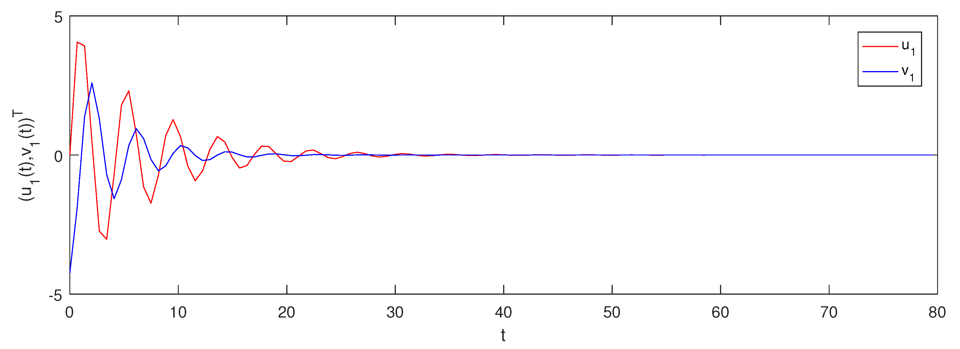
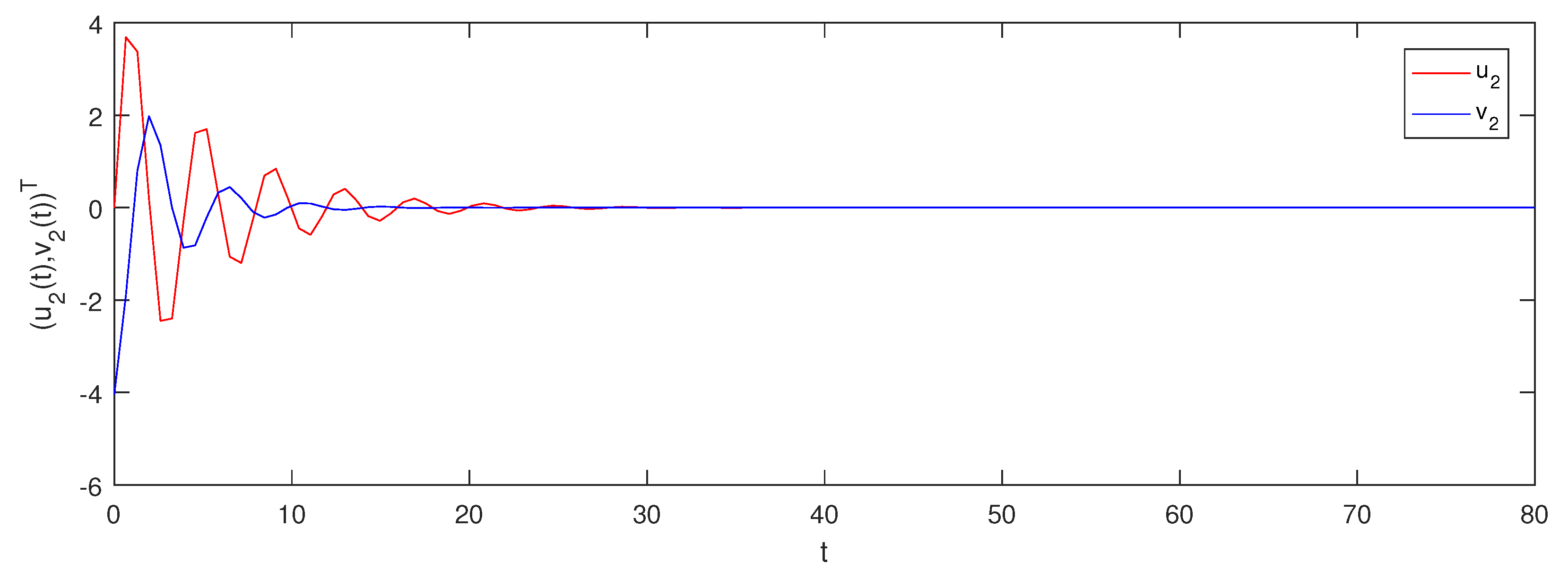
Theorem 2.

Assume that all conditions of Theorem 1 satisfy. Then, the periodic solution of system (3) is globally exponentially stable, if

$$\xi >{\rho }_2,$$

(13)

where

$$\xi =\underset{1\le i\le n}{min}\{a_i\left(t\right),{\alpha }_i\left(t\right)\},{\rho }_2=\underset{1\le i\le n}{max}\left\{\sum _{j=1}^n|b_{ij}{|}_0{m}_j{\chi }_j+\sum _{j=1}^n\sum _{k=1}^n|T_{ikj}{|}_0{l}_k{m}_j{\chi }_j,|D_i{|}_0+{|{\beta }_i|}_{0}c{m}_i\right\}.$$

Proof. 

Using Theorem 1, (3) has a periodic solution $w^{*}\left(t\right)={(u^{*}\left(t\right),v^{*}\left(t\right))}^T$, where $u^{*}(·)={(u_1^{*}(·),u_2^{*}(·),\cdots ,u_n^{*}(·))}^T,$ $v^{*}(·)={(v_1^{*}(·),v_2^{*}(·),\cdots ,v_n^{*}(·))}^T$. Let $w\left(t\right)={(u\left(t\right),v\left(t\right))}^T$ be any solution of (3). Let

$${\tilde{w}}_i\left(t\right)=w_i\left(t\right)-w_i^{*}\left(t\right),{\tilde{u}}_i\left(t\right)=u_i\left(t\right)-u_i^{*}\left(t\right),{\tilde{v}}_i\left(t\right)=v_i\left(t\right)-v_i^{*}\left(t\right),$$

$$g_j\left({\tilde{u}}_j\left(t\right)\right)=f_j({\tilde{u}}_j\left(t\right)+u_j^{*}\left(t\right))-f_j\left(u_j^{*}\left(t\right)\right).$$

Obviously $g_j\left({\tilde{u}}_j\left(t\right)\right)$ satisfies (H₃). System (3) can be rewritten as follows:

$$\begin{array}{cc}\hfill {\tilde{u}}_i^{\prime }\left(t\right)& =-a_i\left(t\right){\tilde{u}}_i\left(t\right)+\sum _{j=1}^n{b}_{ij}\left(t\right)g_j\left({\tilde{u}}_j(t-{\gamma }_j\left(t\right))\right)\hfill \\ \hfill & +\sum _{j=1}^n\sum _{k=1}^n{T}_{ijk}\left(t\right)g_j\left({\tilde{u}}_j(t-{\gamma }_j\left(t\right))\right)g_k\left({\tilde{u}}_k(t-{\gamma }_k\left(t\right))\right)+D_i\left(t\right){\tilde{v}}_i\left(t\right),\hfill \end{array}$$

(14)

$${\tilde{v}}_i^{\prime }\left(t\right)=-{\alpha }_i\left(t\right){\tilde{v}}_i\left(t\right)+{\beta }_i\left(t\right)c{g}_i\left({\tilde{u}}_i\left(t\right)\right).$$

(15)

For $t\ge 0$, using (14) we obtain

$$\begin{array}{cc}\hfill {\tilde{u}}_i\left(t\right)& =e^{-{\int }_0^t{a}_i\left(r\right)dr}{\tilde{u}}_i\left(0\right)+e^{-{\int }_0^t{a}_i\left(r\right)dr}{\int }_0^t(\sum _{j=1}^n{b}_{ij}\left(r\right)g_j\left({\tilde{u}}_j(r-{\gamma }_j\left(r\right))\right)\hfill \\ \hfill & +\sum _{j=1}^n\sum _{k=1}^n{T}_{ijk}\left(r\right)g_j\left({\tilde{u}}_j(r-{\gamma }_j\left(r\right))\right)g_k\left({\tilde{u}}_k(r-{\gamma }_k\left(r\right))\right)+D_i\left(r\right){\tilde{v}}_i\left(r\right))e^{{\int }_0^r{a}_i\left(u\right)du}dr.\hfill \end{array}$$

(16)

Furthermore, for $t\ge 0$, using (15) we obtain

$${\tilde{v}}_i\left(t\right)=e^{-{\int }_0^t{\alpha }_i\left(r\right)dr}{\tilde{v}}_i\left(0\right)+e^{-{\int }_0^t{\alpha }_i\left(r\right)dr}{\int }_0^t\left({\beta }_i\left(r\right)c{g}_i\left({\tilde{u}}_i\left(r\right)\right)\right)e^{{\int }_0^r{\alpha }_i\left(u\right)du}dr.$$

(17)

Using (14), (H₂), and (H₃), we have

$$\begin{array}{cc}\hfill |{\tilde{u}}_i\left(t\right)|& \le e^{-{\int }_0^t{a}_i\left(r\right)dr}[|{\tilde{u}}_i\left(0\right)|+{\int }_0^t(\sum _{j=1}^n|b_{ij}{|}_0{m}_j|{\tilde{u}}_j(r-{\gamma }_j\left(r\right))|\hfill \\ \hfill & +\sum _{j=1}^n\sum _{k=1}^n|T_{ijk}{|}_0{l}_j{m}_k|{\tilde{u}}_k(r-{\gamma }_k\left(r\right))|+|D_i{|}_0|{\tilde{v}}_i\left(r\right)|\left)e^{{\int }_0^r{a}_i\left(u\right)du}dr\right]\hfill \\ \hfill & \le e^{-\xi t}|{\tilde{u}}_i\left(0\right)|+e^{-\xi t}\sum _{j=1}^n|b_{ij}{|}_0{m}_j{\chi }_j{\int }_{-|{\gamma }_j{|}_0}^{t-{\gamma }_j\left(t\right)}|{\tilde{u}}_j\left(r\right)|e^{|a_i{|}_0(r+|{\gamma }_j{|}_0)}dr\hfill \\ \hfill & +e^{-\xi t}\sum _{j=1}^n\sum _{k=1}^n|T_{ikj}{|}_0{l}_k{m}_j{\chi }_j{\int }_{-|{\gamma }_j{|}_0}^{t-{\gamma }_j\left(t\right)}|{\tilde{u}}_j\left(r\right)|e^{|a_i{|}_0(r+|{\gamma }_j{|}_0)}dr\hfill \\ \hfill & +e^{-\xi t}|D_i{|}_0{\int }_0^t|{\tilde{v}}_i\left(r\right)|e^{|a_i{|}_{0}r}dr\hfill \\ \hfill & \le e^{-\xi t}\left[|{\tilde{u}}_i\left(0\right)|+\left(\sum _{j=1}^n|b_{ij}{|}_0{m}_j{\chi }_j{e}^{|a_i{|}_0{|{\gamma }_j|}_0}+\sum _{j=1}^n\sum _{k=1}^n{|T_{ikj}|}_0{l}_k{m}_j{\chi }_j{e}^{|a_i{|}_0{|{\gamma }_j|}_0}\right)\underset{-\tau \le s\le 0}{max}|{\tilde{u}}_j\left(s\right)|\right]\hfill \\ \hfill & +e^{-\xi t}\left(\sum _{j=1}^n|b_{ij}{|}_0{m}_j{\chi }_j+\sum _{j=1}^n\sum _{k=1}^n{|T_{ikj}|}_0{l}_k{m}_j{\chi }_j\right){\int }_0^t|{\tilde{u}}_i\left(r\right)|e^{|a_i{|}_{0}r}dr\hfill \\ \hfill & +e^{-\xi t}|D_i{|}_0{\int }_0^t|{\tilde{v}}_i\left(r\right)|e^{|a_i{|}_{0}r}dr.\hfill \end{array}$$

(18)

From (15) and (H₃), we have

$$\begin{array}{cc}\hfill |{\tilde{v}}_i\left(t\right)|& \le e^{-\xi t}|{\tilde{v}}_i\left(0\right)|+e^{-\xi t}|{\beta }_i{|}_{0}c{m}_i{\int }_0^t|{\tilde{u}}_i\left(r\right)|e^{|a_i{|}_{0}r}dr.\hfill \end{array}$$

(19)

From (18) and (19), we obtain

$$\begin{array}{cc}\hfill \delta \left(t\right)& =\sum _{i=1}^n(|{\tilde{u}}_i\left(t\right)|+|{\tilde{v}}_i\left(t\right)|)\hfill \\ & \le {\rho }_1||\varphi -{\varphi }^{*}||e^{-\xi t}+{\rho }_2{\int }_0^t\delta \left(r\right)e^{\xi (r-t)}dr,\hfill \end{array}$$

where

$${\rho }_1=2+\underset{1\le n}{max}\left(\sum _{j=1}^n|b_{ij}{|}_0{m}_j{\chi }_j{e}^{|a_i{|}_0{|{\gamma }_j|}_0}+\sum _{j=1}^n\sum _{k=1}^n{|T_{ikj}|}_0{l}_k{m}_j{\chi }_j{e}^{|a_i{|}_0{|{\gamma }_j|}_0}\right),$$

${\rho }_2$ is defined by (13). Using Gronwall’s inequality, we obtain

$$\delta \left(t\right)=\sum _{i=1}^n(|{\tilde{u}}_i\left(t\right)|+|{\tilde{v}}_i\left(t\right)|)\le {\rho }_1||\varphi -{\varphi }^{*}||e^{-(\xi -{\rho }_2)t}.$$

Due to Definition 1, there exists a globally exponentially stable periodic solution for system (3). □

Remark 2.

Usually, the Lyapunov–Kravsovskii functional method is the main method for studying the stability of equations, and a large number of stability results are obtained using this method. But constructing a suitable Lyapunov function is very difficult. In this article, we use the basic theory of differential equations and Gronwall’s inequality to obtain the dynamical behaviors of system (3). The method presented in this article is easier to understand and the proof process is not complicated.

5. Example

Consider the following Hebbian-type networks:

$$\begin{array}{cc}\hfill u_1^{\prime }\left(t\right)& =-(12-sint)u_1\left(t\right)+sint{f}_1\left(u_1(1-\frac{1}{2}sint)\right)+sint{f}_2\left(u_2(1-\frac{1}{2}sint)\right)\hfill \\ \hfill & +cost{f}_1\left(u_1(1-\frac{1}{2}sint)\right)f_1\left(u_1(1-\frac{1}{2}sint)\right)+sint{f}_1\left(u_1(1-\frac{1}{2}sint)\right)+sint{f}_2\left(u_2(1-\frac{1}{2}sint)\right)\hfill \\ \hfill & +cost{f}_2\left(u_2(1-\frac{1}{2}sint)\right)f_1\left(u_1(1-\frac{1}{2}sint)\right)+cost{f}_2\left(u_2(1-\frac{1}{2}sint)\right)f_2\left(u_2(1-\frac{1}{2}sint)\right)+(\frac{1}{5}cost)v_1\left(t\right),\hfill \\ \hfill v_1^{\prime }\left(t\right)& =-(10-cost)v_1\left(t\right)+\frac{1}{2}sint{f}_1\left(u_1\left(t\right)\right),\hfill \\ \hfill u_2^{\prime }\left(t\right)& =-(12-sint)u_2\left(t\right)+sint{f}_1\left(u_1(1-\frac{1}{2}sint)\right)+sint{f}_2\left(u_2(1-\frac{1}{2}sint)\right)\hfill \\ \hfill & +cost{f}_1\left(u_1(1-\frac{1}{2}sint)\right)f_1\left(u_1(1-\frac{1}{2}sint)\right)+sint{f}_1\left(u_1(1-\frac{1}{2}sint)\right)dt+sint{f}_2\left(u_2(1-\frac{1}{2}sint)\right)\hfill \\ \hfill & +cost{f}_2\left(u_2(1-\frac{1}{2}sint)\right)f_1\left(u_1(1-\frac{1}{2}sint)\right)+cost{f}_2\left(u_2(1-\frac{1}{2}sint)\right)f_2\left(u_2(1-\frac{1}{2}sint)\right)+(\frac{1}{5}cost)v_2\left(t\right),\hfill \\ \hfill v_2^{\prime }\left(t\right)& =-(10-cost)v_2\left(t\right)+\frac{1}{2}sint{f}_2\left(u_2\left(t\right)\right),\hfill \end{array}$$

(20)

where

$$i,j,k=1,2,a_i\left(t\right)=12-sint,{\alpha }_i\left(t\right)=10-cost,f_1\left(x\right)=f_2\left(x\right)=\frac{1}{10}\tanh x,$$

$${\gamma }_j\left(t\right)=1-\frac{1}{2}sint,I_i\left(t\right)=0,b_{ij}\left(t\right)=sint,D_i\left(t\right)=\frac{1}{5}cost,c=1,$$

$${\beta }_i\left(t\right)=\frac{1}{2}sint,T_{ijk}=cost.$$

After simple calculations, we have

$$l_j=m_j=\frac{1}{10},\tau =\frac{3}{2},{\chi }_j=2,|b_{ij}{|}_0=|T_{ijk}{|}_0=1,|D_i{|}_0=\frac{1}{5},{|{\beta }_i|}_0=\frac{1}{2},$$

$${\nu }_1=\underset{1\le i\le n}{min}\left\{{\overline{a}}_i-\sum _{j=1}^n|{\overline{b}}_{ji}|m_i-\sum _{j=1}^n\sum _{k=1}^n|{\overline{T}}_{kji}|l_j{m}_i-|{\overline{\beta }}_i|c{m}_i\right\}=12,$$

$${\nu }_2=\underset{1\le i\le n}{min}\left\{{\overline{\alpha }}_i-|{\overline{D}}_i|\right\}=10,\xi =\underset{1\le i\le n}{min}\{a_i\left(t\right),{\alpha }_i\left(t\right)\}=9,$$

$${\rho }_2=\underset{1\le i\le n}{max}\left\{\sum _{j=1}^n|b_{ij}{|}_0{m}_j{\chi }_j+\sum _{j=1}^n\sum _{k=1}^n|T_{ikj}{|}_0{l}_k{m}_j{\chi }_j,|D_i{|}_0+{|{\beta }_i|}_{0}c{m}_i\right\}=0.51.$$

We obtain ${\nu }_1,{\nu }_2>0$ and $\xi >{\rho }_2$. From selections of $f_1\left(x\right)$ and $f_2\left(x\right)$, it is obvious that there exists a periodic solution for system (20) ${(0,0)}^T$. Furthermore, using the above calculations, we confirm that all conditions of Theorem 1 and Theorem 2 satisfy. Hence, there exists a globally asymptotically periodic solution for system (20) ${(0,0)}^T$. Figure 1 and Figure 2 show the evolution of the solution of system (20).

6. Conclusions and Discussions

We study a class of Hebbian-type networks with variable lags. More precisely, we obtain some criteria for the existence of a periodic solution. Also, we examine the globally exponential stability analysis of system (3). Finally, we provided an example to show the analytical results. We can further investigate the dynamic behavior of system (3) under different environmental interference factors. One aspect future research is the stochastic Hebbian-type networks.

References

1. Gopalsamy, K. Learning dynamics in second order networks. Nonlinear Anal. Real World Appl. 2007, 8, 688–698. [Google Scholar] [CrossRef]
2. Amari, S. Competitive and cooperative aspects in dynamics of neural excitation and self-organization. In Competition and Cooperation in Neural Nets; Lecture Notes in Biomathematics; Springer: Berlin/Heidelberg, Germany, 1982. [Google Scholar]
3. Amari, S. Mathematical theory of neural learning. New Gener. Comput. 1991, 8, 281–294. [Google Scholar] [CrossRef]
4. Gonzalez, M.; Basin, M.; Vargas, E. Discrete-time high-order neural network identifier trained with high-order sliding mode observer and unscented Kalman filter. Neurocomputing 2021, 424, 172–178. [Google Scholar] [CrossRef]
5. Huang, C.; Cao, J. Bifurcations due to different delays of high-order fractional neural networks. Int. J. Biomath. 2022, 15, 2150075. [Google Scholar] [CrossRef]
6. Liu, D.; Liu, Z.; Zhang, Y.; Chen, C. Neural network-based smooth fixed-time cooperative control of high-Order multi-agent systems with time-varying failures. J. Frankl. Inst. 2022, 359, 152–177. [Google Scholar] [CrossRef]
7. Huang, Z.; Raffoul, Y.; Cheng, C. Scale-limited activating sets and multiperiodicity for threshold-linear networks on time scales. IEEE Trans. Cybern. 2014, 44, 488–499. [Google Scholar] [CrossRef] [PubMed]
8. Cao, J.; Liang, J.; Lam, J. Exponential stability of high order bidirectional associative memory neural networks with time delays. Physica D 2004, 199, 425–436. [Google Scholar] [CrossRef]
9. Kosmatopoulos, E.; Polycarpou, M.; Christodoulou, M.; Ioannou, P. High order neural network structures for identification of dynamical systems. IEEE Trans. Neural Netw. 1995, 6, 422–431. [Google Scholar] [CrossRef]
10. Liu, Y.; Wang, Z.; Liu, X. An LMI approach to stability analysis of stochastic high-order Markovian jumping neural networks with mixed time delays. Nonlinear Anal. Hybrid Syst. 2008, 2, 110–120. [Google Scholar] [CrossRef]
11. Xing, J.; Peng, C.; Cao, Z. Event-triggered adaptive fuzzy tracking control for high-order stochastic nonlinear systems. J. Frankl. Inst. 2022, 359, 6893–6914. [Google Scholar] [CrossRef]
12. Wu, W.; Yang, L.; Ren, Y. Periodic solutions for stochastic Cohen—CGrossberg neural networks with time-varying delays. Int. J. Nonlinear Sci. Numer. Simul. 2021, 22, 13–21. [Google Scholar] [CrossRef]
13. Zhang, Z.; Liu, K. Existence and global exponential stability of a periodic solution to interval general bidirectional associative memory (BAM) neural networks with multiple delays on time scales. Neural Netw. 2011, 24, 427–439. [Google Scholar] [CrossRef] [PubMed]
14. Luo, D.; Jiang, Q.; Wang, Q. Anti-periodic solutions on Clifford-valued high-order Hopfield neural networks with multi-proportional delays. Neurocomputing 2022, 472, 1–11. [Google Scholar] [CrossRef]
15. Li, Y.; Xiang, J. Existence and global exponential stability of almost periodic solution for quaternion-valued high-order Hopfield neural networks with delays via a direct method. Math. Methods Appl. Sci. 2020, 43, 6165–6180. [Google Scholar] [CrossRef]
16. Guo, X.; Huang, C.; Cao, J. Nonnegative periodicity on high-order proportional delayed cellular neural networks involving D operator. AIMS Math. 2021, 6, 2228–2243. [Google Scholar] [CrossRef]
17. Cao, Q.; Guo, X. Anti-periodic dynamics on high-order inertial Hopfield neural networks involving time-varying delays. AIMS Math. 2020, 5, 5402–5421. [Google Scholar] [CrossRef]
18. Gao, J.; Dai, L. Anti-periodic synchronization of quaternion-valued high-order Hopfield neural networks with delays. AIMS Math. 2022, 7, 14051–14075. [Google Scholar] [CrossRef]
19. Huang, C.; Liu, B.; Qian, C.; Cao, J. Stability on positive pseudo almost periodic solutions of HPDCNNs incorporating D operator. Math. Comput. Simul. 2021, 190, 1150–1163. [Google Scholar] [CrossRef]
20. Duan, L.; Huang, L.; Guo, Z.; Fang, X. Periodic attractor for reaction—Cdiffusion high-order hopfield neural networks with time-varying delays. Comput. Math. Appl. 2017, 73, 233–245. [Google Scholar] [CrossRef]
21. Gaines, R.; Mawhin, J. Coincidence Degree and Nonlinear Differential Equations; Springer: Berlin/Heidelberg, Germany, 1977. [Google Scholar]
Figure 1. Evolution for the solution ( u 1 ( t ) , v 1 ( t ) ) T of system (20).
Symmetry 15 01985 g001
Figure 2. Evolution for the solution ( u 2 ( t ) , v 2 ( t ) ) T of system (20).
Symmetry 15 01985 g002
Disclaimer/Publisher’s Note: The statements, opinions and data contained in all publications are solely those of the individual author(s) and contributor(s) and not of MDPI and/or the editor(s). MDPI and/or the editor(s) disclaim responsibility for any injury to people or property resulting from any ideas, methods, instructions or products referred to in the content.