Monetary Datum Fractal Analysis Using the Time Series Theory

Abstract

The paper will allow the interpretation of exchange rate fluctuations for several international currencies, the EUR—European currency and the CHF—Swiss Franc, respectively. The fractal dimension versus box-counting dimension, together with the fractal dimension versus log scale for CHF and EUR, respectively, are thoroughly presented. The exchange rate time series for CHF and EUR during March–June 2022 were also analyzed. The Hurst exponent H was numerically evaluated. By the application of directional symmetry (DS) statistics, the model efficiency in predicting the direction modification of time series has been verified. Ultimately, the prognosis of EUR-RON and CHF-RON exchange rates of the time series fluctuations for the last months (August–December) of the year 2022 was performed.

1. Introduction

Fractal analysis is a contemporaneous modern procedure that applies nonorthodox mathematics to geometrical shapes and infringes the alignment to classical Euclidean convictions; it is, in fact, exclusively based on non-Euclidean geometry principles.

However, the so-called popular fractals are not inevitably substantial shapes—but, on the contrary, they may be spatial or temporal structures. Universally, fractals are a category of infinitely dialed, transcribed, and reiterated geometrical models [1].

Therein, it is significant that mathematical fractals are ideal abstract entities, but the fractal analysis representations, such as digital pictures restricted by device display resolution, are normally not authentic fractals in a strict sense [2].

The fractal dimension represents a real number situated between the topological dimension of the object and the dimension of the space in which it is defined [3]. The fact that the size of an object can be any real positive number (so not necessarily an integer number) is at least disturbing in classical thinking. However, an exact definition of the fractal dimension has not yet been found, much less a general formula for calculating this dimension, although it is generally estimated by calculating the logarithmic ratio of some properties at different scales. Finally, historically speaking, in the year of Grace 1975, Mandelbrot coined the term “fractal” to refer to an object whose Hausdorff–Besicovitch dimension is larger than its topological dimension.

Throughout the last decades, the presence and exploitation of financial time series and the interpretation of existing financial data expressed in time series databases were of prominent importance in investigating, retaining, and depicting underlying cases implicated by these data. Today, without being a fashion, this concern has a remarkable purpose in backing and assisting the traditional methods utilized in financial banking domains. In addition, the exploitation manner of these temporal archives turned out to be very efficient and completely advantageous, which turned them into the most used means of applied financial research.

The financial market is an important slice of a piazza system, which is produced by money supply in contrast with both money demand and capital offer. There are a minimum of four financial market distinct partitions, such as commodity market, stock market, exchange market, and bond market. The financial market is an affairs piazza with loans, credits, commodities, bonds, currency, and shares. The price index is considered as an essential information in open financial markets. Among the prices recognized in the market, we can list the most famous ones: bond price, commodity price, price of share, and currency price. To obtain a mathematically correct time series, the current price will be surveilled in a precise time frequency, and the classical time series will be generated. These temporary data suites built according to the recipe above, as well as time series founded on price index or time series that report prices and their temporal comportment, are named financial time series. All these techniques and methods presented here (in continuation of the paper) have been successfully applied to the analysis of financial data and have been used in issuing exchange rate forecasts for the end of this year. The CHF and EUR exchange rates during March–June 2022 were analyzed because we opted for the temporal series with the smallest oscillations of 2022 and to have a determined number of time elements (number of days), as the theory says.

As stipulated in the theory of the analysis of the fluctuations of a temporal series over time, a maximum time horizon was chosen, namely the last months (August–December) of the year 2022, which is the maximum period of the temporal series considered a very short series (N ≤ 128) type. The purpose of this study is to analyze the exchange rate of time series for CHF and EUR during March–June 2022 using the fractal analysis (fractal dimension and Hurst exponent). In this regard, the model efficiency will be checked in predicting the direction of time series evolution by applying directional symmetry (ds) statistics. Finally, a forecast of EUR-RON and CHF-RON, a rate of the time series fluctuations for the last months (August–December) of the year 2022, will be provided.

In the literature, the methods of fractal analysis are rarely used, respectively, the calculation of the values of the fractal dimension and the Hurst exponent, as well as the technique of prediction of time series evolution by applying directional system (DS) statistics, due to the management difficulties of higher mathematics. This article is among the few that address these methods and use them in the numerical evaluation of the Hurst exponent, but also to obtain successful forecasts on the evolution of EUR-RON and CHF-RON exchange rates in the case of the time series fluctuation procedure. In this way, the most constant currency at foreign exchange can be established, so one can know the currency in which it can be invested during the period supported by the prediction.

This article has five distinct chapters, along with a bibliography that summarizes the representative papers in the field. These are entitled as follows: the first chapter is 1. Introduction, the second chapter refers to 2. Materials and Methods, the third chapter deals with the presentation of 3. Results, the fourth chapter is consecrated to 4. Discussion, and the last chapter is dedicated to 5. Conclusions of this paper.

2. Materials and Methods

The databases used were provided by the values of the RON-EUR exchange rate and RON-CHF exchange rate between 1 March 2022 and 31 July 2022, respectively, from official data of the RNB (Romanian National Bank) during the year 2022 [3]. The software that has been utilized to assist in the realization of our analysis was developed by the authors.

2.1. Fractal Dimension Calculation Formulas

It starts from the fact that an object that has dimension D, composed of several elements similar to it, can be divided into “nD” elements “n” times smaller than the original one. We can now calculate this dimension with the approximate formula:

$$D=\underset{n\to \infty }{\lim }\frac{log\left(Component Number\right)}{ log\left(n\right)}$$

(1)

Because the necessary condition for the validity of this formula is the similarity between the object in discussion and its constituent parts, this approximation of the fractal dimension is also called the self-similarity dimension [1]. In other words, the ratio between the logarithm of the number of segments “n” in which the measured structure can be divided and the measurement scale “s” is called the dimension of self-similarity:

$$D=\frac{log\left(n\left(s\right)\right)}{log\left(s\right)}$$

(2)

The fractal dimension of an object describes how it occupies the space provided and, last but not least, how it can be measured in a quantitative manner. It was expressed by a rational number in the last resort. It can be calculated using the Hausdorff dimension below:

$$N\left(s\right)=f\left(d\right)\ast s^D$$

(3)

where the established notations N(s) = number of cubes, d = number of d-dimensional cubes needed to cover the total space, s = the length of the side of the cube, and D = the fractal dimension of the object. For the coefficient f(d) = 1, the fractal dimension of the object D = logN/logs [2].

Following the aprofonded study and further development of Hausdorff’s avant-garde works, Besicovitch stated that nonuniform shapes might have correct fractional dimensions. Thus, curves such as those of Sierpinski or Koch would fall between normal dimensions and, in this way, could explain their strange mathematical behavior. The Hausdorff–Besicovitch dimension was calculated accurately on measurements made based on simple geometric approximations of this given nonsmooth curve. The Hausdorff–Besicovitch fractal dimension D of a mathematical object [4] in a metric space is determined with the following expression:

$$D=\underset{h\to 0}{\lim }\frac{logN\left(h\right)}{ log\left(\frac{1}{h}\right)}=-\underset{h\to 0}{\lim }\frac{logN\left(h\right)}{logh}$$

(4)

where N(h) is the total disks number of size h needed to completely cover the geometrical object.

Nowadays, a growing number of scientists tend to take fractal dimension (calculating Hausdorff dimension, in fact) [5] as the standard measure of self-similarity and complexity degree in non-Euclidian geometry.

Therefore, to accurately compute the Hausdorff dimension of a fractal object in a direct manner will be especially fastidious because its measure does not constantly have a particular value but fluctuates within a certain range, so many savants promote an additional gauge-like called the box-counting dimension, to do this calculus feasible, evidently. More precisely, the box-counting dimension assumes boxes as the measure; thus, it can be widely used and then recognized by numerous researchers working on investigations of fractal objects because it is easy to calculate and it has the whole definition identical to the Hausdorff dimension definition, in extremely numerous situations [6].

To compute the box-counting dimension, the examined figures must be divided into quadrates, as boxes with facet lengths of ε, and to cover entirely the fractal figure, only such cassettes are used. These boxes covering the initial geometrical object will be considered as being N in total number.

Almost as in the event that total curve lengthiness suffers essential changes relating to each ruler dimension inserted previously, the total cassette number also differs as the magnitude of each box is modified. The notional box-counting dimension is the report limit between log(N) and log(1/ε) in the case in which ε tends to zero, as in the following formula:

$$D_{box}=\underset{\epsilon \to 0}{\lim }\frac{logN\left(\epsilon \right)}{ log\left(\frac{1}{\epsilon }\right)}=-\underset{\epsilon \to 0}{\lim }\frac{logN\left(\epsilon \right)}{log\epsilon }$$

(5)

According to the procedure of cassette numbering and its consideration as a universal generic measure, the box-counting iterative method [7] may be admitted as valuable both for factitious and genuine fractals, regardless of their complexity.

2.2. Time Series Theory

The time series graph illustrates values of the information measured at successive time intervals (possibly equal). This is a two-dimensional graphical representation increment/measure of the time on the abscissa axis (ox axis), following that on the ordinate axis, the values of the measured variable are represented in representative units of measurement [7,8,9]. Thus, when the respective values are represented in chronological order and a straight line, a system of associated peaks and valleys falls connects the adjacent points. Depending on the intended purpose, a simple visual inspection can most easily highlight the study intervals in which we can analyze the monotony of the trend, the correlation, and the dispersion of the points so we can identify a certain trend or we can observe a local extreme point.

We will now introduce the economic time series and the financial time series and explain the difference between them. Their formal definitions can be read in the introduction. In contrast with the other economic time series listed above, the financial time series possesses a few defining properties and forms specified via the financial piazza microstructure. The fundamental attribute of the financial time series is a lofty frequency for its individual reference values. This fact leads to the escalation of the pressure of nonsystematic factors to the time series (chronological) vitality, the result being relatively large volatility, which can currently modify into time. In the opposite sense, the temporal systematic circumstances generate a tendency and cyclic partition of the time series. At the same time, practically, the seasonal side of time series exhibits commonly no notable role [5].

2.2.1. Simple Formal Definition of a Time Series

First, when observing the time series $\left\{x_t\right\}$ habitually, we suppose that $\left\{x_t\right\}$ is an achievement of an aleatory process $\left\{X_t\right\}$. Next, we will introduce the mathematical formalization of this notion here [10]. The aleatory process $\left\{X_t;t\in \mathbb{Z}\right\}$ (wherein $\mathbb{Z}$ indicates the integer numbers) is defined on the likelihood space $\{\mathsf{\Omega },ℱ,P\}$. An explanation of what these constraints signify in continuation is as follows:

(i)

$\mathsf{\Omega }$ is a set with all possible consequences. Assume that $\omega \in \mathsf{\Omega }$, but that $\left\{X_t\left(\omega \right)\right\}$ is one achievement of the aleatory process. Respective to any given $\omega$, $\left\{X_t\left(\omega \right)\right\}$ is not aleatory. In a standard time series, we will habitually suppose that we notice $x_t\in X_t\left(\omega \right)$(for some $\omega$) is a representative realization. Moreover, ${\omega }^{*}\in \mathsf{\Omega },X_t\left({\omega }^{*}\right)$ will be dissimilar for any other, but its global characteristics will be similar in all aspects [11].

(ii)

$ℱ$ algebra is acquainted as a sigma-algebra type. It is a set/crowd of $\mathsf{\Omega }$ subcrowds (although it is not automatically the set of all subsets because it can be too big). Nevertheless, it is constituted of all sets for which a likelihood can be attributed. The truth is that if $A\in ℱ$, likelihood is attributed to the crowd $A$.

(iii)

$P$ is the likelihood measure across the one named sigma-algebra $ℱ$. For every crowd $A\in ℱ$ we can delineate a likelihood $\left(A\right)$. However, it can be said that there are bizarre cases where there is a $\mathsf{\Omega }$ subcrowd that does not belong to the sigma-algebra $ℱ$, where $P\left(A\right)$ cannot be delineated. These crowds are called crowds with nonmeasurable structures, respectively, unmeasurable sets.

Note: the simple definition provided is one of the most general known.

By and large, the time series has a simple formula $X\left(t\right)=\beta x\left(t\right)+\epsilon \left(t\right)$, where $X\left(t\right)=\left\{X_t:t=0,\pm 1,\pm 2,\dots \right\}$ is a certain succession, indexed by the small letter t, the time representative subscript. The actual formula is a mathematical connection of an observable signal-message succession $x\left(t\right)=\left\{x_t\right\}$ and a succession from unobservable white-noise signal-message $\epsilon \left(t\right)=\left\{{\epsilon }_t\right\}$ of several similarly distributed aleatory variables.

2.2.2. Directional Symmetry (DS) Concept of Time Series

In statistical behavior analysis from the time series theory, directional symmetry notion is a well-defined concept. More precisely, this is the statistical estimate of the model performance in prevising the amendment in the direction of evolution, the positive or negative sense carried out, compared to the average trajectory, respectively, the behavior change in the given time series, from a chosen time period to the following period [12]. Having within sight a certain time series $\left\{x_t\right\}$ for t, with given values $t_i$ at times i = 1, …, n and a pattern that achieves forecast for those values ${\widehat{t}}_i$ (t ^ i), then the statistical DS (directional symmetry) is determined by the next formula:

$$DS\left(t,\widehat{t}\right)=\frac{100}{n-1}{{\displaystyle \sum }}_{i=2}^n{d}_i \mathrm{for} d_i=\{\begin{array}{c}1, if \left(t_i-t_{i-1}\right)\left({\widehat{t}}_i-{\widehat{t}}_{i-1}\right)>0\\ 0, otherwise.\end{array}$$

(6)

It is only the variable d_i (right member), which can be 1 if $\left(t_i-t_{i-1}\right)\left({\widehat{t}}_i-{\widehat{t}}_{i-1}\right)>0$, where a certain time series {x_t} is calculated for t, with given values t_i at times i = 1,…,n and a time series pattern that achieves forecast for those values ${\widehat{t}}_i$ (t^i), different from t_i. The function defined by Equation (6) is only a function of t (for t_i values) in the left member of the equality, which represents the same thing in the writing “t^i”, which is used only to distinguish the values of t between them, which lead to two different, distinct time series functions.

The statistical DS offers the percentage of appearances in which the trace of the change in value from one period to the following time period is identical for the two-time series, respectively, the actual time series and the prevised time series. The DS statistic gives a size of the model efficiency in predicting the value direction modification. The case DS = 100% would look like a pattern that predicts to perfection the modified direction of a time series from one period to the following time period.

2.2.3. Hurst Exponent

Firstly, Hurst conceived a resized interval analysis to determine the dimension of a reservoir proposed for construction located on the Nile River [13]. For rough calculation of the future reservoir volume, Hurst utilized long-term records of annual liquid deliverances, S. The average deliverance $E_{m,k}\zeta$ on the period of m(k − 1) + 1 to mk years is calculated by the following formula:

$$E_{m,k}\zeta =\frac{1}{m{{\displaystyle \sum }}_{i=m\left(k-1\right)+1}^{mk}\zeta \left(i\right)}, k=1,\dots ,a$$

(7)

where the symbols under discussion have the following signification: n is the number of years/days, m is the length of interval of years/days, a is the number of intervals, $am~n$, and $\xi \left(i\right)$ is the annual River deliverance, with $i=1,\dots ,n$.

The $S_{m,k}$ (standard deviation) of $\xi \left(i\right)$ for the time interval between m(k − 1) + 1 and mk is designated by the following formula:

$$S_{m,k}=\frac{1}{\left(m-1\right)\left\{{{\displaystyle \sum }}_{i=m\left(k-1\right)+1}^{mk}{\left(\xi \left(i\right)-\xi E_{m,k}\right)}^2\right\}}$$

(8)

The $S_m$ (mean standard deviation) of $\xi$ for length lapse m is the average of $S_{m,k}$.

The $\xi \left(i\right)$ called now discharges, were utilized to obtain the capitalized deviations $X_m\left(j\right)$ of the average unloading/discharge $E_{m,k}\zeta$ for everyday j among $m\left(k-1\right)+1$ and $mk$.

$$X_m\left(j\right)={{\displaystyle \sum }}_{i=m\left(k-1\right)+1}^j\left(\xi \left(i\right)-\xi E_{m,k}\right), j=m\left(k-1\right)+1,\dots ,mk$$

(9)

We have $X_m\left(mk\right)=0$ in this context.

The deviation interval $R_{m,k}$ is the $X_m\left(j\right)$ for the time period between m(k − 1) + 1 and mk. It is found with the following formula:

$$R_{m,k}=ma{x}_{j=m\left(k-1\right)+1,mk}{X}_m\left(j\right)-mi{n}_{j=m\left(k-1\right)+1,mk}{X}_m\left(j\right)$$

(10)

The calculated mean $R_m$ across the defined intervals is the tank (reservoir) average capacity, which must be held to never flood, in a time period of m days. The resized interval for a length time period m is the nondimensional quantity $R_m$/$S_m$. The average $R_m$ is adjusted for the mean standard deviation S_m [13].

The Hurst Exponent H is numerically evaluated by adjustment of the power-law to the experimental data:

$$E\left[\frac{R\left(n\right)}{S\left(n\right)}\right]=\underset{n\to \infty }{\lim }C{n}^H$$

(11)

where $E\left[x\right]$ is equal to the expected value, C is a multiplicative constant, and n is the observation time aperture, respectively, data point (days, years, etc.) number in a time series.

In the case of self-similar (or fractal) time series, H is immediately connected to the fractal dimension, D. More precisely, D = 2 − H, with 1 < D < 2. The Hurst exponent values vary between 0 and 1, with higher values suggesting a soft/delicate trend, less volatility, and, finally, less rugosity. For H = 0.5, the Hurst exponent relates to an entirely random system, and for H = 1 to an entirely deterministic system. Natural activities such as rivers’ excess releases of water, multiannual temperature values, and the rings that determine the age of trees hold the Hurst exponents around 0.72.

Note: The Hurst exponent is only one scalar value that recommends the fact that if a time series is purely random, it has a tendency or, rather, returns by itself. Therefore, both momentum and a reversal strategy of average can be validated.

3. Results

3.1. Fractal Dimension

A fractal analysis was performed, more precisely, the evaluation of the fractal dimension of the exchange rate for EUR and CHF, calculated by direct method (in the first case) and box-counting algorithm (in the second case). There was also a graphical correlation of the two methods used, as well as a representation of the value of the fractal dimension as a function of log scale, in the range between −2.0 and 0.0. For both currencies, the value of the fractal dimension is strictly less than two, which is the limit of the classical geometric measure of the two-dimensional space, i.e., of the real plane (R²).

In Figure 1 and Figure 2, the fractal dimension versus box-counting dimension for CHF and the fractal dimension versus log scale for CHF, respectively, are presented.

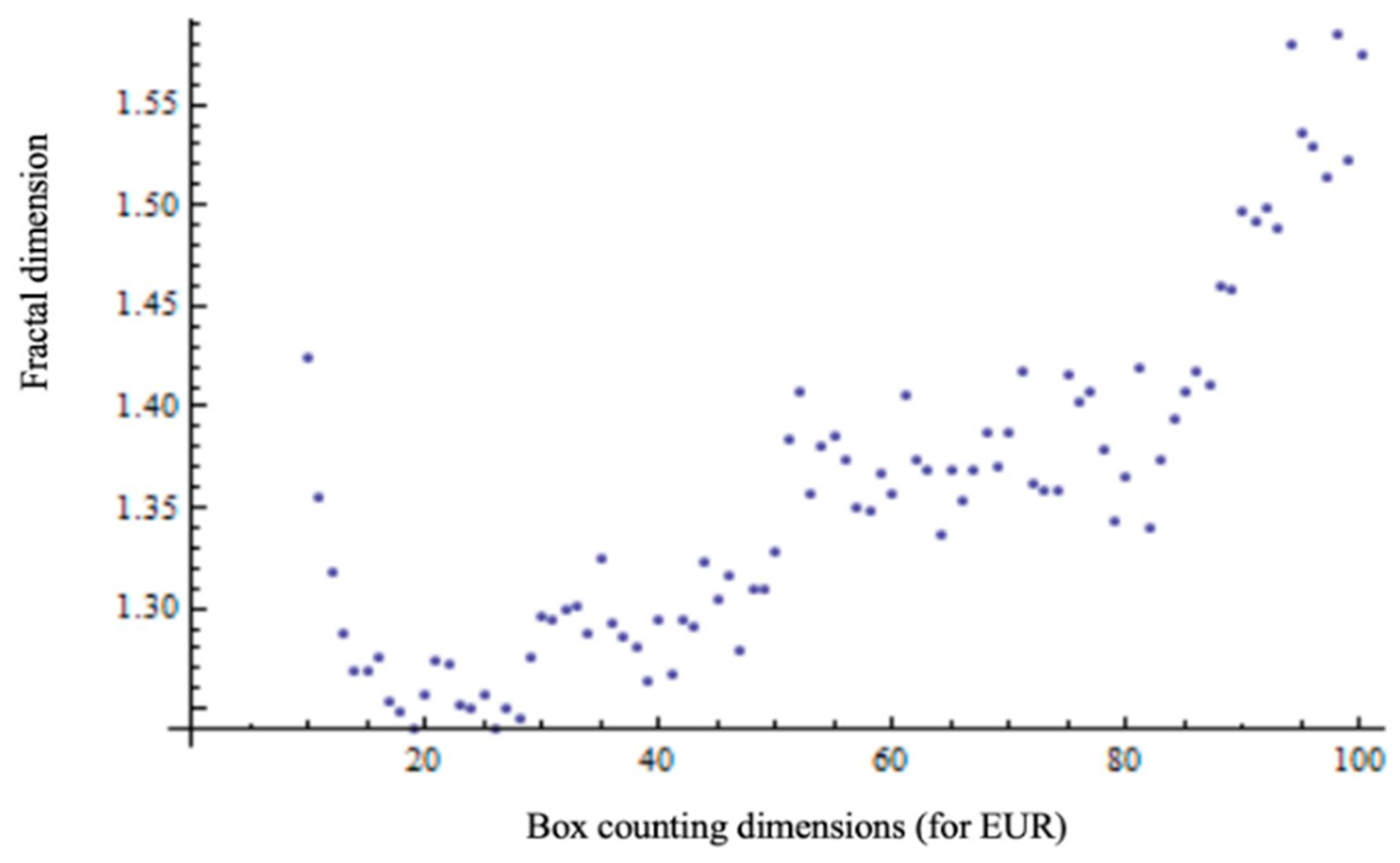
In Figure 3 and Figure 4, the fractal dimension versus box-counting dimension for EUR and the fractal dimension versus log scale for EUR, respectively, are presented.

We note a difference (sometimes significant) between the classical fractal dimension and box-counting dimension, both for CHF, in Figure 1 and for EUR, in Figure 3. In the case of identical evaluation values, the points had to be arranged on the first bisector of the quadrant in which they were represented. However, it is verified that the value of the maximum fractal dimension (around 1.6 for both currencies) is strictly less than 2.

3.2. Time Series Analysis

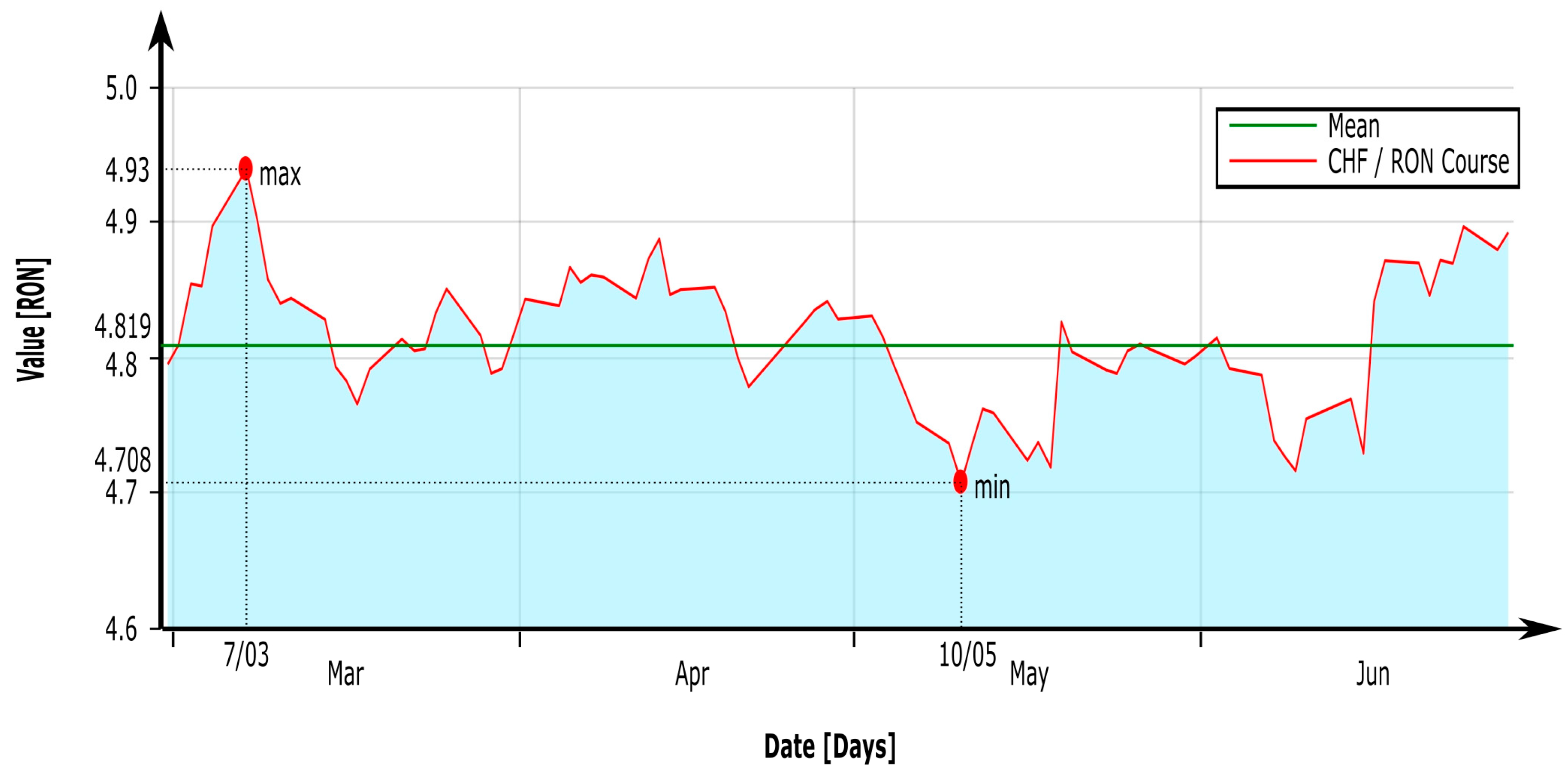
The figures below show graphically the values of the RON-EUR exchange rate and RON-CHF exchange rate between 1 March 2022 and 31 July 2022, respectively, from official data of the RNB (Romanian National Bank) during the year 2022. Through a detailed visual analysis, made carefully, the following characteristics can be observed.

Figure 5 shows the exchange rate for EUR-RON during March–June 2022. A steep slope at the beginning of the year with the highest value of the entire period, followed by a tendency of mediation in sawtooth (see solid red line), is observed. There is a significant decrease in April (11 April 2022) when the minimum value of the transaction for the entire period considered is reached. Regarding the extreme values, we can easily find the minimum value (min = 4.9409) on the date 11 April 2022, followed by the maximum value (max = 4.9490) on the date 8 March 2022. The average value of transactions for the total time is 4.9449.

In Figure 6, the exchange rate for CHF-RON during March–June 2022 is presented. A steep slope at the beginning of the year with the highest value of the entire period, followed by a tendency of mediation in sawtooth (see solid red line), is observed. Regarding the extreme values, we can easily find the minimum value (min = 4.7080) on the date of 10 May 2022, followed by the maximum value (max = 4.9300) on the date of 7 March 2022. The average value of transactions for the total time is 4.8190.

The same time series technique used in analyzing the impact of exchange rates on the stock market was also used by the authors in a materials physics paper [14].

3.3. Hurst Exponent Evaluation

In the box-counting methods, the maximum box dimension is equal to the series half-length for series considered very short time series (N ≤ 128). The number of days N from the 4 months taken into account (March, April, May, and June) is 122 in total. So, the number of points on the abscissa of the two-time series is N = 122.

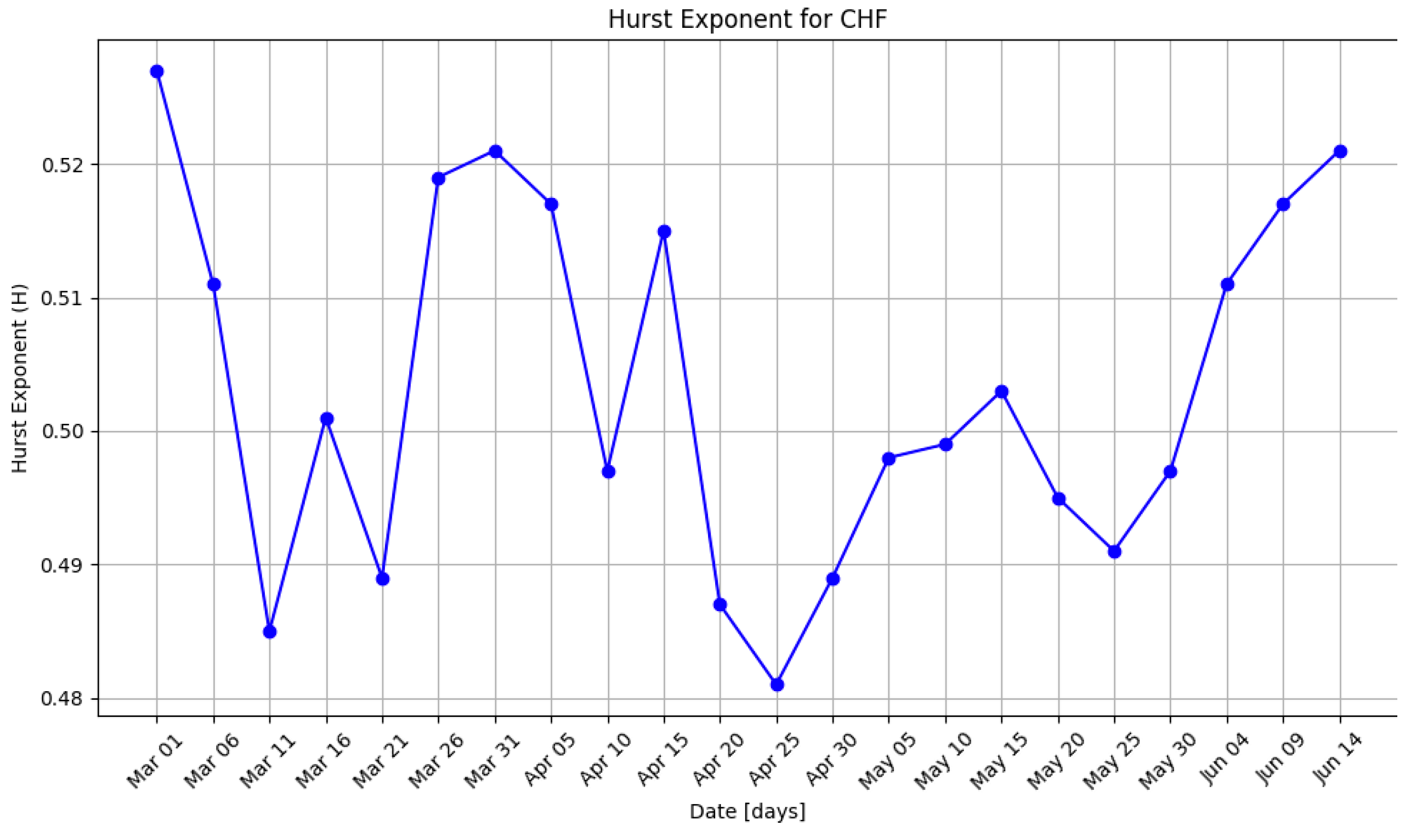
Figure 7 and Figure 8 present the Hurst exponent every five days once taken into consideration, utilizing the 122/5 = 22 as distinct values for those from the new time series chosen. As it is presented in the figure, the Hurst exponent reaches values particularly below 0.5, depending on the fluctuation of the exchange rate. However, there is a significant increase in Hurst’s values in several time windows, which indicates a persistent character of time series. During the period of excessive calmness, the time series manifested an evident antipersistent character. Figure 7 and Figure 8 present the Hurst Exponent, for EUR and for CHF, every five days once taken into consideration.

In Figure 7, the Hurst Exponent for EUR is included between the values 0.477 and 0.539. In Figure 8, the Hurst Exponent for CHF is included between the values 0.481 and 0.527.

The Hurst exponent has 8 H values less than 0.5 and 14 H values greater than 0.5 for the EUR currency (Figure 7), while for the CHF currency, it has 12 H values less than 0.5 and 12 H values greater than 0.5 (Figure 8). Thus, we have distinct parts of the original series with different typologies and not a single typology for the entire series (Figure 5 and Figure 6).

The Hurst exponent H and the fractal dimension D of the same fractal object are linearly connected by the expression D = 2 − H where 0 ≤ H ≤ 1 and 1 ≤ D ≤ 2. Let us now calculate the fractal dimension according to the Hurst exponent experimentally obtained for the exchange rates of the two currencies, D₁ for EUR and D₂ for CHF, respectively. Figure 9 and Figure 10 present the fractal dimension, D₁ for EUR and D₂ for CHF, every five days once taken into consideration.

In Figure 9, the fractal dimension calculated with the formula D₁ = 2 − HE for EUR is included between the values 1.461 and 1.523. In Figure 10, the fractal dimension calculated with the formula D₂ = 2 − HE for CHF is included between the values 1.473 and 1.5519.

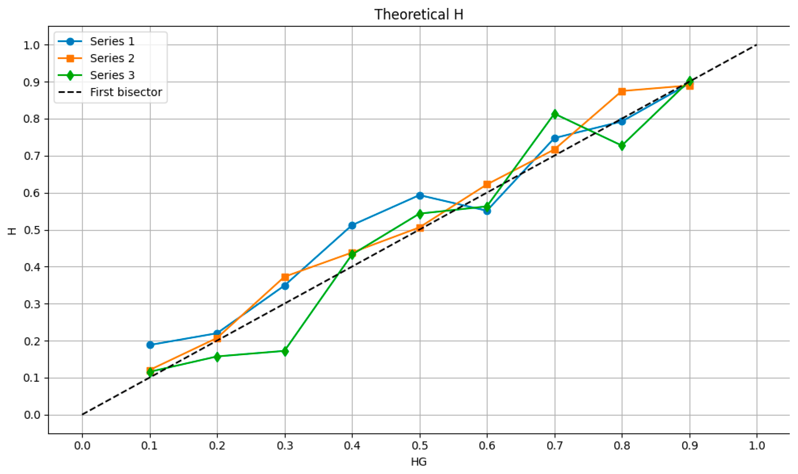
In Figure 11, the Hurst exponents for EUR and CHF are represented on the same graph, both the theoretical ones on one axis and the experimental ones, calculated from the respective series on the other axis. On the abscissa (Ox axis) is HG, the theoretical value of the Hurst exponent, and on the ordinate (Oy axis) is represented H, the estimated value of the Hurst exponent.

Figure 11 shows three representative curves, one for EUR, series 1 in blue color, and another for CHF, series 2 in red color. The third curve, named series 3, green in color, represents the Hurst exponent calculated with the formula H = 2 − D, i.e., equal to the difference between the value two and the fractal dimension D found with the box-counting algorithm.

Equations (4) and (5) were used for Figure 1 and Figure 3, and Equation (2) (for the oy axis), (4), and (5) (for the ox axis) for Figure 2 and Figure 4. Equations (9)–(11) were used in performing the time series analysis regarding the evaluation of the Hurst exponent. Figure 7, Figure 8, Figure 9, Figure 10 and Figure 11 were made with personal software programs for processing the results and raising the adjacent graphs. The software programs that have been utilized to assist the time series analysis realization were developed by the authors and were also used in their own papers present in the bibliography [5,6,10,15].

3.4. Symmetry in Price Formation

Factual analysis utilizes historical former prices to portend future price shifting, whereas basic analysis, by contrast, utilizes gain future estimations to find the correct price for any determinate time. On this occasion, the manner in which the increase in support degree, either at an unstable or stable level, in the price constitution determines symmetries will be described [16].

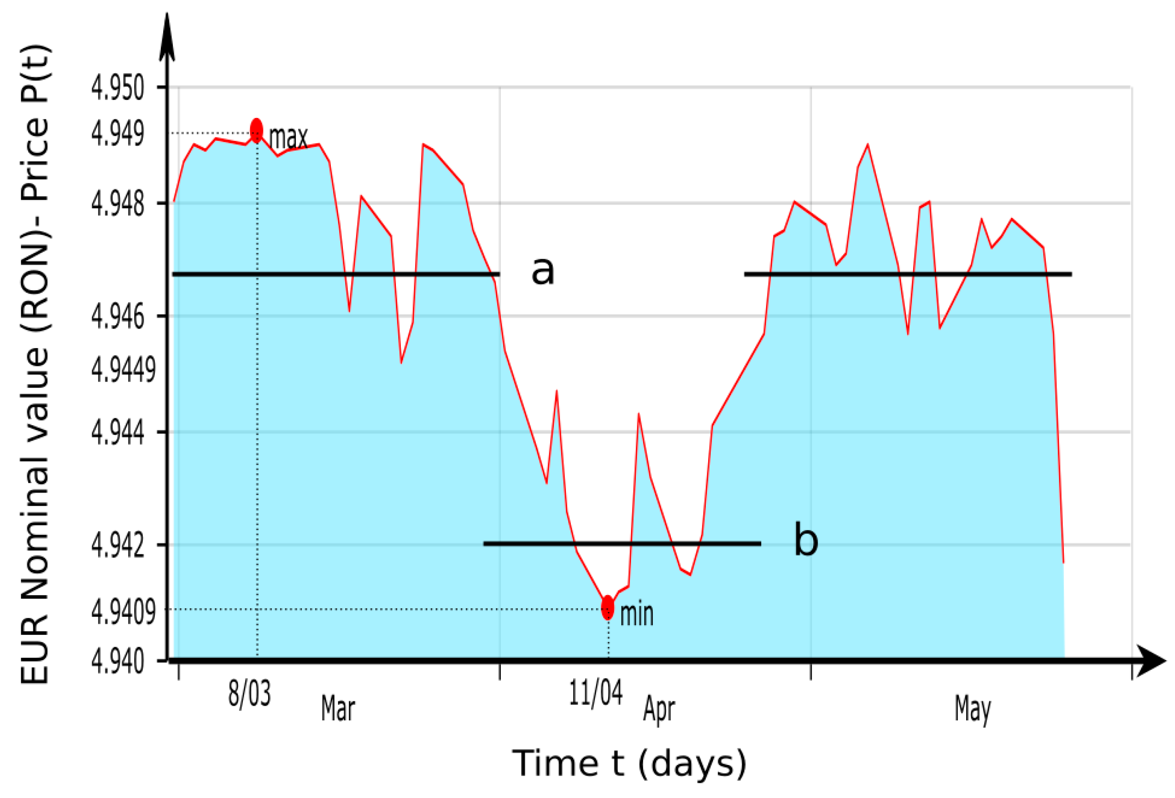
Figure 12 represents the symmetry of one steady and one unsteady supporting level for the price considered as the nominal value of EUR, in RON, every day, basically the nominal value of the EUR currency, every day in the interval months of March, April, and May approximately, monitored.

It can be stated that in terms of symmetry, especially regarding the setting of the price in the market, symmetry breaking occurs from an unsteady supporting level to a steady supporting level, with the highest probability. For instance, it can befall the price constitution on a financial market still considered stable to manifest through amongst required supporting levels; see the diagram from Figure 12 as an example. This chart represents a capture (a cropped portion) from a time series of prices in a well-defined period of time, respectively, an illustration of daily price variations and linear supporting levels.

The comprehension of when those symmetries are destroyed will be driven by well-defined cases for conducting the best possibilities of price arbitrage.

The symmetry destruction from an unstable degree level to a stable degree level can be carried out easily. Occasionally, it could befall that the price constitution in financial markets could exhibit the price maneuver amongst so-called protection degrees, for example, as in Figure 12.

3.5. Fundamental Symmetry in a Foreign Exchange Time Series

Let us now introduce the case of a fundamental symmetry in a foreign exchange piazza that relates financially suitable options on the opposed parts of the market, which become extremely productive on this occasion. The specific gender of symmetry under discussion is actively claimed in a prevalent currency market ecosystem. In particular, this attitude requires no supposition to be carried out on the character of a likelihood repartition function used for exchange rates, and at least the existence of such a repartition function does not count.

The theoretical opening and practice of symmetry are far-reaching and entirely considerable in the financial markets [17].

4. Discussion

Time Series Prognosis

In order to make a correct forecast of the time series evolution, a complex calculation model was accomplished. The model developed performs time series smoothing in two loops. Initially, the inner loop iterates between seasonal and trend smoothing, and the outer loop minimizes the effect of aberrant value. During the inner loop, the seasonal component is calculated first and then removed to calculate the trend component. The rest is computed by subtracting seasonal components and trends from the time series in discussion.

Note: We can also apply machine learning algorithms on time series data and make a more than reasonable prediction for future datetime values, such as, for example, the exchange rate for major currencies by the end of the year.

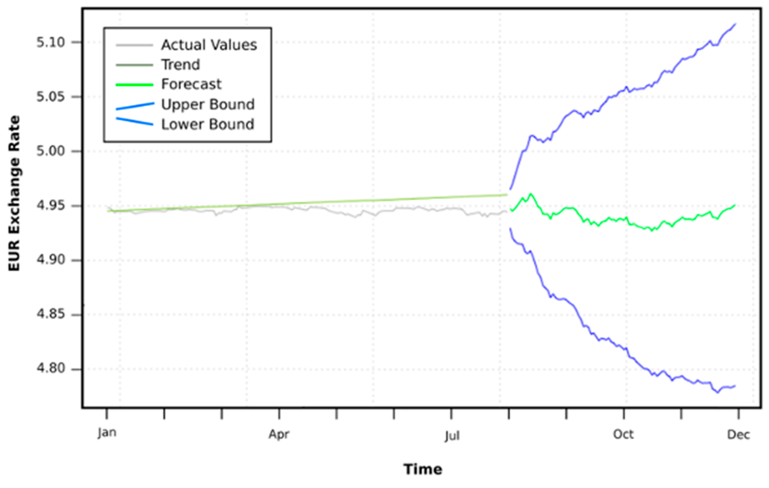
Figure 13 presents the results of the forecast for the last months (August–December) of 2022, which takes into account the time series of EUR exchange rate fluctuations for the first 7 months of 2022, respectively, the beginning of January to the end of July 2022. The average value of the forecast is 4.948.

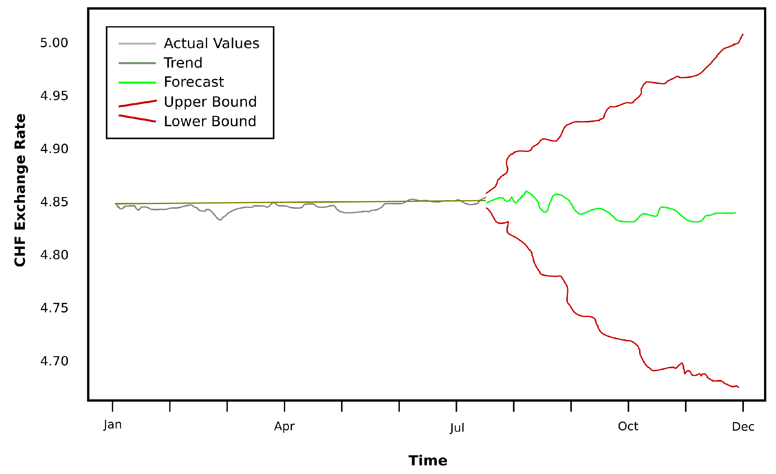
Figure 14 presents the results of the forecast for the last months (August–December) of 2022, which takes into account the time series of CHF exchange rate fluctuations for the first 7 months of 2022, respectively, the beginning of January to the end of July 2022. The average value of the forecast is 4.820.

Fractal trading hypotheses are used for price forecasting and improving stock market efficiency [18]. In addition, time series modeling and forecasting of the stock index in the NASDAQ stock exchange was discussed in the paper [19] using the ARMA–GARCH old consecrate model [20].

5. Conclusions

The nonlinear time series and fractal analysis method for financial data investigations has been successfully applied. The results frequently indicate that, in particular, the nonlinear structure is mostly verified. More exactly, both Swiss Franc (CHF) and Euro (EUR) currency evolutions (exchange rate) for a determined time period (during March–June 2022) were studied.

The fractal dimension evaluation has been performed by the technique of direct calculation as well as by the box-counting algorithm. The fractal dimensions are numerically calculated and graphically represented for CHF and EUR (‘Counted boxes vs. log scale of inverted box dimensions’ and ‘Fractal dimension vs. box counting dimensions’).

Qualitatively speaking, the fractal dimension for the CHF is slightly higher than for the EUR, in accordance with Figure 1 and Figure 3. Quantitatively, the determined numerical values are for Swiss Franc—D_CHF ≅ 1.66, respectively, for European currency—D_EUR ≅ 1.59, these being the maximum reference values.

The exchange rates for EUR-RON and CHF-RON during March–June 2022 were represented as time series and analyzed as such.

Regarding the extreme values, we can easily find the minimum value (min = 4.7080), followed by the maximum value (max = 4.9300) for CHF, respectively, find the minimum value (min = 4.9409), followed by the maximum value (max = 4.9490) for EUR.

The Hurst exponent for EUR is included between the values 0.477 and 0.539. The Hurst exponent for CHF is included between the values 0.481 and 0.527. We have distinct parts of the original series with different typologies and not a single typology for the entire series (Figure 5 and Figure 6). The positive autocorrelation corresponding to 1/2 < H < 1 indicates persistent behavior of the time series, while for H values between 0 < H < 1/2, the time series reveals antipersistent behavior (negative autocorrelation).

The fractal dimension calculated with the formula D₁ = 2 − HE for EUR is included between the values 1.461 and 1.523. Fractal dimension calculated with the formula D₂ = 2 − HE for CHF is included between the values 1.473 and 1.5519.

• Utilizing the machine learning algorithms on time series data, a more than reasonable prediction by the end of the year of the exchange rate for major currencies was prepared accurately.
• As seen from studying the time series, there is a marked tendency to impair the RON currency in comparison with the EUR currency. This observation shows us that analyzing and forecasting foreign exchange rates reduces the risk of dramatic fluctuations and decreases uncertainty in the market for foreign exchange. In this way, the most constant currency at foreign exchange can be established, so one can know the currency in which it can be invested during the period supported by the prediction.
• In the future, we will improve the time series statistics and develop the ability to extract data (fractal dimension and Hurst exponent) directly from the graphical representations. We will also improve the forecasting rate of the exchange rate based on the appropriate time series and the machine learning algorithms on studied time series data.

References

1. Mandelbrot, B. How long is the coast of Britain? Statistical self-similarity and fractional dimension. Science 1967, 156, 636–638. [Google Scholar] [CrossRef] [PubMed]
2. Falconer, K. Fractal Geometry: Mathematical Foundations and Applications; John Wiley & Sons: Hoboken, NJ, USA, 2004. [Google Scholar]
3. National Bank of Romania. Available online: https://www.google.com/search?client=firefox-b-d&q=RBN+Annual+Report2022Overview (accessed on 15 March 2023).
4. Mandelbrot, B.B. The Fractal Geometry of Nature; WH Freeman: New York, NY, USA, 1983. [Google Scholar]
5. Ciucu, S.C.; Paun, V.P. Financial Data Analysis Using Nonlinear Time Series Methods. Fluctuations Interpretation of Foreign Currency Exchange Rates. Univ. Politeh. Buchar. Sci. Bull. Ser. A Appl. Math. Phys. 2015, 77, 235–248. [Google Scholar]
6. Nichita, M.V.; Paun, M.A.; Paun, V.A.; Paun, V.P. Fractal Analysis of Brain Glial Cells. Fractal Dimension and Lacunarity. Univ. Politeh. Buchar. Sci. Bull. Ser. A Appl. Math. Phys. 2019, 81, 273–284. [Google Scholar]
7. Bouda, M.; Caplan, J.S.; Saiers, J.E. Box-counting dimension revisited: Presenting an efficient method of minimizing quantization error and an assessment of the self-similarity of structural root systems. Front. Plant Sci. 2016, 7, 149. [Google Scholar] [CrossRef] [PubMed]
8. Tsay, R.S. Analysis of Financial Time Series; John Wiley & Sons, Inc.: Hoboken, NJ, USA, 2002. [Google Scholar]
9. Blome, C.; Schoenherr, T. Supply chain risk management in financial crises—A multiple case-study approach, Int. J. Prod. Econ. 2011, 134, 43–57. [Google Scholar] [CrossRef]
10. Bordescu, D.; Paun, M.A.; Paun, V.A.; Paun, V.P. Fractal analysis of Neuroimagistic. Lacunarity degree, a precious indicator in the detection of Alzheimer’s disease. Univ. Politeh. Buchar. Sci. Bull. Ser. A Appl. Math. Phys. 2018, 80, 309–320. [Google Scholar]
11. Fuller, W. Introduction to Statistical Time Series; Wiley: New York, NY, USA, 1995. [Google Scholar]
12. Wigner, E.P. Symmetry and conservation laws. Proc. Natl. Acad. Sci. USA 1964, 51, 956. [Google Scholar] [CrossRef] [PubMed]
13. Hurst, H.E. Long-term storage of reservoirs: An experimental study. Trans. Am. Soc. Civ. Eng. 1951, 116, 770–799. [Google Scholar] [CrossRef]
14. Qian, B.; Rasheed, K. Hurst Exponent and financial market predictability. In Proceedings of the IASTED Conference on “Financial Engineering and Applications” (FEA 2004), Cambridge, MA, USA, 8–10 November 2004; pp. 203–209. [Google Scholar]
15. Paun, M.-A.; Paun, V.-A.; Paun, V.-P. Spatial Series and Fractal Analysis Associated with FractureBehaviour of UO2 Ceramic Material. Fractal Fract. 2022, 6, 595. [Google Scholar] [CrossRef]
16. Savona, R.; Soumare, M.; Andersen, J.V. Financial Symmetry and Moods in the Market. PLoS ONE 2015, 10, e0118224. [Google Scholar] [CrossRef] [PubMed]
17. Kaibe, B.C.; O’Hara, J.G. Symmetry Analysis of an Interest Rate Derivatives PDE Model in Financial Mathematics. Symmetry 2019, 11, 1056. [Google Scholar] [CrossRef]
18. Blackledge, J.; Lamphiere, M. A Review of the Fractal Market Hypothesis for Trading and Market Price Prediction. Mathematics 2022, 10, 117. [Google Scholar] [CrossRef]
19. Arashi, M.; Rounaghi, M. Analysis of market efficiency and fractal feature of NASDAQ stock exchange: Time series modeling and forecasting of stock index using ARMA-GARCH model. Future Bus. J. 2022, 8, 14. [Google Scholar]
20. Kim, S.I. ARMA–GARCH model with fractional generalized hyperbolic innovations. Financ. Innov. 2022, 8, 48. [Google Scholar]
Figure 1. The fractal dimension versus box-counting dimension for CHF.
Symmetry 15 01896 g001
Figure 2. The fractal dimension versus log scale for CHF.
Symmetry 15 01896 g002
Figure 3. The fractal dimension versus box-counting dimension for EUR.
Symmetry 15 01896 g003
Figure 4. The fractal dimension versus log scale for EUR.
Symmetry 15 01896 g004
Figure 5. Exchange rate for EUR-RON during March–June 2022.
Symmetry 15 01896 g005
Figure 6. Exchange rate for CHF-RON during March–June 2022.
Symmetry 15 01896 g006
Figure 7. Hurst exponent for EUR, distinct values for 22 days.
Symmetry 15 01896 g007
Figure 8. Hurst exponent for CHF, distinct values for 22 days.
Symmetry 15 01896 g008
Figure 9. Fractal dimension D1 for EUR, distinct values for 22 days.
Symmetry 15 01896 g009
Figure 10. Fractal dimension D2 for CHF, distinct values for 22 days.
Symmetry 15 01896 g010
Figure 11. Hurst exponent H representative curves, the first for EUR, the second for CHF, and the third for EUR, but calculated with the formula H = 2 − D.
Symmetry 15 01896 g011
Figure 12. Symmetry of one steady and one unsteady supporting level (a represents the upper margin, b represents the lower margin).
Symmetry 15 01896 g012
Figure 13. EUR-RON exchange rate prognosis for the end of 2022.
Symmetry 15 01896 g013
Figure 14. CHF-RON exchange rate prognosis for the end of 2022.
Symmetry 15 01896 g014
Disclaimer/Publisher’s Note: The statements, opinions and data contained in all publications are solely those of the individual author(s) and contributor(s) and not of MDPI and/or the editor(s). MDPI and/or the editor(s) disclaim responsibility for any injury to people or property resulting from any ideas, methods, instructions or products referred to in the content.