Dynamics of Competitive Two-Strain Stochastic SIR Epidemics on Heterogeneous Networks

Abstract

Mathematical modeling in epidemiology, biology, and life sciences requires the use of stochastic models. In this paper, we derive a competitive two-strain stochastic SIR epidemic model by considering the change in state of the epidemic process due to an event. Based on the density-dependent process theory, we construct a six-dimensional deterministic model that can be used to describe the diffusion limit of the stochastic epidemic on a heterogeneous network. Furthermore, we show the explicit expressions for the variances of infectious individuals with strain 1 and strain 2 when the level of infection is increasing exponentially. In particular, we find that the expressions of the variances are symmetric. Finally, simulations for epidemics spreading on networks are performed to confirm our analytical results. We find a close agreement between the simulations and theoretical predictions.

1. Introduction

Infectious diseases caused by pathogens such as viruses and bacteria can spread between humans or animals. In real life, the emergence of new diseases and the persistence of existing diseases endanger human health and bring huge economic burdens to society. A century earlier, Kermack and Mckendrick had developed an SIR epidemic model for the single pathogen [1]. Since then, a very large number of models for epidemiology, biology, and life sciences have been formulated, analyzed, and employed [2,3,4].

Pathogens of diseases can be represented by multiple variants, and called by the general name strains. The presence of multiple strains of a pathogen makes it more difficult for us to combat the disease. For example, Haemophilus influenzae is represented by six serotypes: a, b, c, d, e, and f, as well as some variants that are not typeable. Dengue virus has four serotypes. COVID-19 has five variant strains, namely the Alpha variant, Beta variant, Gamma variant, Delta variant, and Omicron variant [5,6]. There have been many researchers who have studied multistrain infectious diseases and focused on symmetry in infectious diseases [7,8,9]. In particular, the interrelationship between different strains, such as competition, mutation, superinfection, and cross infection, has attracted much attention. For example, Ackleh and Allen argued that there is a competitive exclusion and coexistence of strains in gonorrhea and other sexually infectious diseases [10].

In addition, most mathematical models that describe the spread of multistrain diseases assume that all members of a population are uniformly mixing and ignore individual heterogeneity. A more realistic way is to consider the transmission of diseases through contacts between people, with these contacts describing a network of interactions [11,12,13,14]. There have been many examples of using networks to study epidemic models with multiple strains [15,16,17]. Yao and Zhang developed a two-strain SIS model on heterogeneous networks with demographics for disease transmission [16]. Chung and Lui proved the local asymptotic stability of the interior steady state of a two-strain influenza model with sufficiently close cross-immunity [17].

Observed epidemics are noisy and unpredictable, which motivates the use of stochastic epidemic models [8,18,19,20]. Firstly, under the same initial conditions, standard models based on ODEs predict the same results. By contrast, stochastic models can predict the variability of the level of infection by capturing the chance nature of the event. Secondly, the interaction of stochasticity with the natural oscillatory behaviour of epidemics can lead to a range of phenomena that differ from deterministic models. El Hajji considered a mathematical dynamical system involving both deterministic and stochastic SIR epidemic models with nonlinear incidence rates in a continuous reactor [20]. For the deterministic model, a profound qualitative analysis was given. For the stochastic model, the long-time dynamics were concluded using the Feller’s test combined with the canonical probability method. Chen and Kang studied a stochastic multi-strain SIS epidemic model by introducing Lévy noise into the disease transmission rate of each strain [8]. They found that Lévy noise can cause the two strains to be almost guaranteed to become extinct, even though there is a dominant strain that persists in the deterministic model. Unfortunately, they can only get the properties of solutions to the stochastic differential equation, such as the stochastic stability of the disease-free equilibrium and the existence of the unique positive solution. We are still unable to obtain the transient dynamics of the disease and analyze the variability of the level of infection. In addition, a wide body of literature has demonstrated that stochastic models can generate very different dynamics compared with deterministic models; however, heterogeneous differences have rarely been elucidated. Here, we offer an analytical insight into the confounding roles of stochasticity and network structure in the dynamics of infection.

In this paper, we will study a competitive two-strain stochastic SIR epidemic on a configuration model network. Using probability-generating functions, we obtain a six-dimensional stochastic model. Based on the density-dependent process theory, we derive analytical expressions for the variances of the early development phase of an epidemic on a network given its degree of distribution. In particular, we find that the expressions of the variances are symmetric. Simulations of the evolution of epidemics in various networks are implemented to confirm the usefulness of our analysis.

2. The Competitive Two-Strain Stochastic SIR Model

We use the configuration model network with the degree distribution $p_k$. The probability generating function of degree distribution $p_k$ is defined as $g\left(x\right)={\sum }_k{p}_k{x}^k,x\in [0,1]$. The average degree is ${\mu }_D$, ${\mu }_D={\sum }_{k=1}^{M}k{p}_k=g^{\prime }\left(1\right)$, where M is the maximum degree. Individuals are classified according to their disease states $\mathrm{S}$, $\mathrm{I}$, $\mathrm{J}$ or $\mathrm{R}$, and their degree on the network. For $k=1,\dots ,M$ and $t\ge 0$, let $\left[S_k\right]\left(t\right)$ be the number of susceptible individuals of degree k at time t. Similarly, $\left[I_k\right]\left(t\right)$ and $\left[J_k\right]\left(t\right)$ are the numbers of individuals of degree k infected by strain 1 and strain 2 at time t, respectively. For $t\ge 0$, let $\left[SS\right]\left(t\right)$, $\left[SI\right]\left(t\right)$ and $\left[SJ\right]\left(t\right)$ be the numbers of $\mathrm{S}-\mathrm{S}$, $\mathrm{S}-\mathrm{I}$ and $\mathrm{S}-\mathrm{J}$ pairs at time t, respectively. Let

$$\mathit{W}\left(t\right)=\left(\left[S_1\right]\left(t\right),\dots ,\left[S_M\right]\left(t\right),\left[I_1\right]\left(t\right),\dots ,\left[I_M\right]\left(t\right),\left[J_1\right]\left(t\right),\dots ,\left[J_M\right]\left(t\right),\left[SS\right]\left(t\right),\left[SI\right]\left(t\right),\left[SJ\right]\left(t\right)\right).$$

The state space of $\mathit{W}\left(t\right)$ is

$$\begin{array}{cc}\hfill H=\{& \left(\left[S_1\right],\dots ,\left[S_M\right],\left[I_1\right],\dots ,\left[I_M\right],\left[J_1\right],\dots ,\left[J_M\right],\left[SS\right],\left[SI\right],\left[SJ\right]\right):\left[S_k\right],\left[I_k\right],\left[J_k\right]\ge 0,\hfill \\ & \left[S_k\right]+\left[I_k\right]+\left[J_k\right]\le N_k,k=1,\dots ,M,\left[SS\right],\left[SI\right],\left[SJ\right]\ge 0,\left[SS\right]+\left[SI\right]+\left[SJ\right]\le {\mu }_{D}N\},\hfill \end{array}$$

where N is the total population size and $N_k$ is the number of individuals of degree k. Let $\left[S\right]\left(t\right)={\sum }_{k=1}^M\left[S_k\right]\left(t\right)$, $\left[I\right]\left(t\right)={\sum }_{k=1}^M\left[I_k\right]\left(t\right)$ and $\left[J\right]\left(t\right)={\sum }_{k=1}^M\left[J_k\right]\left(t\right)$. Thus, $\left[S\right]\left(t\right)$, $\left[I\right]\left(t\right)$ and $\left[J\right]\left(t\right)$ are the total numbers of susceptibles infected with strain 1 and strain 2 at time t, respectively.

To derive the two-strain SIR model, we must consider the neighbourhood of each node. Firstly, we make the following assumptions.

(i)

The distribution of neighbourhoods with x susceptibles, y infected with strain 1 and z infected with strain 2 around a susceptible node of degree k follows a multinomial, that is

$$P_{x,y,z,k}^S={\mathrm{C}}_k^{x,y,z}{p}_{S-S}^x{p}_{S-I}^y{p}_{S-J}^z{(1-p_{S-S}-p_{S-I}-p_{S-J})}^{k-x-y-z}$$

with

$$p_{S-S}=\frac{\left[SS\right]}{{\sum }_{k}k\left[S_k\right]},p_{S-I}=\frac{\left[SI\right]}{{\sum }_{k}k\left[S_k\right]},p_{S-J}=\frac{\left[SJ\right]}{{\sum }_{k}k\left[S_k\right]}.$$

For infectious nodes, we only focus on the susceptible neighbors. Thus,

(ii)

the distribution of neighbourhoods with x susceptibles around an infectious node with strain 1 of degree k follows a binomial, that is

$$P_{x,k}^I={\mathrm{C}}_k^x{p}_{I-S}^x{(1-p_{I-S})}^{k-x}$$

with

$$p_{I-S}=\frac{\left[SI\right]}{{\sum }_{k}k\left[I_k\right]};$$

(iii)

the distribution of neighbourhoods with x susceptibles around an infectious node with strain 2 of degree k follows a binomial, that is

$$P_{x,k}^J={\mathrm{C}}_k^x{p}_{J-S}^x{(1-p_{J-S})}^{k-x}$$

with

$$p_{J-S}=\frac{\left[SJ\right]}{{\sum }_{k}k\left[J_k\right]}.$$

The process $\left\{\mathit{W}\right(t\left)\right\}$ is a continuous time Markov chain. Let

$$\mathit{h}=\left(\left[S_1\right],\dots ,\left[S_M\right],\left[I_1\right],\dots ,\left[I_M\right],\left[J_1\right],\dots ,\left[J_M\right],\left[SS\right],\left[SI\right],\left[SJ\right]\right)$$

denote a typical element of H. There are four basic events: the infection of a susceptible node by an infectious node with strain 1 or strain 2, and the recovery of an infectious node with strain 1 or strain 2. Susceptible individuals are infected by one of their infected neighbors with strain 1 at rate ${\tau }_1$ or with strain 2 at rate ${\tau }_2$. Those infected with strain 1 recover at rate ${\gamma }_1$, and those infecteds with strain 2 recover at rate ${\gamma }_2$. There are four types of jump for $\left\{\mathit{W}\right(t\left)\right\}$,; for the transmission event (a susceptible node of degree k has x susceptible neighbours, y infected neighbours with strain 1, z infected neighbours with strain 2), the jumps are given by

$$\begin{array}{cc}\hfill {\mathit{l}}_{k1}=& \left(-{\delta }_{1k},\dots ,-{\delta }_{Mk},{\delta }_{1k},\dots ,{\delta }_{Mk},0,\dots ,0,-2x,x-y,-z\right),\hfill \\ \hfill {\mathit{l}}_{k2}=& \left(-{\delta }_{1k},\dots ,-{\delta }_{Mk},0,\dots ,0,{\delta }_{1k},\dots ,{\delta }_{Mk},-2x,-y,x-z\right),\hfill \end{array}$$

where ${\delta }_{mk}$$(m=1,\dots ,M)$ is the Kronecker delta symbol. For the recovery event (an infectious node of degree k with strain 1 or strain 2 has x susceptible neighbours), the jumps are given by

$$\begin{array}{cc}\hfill {\mathit{l}}_{k3}=& \left(0,\dots ,0,-{\delta }_{1k},\dots ,-{\delta }_{Mk},0,\dots ,0,0,-x,0\right),\hfill \\ \hfill {\mathit{l}}_{k4}=& \left(0,\dots ,0,0,\dots ,0,-{\delta }_{1k},\dots ,-{\delta }_{Mk},0,0,-x\right).\hfill \end{array}$$

The corresponding state transition rates of $\left\{\mathit{W}\right(t\left)\right\}$ are given below: a susceptible node of degree k (the node has x susceptible neighbours, y infected neighbours with strain 1, z infected neighbours with strain 2) is infected by one of his infected neighbors with strain 1 at rate

$$q(\mathit{h},\mathit{h} + {\mathit{l}}_{k1})={\tau }_{1}y\left[S_k\right]P_{x,y,z,k}^S;$$

a susceptible node of degree k is infected by one of his infected neighbors with strain 2 at rate

$$q(\mathit{h},\mathit{h} + {\mathit{l}}_{k2})={\tau }_{2}z\left[S_k\right]P_{x,y,z,k}^S;$$

an infected node of degree k with strain 1 recovers at rate

$$q(\mathit{h},\mathit{h} + {\mathit{l}}_{k3})={\gamma }_1\left[I_k\right]P_{x,k}^I;$$

an infected node of degree k with strain 2 recovers at rate

$$q(\mathit{h},\mathit{h} + {\mathit{l}}_{k4})={\gamma }_2\left[J_k\right]P_{x,k}^J.$$

Let ${\widehat{s}}_k=\left[S_k\right]/N$, ${\widehat{i}}_k=\left[I_k\right]/N$, ${\widehat{j}}_k=\left[J_k\right]/N$$(k=1,\dots ,M)$, $\widehat{u}=\left[SS\right]/N$, ${\widehat{v}}_1=\left[SI\right]/N$ and ${\widehat{v}}_2=\left[SJ\right]/N$. Note that, for a given degree k, the intensities of the jumps of $\left\{\mathit{W}\right(t\left)\right\}$ have the following form

$$q(\mathit{h},\mathit{h} + {\mathit{l}}_{km})=N{\beta }_{{\mathit{l}}_{km}}\left(\frac{\mathit{h}}{N}\right),m=1,\dots ,4,\mathit{h}\in H$$

with

$$\begin{array}{c}\hfill \begin{array}{c}\hfill \begin{array}{cc}\hfill {\beta }_{{\mathit{l}}_{k1}}({\widehat{s}}_1,\dots ,{\widehat{s}}_M,{\widehat{i}}_1,\dots ,{\widehat{i}}_M,{\widehat{j}}_1,\dots ,{\widehat{j}}_M,\widehat{u},{\widehat{v}}_1,{\widehat{v}}_2)=& {\tau }_{1}y{\widehat{s}}_k{\tilde{P}}_{x,y,z,k}^S,\hfill \\ \hfill {\beta }_{{\mathit{l}}_{k2}}({\widehat{s}}_1,\dots ,{\widehat{s}}_M,{\widehat{i}}_1,\dots ,{\widehat{i}}_M,{\widehat{j}}_1,\dots ,{\widehat{j}}_M,\widehat{u},{\widehat{v}}_1,{\widehat{v}}_2)=& {\tau }_{2}z{\widehat{s}}_k{\tilde{P}}_{x,y,z,k}^S,\hfill \\ \hfill {\beta }_{{\mathit{l}}_{k3}}({\widehat{s}}_1,\dots ,{\widehat{s}}_M,{\widehat{i}}_1,\dots ,{\widehat{i}}_M,{\widehat{j}}_1,\dots ,{\widehat{j}}_M,\widehat{u},{\widehat{v}}_1,{\widehat{v}}_2)=& {\gamma }_1{\widehat{i}}_k{\tilde{P}}_{x,k}^I,\hfill \\ \hfill {\beta }_{{\mathit{l}}_{k4}}({\widehat{s}}_1,\dots ,{\widehat{s}}_M,{\widehat{i}}_1,\dots ,{\widehat{i}}_M,{\widehat{j}}_1,\dots ,{\widehat{j}}_M,\widehat{u},{\widehat{v}}_1,{\widehat{v}}_2)=& {\gamma }_2{\widehat{j}}_k{\tilde{P}}_{x,k}^J,\hfill \end{array}\end{array}\end{array}$$

where

$$\begin{array}{c}\hfill \begin{array}{c}\hfill \begin{array}{cc}\hfill {\tilde{P}}_{x,y,z,k}^S=& {\mathrm{C}}_k^{x,y,z}{\left(\frac{\widehat{u}}{{\sum }_{m}m{\widehat{s}}_m}\right)}^x{\left(\frac{{\widehat{v}}_1}{{\sum }_{m}m{\widehat{s}}_m}\right)}^y{\left(\frac{{\widehat{v}}_2}{{\sum }_{m}m{\widehat{s}}_m}\right)}^z{\left(1-\frac{\widehat{u}}{{\sum }_{m}m{\widehat{s}}_m}-\frac{{\widehat{v}}_1}{{\sum }_{m}m{\widehat{s}}_m}-\frac{{\widehat{v}}_2}{{\sum }_{m}m{\widehat{s}}_m}\right)}^{k-x-y-z},\hfill \\ \hfill {\tilde{P}}_{x,k}^I=& {\mathrm{C}}_k^x{\left(\frac{{\widehat{v}}_1}{{\sum }_{m}m{\widehat{i}}_m}\right)}^x{\left(1-\frac{{\widehat{v}}_1}{{\sum }_{m}m{\widehat{i}}_m}\right)}^{k-x},\hfill \\ \hfill {\tilde{P}}_{x,k}^J=& {\mathrm{C}}_k^x{\left(\frac{{\widehat{v}}_2}{{\sum }_{m}m{\widehat{j}}_m}\right)}^x{\left(1-\frac{{\widehat{v}}_2}{{\sum }_{m}m{\widehat{j}}_m}\right)}^{k-x}.\hfill \end{array}\end{array}\end{array}$$

The deterministic process is denoted by $\mathit{w}\left(t\right)=\left(s_1\left(t\right),\dots ,s_M\left(t\right),i_1\left(t\right),\dots ,i_M\left(t\right),j_1\left(t\right),\dots \right.$, $\left.j_M\left(t\right),u\left(t\right),v_1\left(t\right),v_2\left(t\right)\right)$, where $s_k\left(t\right)=\left[S_k\right]\left(t\right)/N$, $i_k\left(t\right)=\left[I_k\right]\left(t\right)/N$, $j_k\left(t\right)=\left[J_k\right]\left(t\right)/N$$(k=1,\dots ,M)$, $u\left(t\right)=\left[SS\right]\left(t\right)/N$, $v_1\left(t\right)=\left[SI\right]\left(t\right)/N$ and $v_2\left(t\right)=\left[SJ\right]\left(t\right)/N$. Given the initial conditions $N^{-1}\mathit{W}\left(0\right)=(s_1\left(0\right),\dots ,s_M\left(0\right),i_1\left(0\right),\dots ,i_M\left(0\right),j_1\left(0\right),\dots$, $j_M\left(0\right),u\left(0\right),v_1\left(0\right),v_2\left(0\right))$. Based on the work of Kurtz [21], $\mathit{w}\left(t\right)$ is the solution of

$$\begin{array}{cc}\hfill \frac{\mathrm{d}\mathit{w}\left(t\right)}{\mathrm{d}t}=& \sum _{k,x,y,z}{\beta }_{{\mathit{l}}_{k1}}\left(\mathit{w}\right){\mathit{l}}_{k1}+\sum _{k,x,y,z}{\beta }_{{\mathit{l}}_{k2}}\left(\mathit{w}\right){\mathit{l}}_{k2}+\sum _{k,x}{\beta }_{{\mathit{l}}_{k3}}\left(\mathit{w}\right){\mathit{l}}_{k3}+\sum _{k,x}{\beta }_{{\mathit{l}}_{k4}}\left(\mathit{w}\right){\mathit{l}}_{k4}\hfill \\ \hfill =& {\tau }_1\sum _{k,x,y,z}y{s}_k{\tilde{P}}_{x,y,z,k}^S{\mathit{l}}_{k1}+{\tau }_2\sum _{k,x,y,z}z{s}_k{\tilde{P}}_{x,y,z,k}^S{\mathit{l}}_{k2}+{\gamma }_1\sum _{k,x}{i}_k{\tilde{P}}_{x,k}^I{\mathit{l}}_{k3}+{\gamma }_2\sum _{k,x}{j}_k{\tilde{P}}_{x,k}^J{\mathit{l}}_{k4}.\hfill \end{array}$$

Thus, we get the following deterministic system

$$\left\{\begin{array}{cc}\hfill \frac{\mathrm{d}{s}_n}{\mathrm{d}t}=& -{\tau }_{1}n{s}_n\frac{v_1}{{\sum }_{m}m{s}_m}-{\tau }_{2}n{s}_n\frac{v_2}{{\sum }_{m}m{s}_m},n=1,\dots ,M,\hfill \\ \hfill \frac{\mathrm{d}{i}_n}{\mathrm{d}t}=& {\tau }_{1}n{s}_n\frac{v_1}{{\sum }_{m}m{s}_m}-{\gamma }_1{i}_n,n=1,\dots ,M,\hfill \\ \hfill \frac{\mathrm{d}{j}_n}{\mathrm{d}t}=& {\tau }_{2}n{s}_n\frac{v_2}{{\sum }_{m}m{s}_m}-{\gamma }_2{j}_n,n=1,\dots ,M,\hfill \\ \hfill \frac{\mathrm{d}u}{\mathrm{d}t}=& -2{\tau }_1\sum _{m}m(m-1)s_m\frac{u{v}_1}{{\left({\sum }_{m}m{s}_m\right)}^2}-2{\tau }_2\sum _{m}m(m-1)s_m\frac{u{v}_2}{{\left({\sum }_{m}m{s}_m\right)}^2},\hfill \\ \hfill \frac{\mathrm{d}{v}_1}{\mathrm{d}t}=& {\tau }_1\sum _{m}m(m-1)s_m\frac{u{v}_1}{{\left({\sum }_{m}m{s}_m\right)}^2}-{\tau }_1\sum _{m}m(m-1)s_m\frac{v_1^2}{{\left({\sum }_{m}m{s}_m\right)}^2}\hfill \\ \hfill & -{\tau }_2\sum _{m}m(m-1)s_m\frac{v_1{v}_2}{{\left({\sum }_{m}m{s}_m\right)}^2}-{\tau }_1{v}_1-{\gamma }_1{v}_1,\hfill \\ \hfill \frac{\mathrm{d}{v}_2}{\mathrm{d}t}=& {\tau }_2\sum _{m}m(m-1)s_m\frac{u{v}_2}{{\left({\sum }_{m}m{s}_m\right)}^2}-{\tau }_2\sum _{m}m(m-1)s_m\frac{v_2^2}{{\left({\sum }_{m}m{s}_m\right)}^2}\hfill \\ \hfill & -{\tau }_1\sum _{m}m(m-1)s_m\frac{v_1{v}_2}{{\left({\sum }_{m}m{s}_m\right)}^2}-{\tau }_2{v}_2-{\gamma }_2{v}_2.\hfill \end{array}\right.$$

(1)

Using the result of Kurtz [21], as $N\to \infty$, we know that for every $T\ge 0$,

$$\underset{N\to \infty }{lim}\underset{0\le t\le T}{sup}\mid N^{-1}\mathit{W}\left(t\right)-\mathit{w}\left(t\right)\mid =0\mathrm{almost}\mathrm{surely},$$

where $\mathit{w}\left(t\right)$ is the solution of a deterministic system (1) with initial condition $\mathit{w}\left(0\right)=$$N^{-1}\mathit{W}\left(0\right)$. Further,

$$\sqrt{N}\left(\left\{N^{-1}\mathit{W}\left(t\right)\right\}-\left\{\mathit{w}\left(t\right)\right\}\right)\Rightarrow \left\{\mathit{V}\left(t\right)\right\},$$

where ⇒ denotes weak convergence and $\left\{\mathit{V}\left(t\right)\right\}=\left\{\mathit{V}\left(t\right):t\ge 0\right\}$ is a zero-mean Gaussian process.

Let $s={\sum }_{n=1}^M{s}_n$, $i={\sum }_{n=1}^M{i}_n$ and $j={\sum }_{n=1}^M{j}_n$. Lumping together the differential equations for $s_n$, $i_n$ and $j_n$, we obtain

$$\left\{\begin{array}{cc}\hfill \frac{\mathrm{d}s}{\mathrm{d}t}=& -{\tau }_1{v}_1-{\tau }_2{v}_2,\hfill \\ \hfill \frac{\mathrm{d}i}{\mathrm{d}t}=& {\tau }_1{v}_1-{\gamma }_{1}i,\hfill \\ \hfill \frac{\mathrm{d}j}{\mathrm{d}t}=& {\tau }_2{v}_2-{\gamma }_{2}j,\hfill \\ \hfill \frac{\mathrm{d}u}{\mathrm{d}t}=& -2{\tau }_1\sum _{m}m(m-1)s_m\frac{u{v}_1}{{\left({\sum }_{m}m{s}_m\right)}^2}-2{\tau }_2\sum _{m}m(m-1)s_m\frac{u{v}_2}{{\left({\sum }_{m}m{s}_m\right)}^2},\hfill \\ \hfill \frac{\mathrm{d}{v}_1}{\mathrm{d}t}=& {\tau }_1\sum _{m}m(m-1)s_m\frac{u{v}_1}{{\left({\sum }_{m}m{s}_m\right)}^2}-{\tau }_1\sum _{m}m(m-1)s_m\frac{v_1^2}{{\left({\sum }_{m}m{s}_m\right)}^2}\hfill \\ \hfill & -{\tau }_2\sum _{m}m(m-1)s_m\frac{v_1{v}_2}{{\left({\sum }_{m}m{s}_m\right)}^2}-{\tau }_1{v}_1-{\gamma }_1{v}_1,\hfill \\ \hfill \frac{\mathrm{d}{v}_2}{\mathrm{d}t}=& {\tau }_2\sum _{m}m(m-1)s_m\frac{u{v}_2}{{\left({\sum }_{m}m{s}_m\right)}^2}-{\tau }_2\sum _{m}m(m-1)s_m\frac{v_2^2}{{\left({\sum }_{m}m{s}_m\right)}^2}\hfill \\ \hfill & -{\tau }_1\sum _{m}m(m-1)s_m\frac{v_1{v}_2}{{\left({\sum }_{m}m{s}_m\right)}^2}-{\tau }_2{v}_2-{\gamma }_2{v}_2.\hfill \end{array}\right.$$

(2)

Inspired by the literature [18,22], we will reduce a relatively low dimensional network-based epidemic model by using the probability generating function. Let $\theta =\left[S_1\right]/\left(N{p}_1\right)=s_1/p_1$ represent the probability that a node having degree 1 remains susceptible at time t. The infection down each link is assumed to be independent, thus we have $\left[S_k\right]=N{p}_k{\theta }^k$ and $\left[S\right]=N{\sum }_k{p}_k{\theta }^k=Ng\left(\theta \right)$. Further, we have $s_k=p_k{\theta }^k$, $s=g\left(\theta \right)$, ${\sum }_{k}k{s}_k=\theta g^{\prime }\left(\theta \right)$ and ${\sum }_{k}k(k-1)s_k={\theta }^2{g}^{\prime \prime }\left(\theta \right)$. Thus, system (2) becomes

$$\left\{\begin{array}{cc}\hfill \frac{\mathrm{d}\theta }{\mathrm{d}t}=& -{\tau }_1\frac{v_1}{g^{\prime }\left(\theta \right)}-{\tau }_2\frac{v_2}{g^{\prime }\left(\theta \right)},\hfill \\ \hfill \frac{\mathrm{d}i}{\mathrm{d}t}=& {\tau }_1{v}_1-{\gamma }_{1}i,\hfill \\ \hfill \frac{\mathrm{d}j}{\mathrm{d}t}=& {\tau }_2{v}_2-{\gamma }_{2}j,\hfill \\ \hfill \frac{\mathrm{d}u}{\mathrm{d}t}=& -2{\tau }_{1}u{v}_1\frac{g^{\prime \prime }\left(\theta \right)}{g^{\prime }{\left(\theta \right)}^2}-2{\tau }_{2}u{v}_2\frac{g^{\prime \prime }\left(\theta \right)}{g^{\prime }{\left(\theta \right)}^2},\hfill \\ \hfill \frac{\mathrm{d}{v}_1}{\mathrm{d}t}=& {\tau }_{1}u{v}_1\frac{g^{\prime \prime }\left(\theta \right)}{g^{\prime }{\left(\theta \right)}^2}-{\tau }_1{v}_1^2\frac{g^{\prime \prime }\left(\theta \right)}{g^{\prime }{\left(\theta \right)}^2}-{\tau }_2{v}_1{v}_2\frac{g^{\prime \prime }\left(\theta \right)}{g^{\prime }{\left(\theta \right)}^2}-{\tau }_1{v}_1-{\gamma }_1{v}_1,\hfill \\ \hfill \frac{\mathrm{d}{v}_2}{\mathrm{d}t}=& {\tau }_{2}u{v}_2\frac{g^{\prime \prime }\left(\theta \right)}{g^{\prime }{\left(\theta \right)}^2}-{\tau }_2{v}_2^2\frac{g^{\prime \prime }\left(\theta \right)}{g^{\prime }{\left(\theta \right)}^2}-{\tau }_1{v}_1{v}_2\frac{g^{\prime \prime }\left(\theta \right)}{g^{\prime }{\left(\theta \right)}^2}-{\tau }_2{v}_2-{\gamma }_2{v}_2.\hfill \end{array}\right.$$

(3)

Let $\tilde{\mathit{W}}\left(t\right)=\left(\left[S_1\right]\left(t\right)/p_1,\left[I\right]\left(t\right),\left[J\right]\left(t\right),\left[SS\right]\left(t\right),\left[SI\right]\left(t\right),\left[SJ\right]\left(t\right)\right)$ and $\tilde{\mathit{w}}\left(t\right)=(\theta \left(t\right),i\left(t\right)$, $j\left(t\right),u\left(t\right),v_1\left(t\right),v_2\left(t\right))$. Instead of $\left\{\mathit{W}\right(t\left)\right\}$, we simply need to consider process $\left\{\tilde{\mathit{W}}\left(t\right)\right\}$. For the transmission event (a susceptible node of degree k has x susceptible neighbours, y infected neighbours with strain 1, z infected neighbours with strain 2), the jumps are given by

$$\begin{array}{cc}\hfill {\tilde{\mathit{l}}}_{k1}=& \left(-{\delta }_{1k}/p_1,1,0,-2x,x-y,-z\right),\hfill \\ \hfill {\tilde{\mathit{l}}}_{k2}=& \left(-{\delta }_{1k}/p_1,0,1,-2x,-y,x-z\right),\hfill \end{array}$$

For the recovery event (an infectious node of degree k with strain 1 or strain 2 has x susceptible neighbours), the jumps are given by

$$\begin{array}{cc}\hfill {\tilde{\mathit{l}}}_{k3}=& \left(0,-1,0,0,-x,0\right),\hfill \\ \hfill {\tilde{\mathit{l}}}_{k4}=& \left(0,0,-1,0,0,-x\right).\hfill \end{array}$$

The intensities of the jumps of $\left\{\tilde{\mathit{W}}\left(t\right)\right\}$ are given by

$$\begin{array}{cc}\hfill {\tilde{\beta }}_{{\tilde{\mathit{l}}}_{k1}}({\widehat{s}}_1/p_1,\widehat{i},\widehat{j},\widehat{u},{\widehat{v}}_1,{\widehat{v}}_2)=& {\tau }_{1}y{\widehat{s}}_k{\tilde{P}}_{x,y,z,k}^S,\hfill \\ \hfill {\tilde{\beta }}_{{\tilde{\mathit{l}}}_{k2}}({\widehat{s}}_1/p_1,\widehat{i},\widehat{j},\widehat{u},{\widehat{v}}_1,{\widehat{v}}_2)=& {\tau }_{2}z{\widehat{s}}_k{\tilde{P}}_{x,y,z,k}^S,\hfill \\ \hfill {\tilde{\beta }}_{{\tilde{\mathit{l}}}_{k3}}({\widehat{s}}_1/p_1,\widehat{i},\widehat{j},\widehat{u},{\widehat{v}}_1,{\widehat{v}}_2)=& {\gamma }_1{\widehat{i}}_k{\tilde{P}}_{x,k}^I,\hfill \\ \hfill {\tilde{\beta }}_{{\tilde{\mathit{l}}}_{k4}}({\widehat{s}}_1/p_1,\widehat{i},\widehat{j},\widehat{u},{\widehat{v}}_1,{\widehat{v}}_2)=& {\gamma }_2{\widehat{j}}_k{\tilde{P}}_{x,k}^J.\hfill \end{array}$$

Given the initial condition $N^{-1}\tilde{\mathit{W}}\left(0\right)=\left(\theta \left(0\right),i\left(0\right),j\left(0\right),u\left(0\right),v_1\left(0\right),v_2\left(0\right)\right)$, where $\theta \left(0\right)=s_1\left(0\right)/p_1$, $i\left(0\right)={\sum }_m{i}_m\left(0\right)$ and $j\left(0\right)={\sum }_m{j}_m\left(0\right)$. Similarly, as $N\to \infty$, for every $T\ge 0$,

$$\underset{N\to \infty }{lim}\underset{0\le t\le T}{sup}\mid N^{-1}\tilde{\mathit{W}}\left(t\right)-\tilde{\mathit{w}}\left(t\right)\mid =0\mathrm{almost}\mathrm{surely},$$

where $\tilde{\mathit{w}}\left(t\right)$ is the solution of a deterministic system (3) with initial condition $\tilde{\mathit{w}}\left(0\right)=N^{-1}\tilde{\mathit{W}}\left(0\right)$. Further, we have

$$\sqrt{N}\left(\left\{N^{-1}\tilde{\mathit{W}}\left(t\right)\right\}-\left\{\tilde{\mathit{w}}\left(t\right)\right\}\right)\Rightarrow \left\{\tilde{\mathit{V}}\left(t\right)\right\},$$

where ⇒ denotes weak convergence and $\left\{\tilde{\mathit{V}}\left(t\right)\right\}=\left\{\tilde{\mathit{V}}\left(t\right):t\ge 0\right\}$ is a zero-mean Gaussian process with variance function given by

$$\Sigma \left(t\right)=\mathrm{Var}\left(\tilde{\mathit{V}}\left(t\right)\right)=M\left(t\right)\left[{\int }_0^t{M}^{-1}\left(u\right)G\left(u\right){\left(M^{-1}\left(u\right)\right)}^{\top }\mathrm{d}u\right]{\left(M\left(t\right)\right)}^{\top },$$

(4)

where

$$M\left(t\right)=exp\left({\int }_0^{t}B\left(u\right)\mathrm{d}u\right)$$

with

$$B\left(t\right)=\nabla F\left(t\right).$$

$F\left(t\right)$ is the vector field of system (3), and

$$G\left(t\right)=\sum _{k,x,y,z}{\tilde{\beta }}_{{\tilde{\mathit{l}}}_{k1}}\left(\tilde{\mathit{w}}\right){\tilde{\mathit{l}}}_{k1}^{\top }{\tilde{\mathit{l}}}_{k1}+\sum _{k,x,y,z}{\tilde{\beta }}_{{\tilde{\mathit{l}}}_{k2}}\left(\tilde{\mathit{w}}\right){\tilde{\mathit{l}}}_{k2}^{\top }{\tilde{\mathit{l}}}_{k2}+\sum _{k,x}{\tilde{\beta }}_{{\tilde{\mathit{l}}}_{k3}}\left(\tilde{\mathit{w}}\right){\tilde{\mathit{l}}}_{k3}^{\top }{\tilde{\mathit{l}}}_{k3}+\sum _{k,x}{\tilde{\beta }}_{{\tilde{\mathit{l}}}_{k4}}\left(\tilde{\mathit{w}}\right){\tilde{\mathit{l}}}_{k4}^{\top }{\tilde{\mathit{l}}}_{k4}.$$

(5)

It follows that $\Sigma \left(t\right)$ satisfies

$$\frac{\mathrm{d}\Sigma \left(t\right)}{\mathrm{d}t}=G\left(t\right)+B\left(t\right)\Sigma \left(t\right)+\Sigma \left(t\right)B{\left(t\right)}^{\top }$$

with initial condition $\Sigma \left(0\right)=0$. Thus, $\Sigma \left(t\right)$ can be computed numerically.

3. Early Growth Behaviour

We analyze the variances of the prevalence of infections with strain 1 and strain 2 during the early development of the epidemic. A linearizing system (3) allows us to get a new system

$$\left\{\begin{array}{cc}\hfill \frac{\mathrm{d}\theta }{\mathrm{d}t}=& -\frac{{\tau }_1}{g^{\prime }\left(1\right)}{v}_1-\frac{{\tau }_2}{g^{\prime }\left(1\right)}{v}_2,\hfill \\ \hfill \frac{\mathrm{d}i}{\mathrm{d}t}=& {\tau }_1{v}_1-{\gamma }_{1}i,\hfill \\ \hfill \frac{\mathrm{d}j}{\mathrm{d}t}=& {\tau }_2{v}_2-{\gamma }_{2}j,\hfill \\ \hfill \frac{\mathrm{d}u}{\mathrm{d}t}=& -2{\tau }_1\frac{g^{\prime \prime }\left(1\right)}{g^{\prime }\left(1\right)}{v}_1-2{\tau }_2\frac{g^{\prime \prime }\left(1\right)}{g^{\prime }\left(1\right)}{v}_2,\hfill \\ \hfill \frac{\mathrm{d}{v}_1}{\mathrm{d}t}=& \left[{\tau }_1\frac{g^{\prime \prime }\left(1\right)}{g^{\prime }\left(1\right)}-{\tau }_1-{\gamma }_1\right]v_1,\hfill \\ \hfill \frac{\mathrm{d}{v}_2}{\mathrm{d}t}=& \left[{\tau }_2\frac{g^{\prime \prime }\left(1\right)}{g^{\prime }\left(1\right)}-{\tau }_2-{\gamma }_2\right]v_2.\hfill \end{array}\right.$$

(6)

To examine the dynamics, we assume that

$$\begin{array}{cc}\hfill i\left(t\right)& =i\left(0\right)exp\left(r_{1}t\right)=:\tilde{i}exp\left(r_{1}t\right),\hfill \\ \hfill j\left(t\right)& =j\left(0\right)exp\left(r_{2}t\right)=:\tilde{j}exp\left(r_{2}t\right),\hfill \end{array}$$

(7)

where $r_1,r_2>0$. Based on system (6), it follows that

$$\begin{array}{cc}\hfill \frac{\mathrm{d}i}{\mathrm{d}t}=& {\tau }_1{v}_1-{\gamma }_{1}i=r_{1}i,\hfill \\ \hfill \frac{\mathrm{d}j}{\mathrm{d}t}=& {\tau }_2{v}_2-{\gamma }_{2}j=r_{2}j.\hfill \end{array}$$

Thus,

$$\begin{array}{c}\hfill v_1=\frac{r_1+{\gamma }_1}{{\tau }_1}i,v_2=\frac{r_2+{\gamma }_2}{{\tau }_2}j.\end{array}$$

Moreover, we know that

$$\begin{array}{cc}\hfill \frac{\mathrm{d}{v}_1}{\mathrm{d}t}=& \left[{\tau }_1\frac{g^{\prime \prime }\left(1\right)}{g^{\prime }\left(1\right)}-{\tau }_1-{\gamma }_1\right]v_1=r_1{v}_1,\hfill \\ \hfill \frac{\mathrm{d}{v}_2}{\mathrm{d}t}=& \left[{\tau }_2\frac{g^{\prime \prime }\left(1\right)}{g^{\prime }\left(1\right)}-{\tau }_2-{\gamma }_2\right]v_2=r_2{v}_2.\hfill \end{array}$$

Hence,

$$\begin{array}{cc}\hfill {\tau }_1=& \frac{g^{\prime }\left(1\right)}{g^{\prime \prime }\left(1\right)-g^{\prime }\left(1\right)}(r_1+{\gamma }_1),{\tau }_2=\frac{g^{\prime }\left(1\right)}{g^{\prime \prime }\left(1\right)-g^{\prime }\left(1\right)}(r_2+{\gamma }_2).\hfill \end{array}$$

So, we have

$$\begin{array}{cc}\hfill v_1=& \frac{g^{\prime \prime }\left(1\right)-g^{\prime }\left(1\right)}{g^{\prime }\left(1\right)}i,\hfill \\ \hfill v_2=& \frac{g^{\prime \prime }\left(1\right)-g^{\prime }\left(1\right)}{g^{\prime }\left(1\right)}j.\hfill \end{array}$$

Using system (6), we then work out the early behaviour of the other variables,

$$\begin{array}{cc}\hfill \theta \left(t\right)& =1-\frac{r_1+{\gamma }_1}{r_1{g}^{\prime }\left(1\right)}i\left(t\right)-\frac{r_2+{\gamma }_2}{r_2{g}^{\prime }\left(1\right)}j\left(t\right),\hfill \\ \hfill u\left(t\right)& =g^{\prime }\left(1\right)-\frac{2g^{\prime \prime }\left(1\right)(r_1+{\gamma }_1)}{r_1{g}^{\prime }\left(1\right)}i\left(t\right)-\frac{2g^{\prime \prime }\left(1\right)(r_2+{\gamma }_2)}{r_2{g}^{\prime }\left(1\right)}j\left(t\right),\hfill \\ \hfill v_1\left(t\right)& =\frac{g^{\prime \prime }\left(1\right)-g^{\prime }\left(1\right)}{g^{\prime }\left(1\right)}i\left(t\right),\hfill \\ \hfill v_2\left(t\right)& =\frac{g^{\prime \prime }\left(1\right)-g^{\prime }\left(1\right)}{g^{\prime }\left(1\right)}j\left(t\right).\hfill \end{array}$$

(8)

It follows from (5) that

$$\begin{array}{cc}\hfill G\left(\mathit{w}\right)=& {\tau }_1\sum _{k,x,y,z}y{s}_k{\overline{P}}_{x,y,z,k}^S{T}_1+{\tau }_2\sum _{k,x,y,z}z{s}_k{\overline{P}}_{x,y,z,k}^S{T}_2+{\gamma }_1\sum _{k,x}{i}_k{\overline{P}}_{x,k}^I{T}_3+{\gamma }_2\sum _{k,x}{j}_k{\overline{P}}_{x,k}^J{T}_4,\hfill \end{array}$$

where

$$\begin{array}{cc}\hfill {\overline{P}}_{x,y,z,k}^S=& {\mathrm{C}}_k^{x,y,z}{\left(\frac{u}{\theta g^{\prime }\left(\theta \right)}\right)}^x{\left(\frac{v_1}{\theta g^{\prime }\left(\theta \right)}\right)}^y{\left(\frac{v_2}{\theta g^{\prime }\left(\theta \right)}\right)}^z\hfill \\ \hfill & \times {\left(1-\frac{u}{\theta g^{\prime }\left(\theta \right)}-\frac{v_1}{\theta g^{\prime }\left(\theta \right)}-\frac{v_2}{\theta g^{\prime }\left(\theta \right)}\right)}^{k-x-y-z},\hfill \\ \hfill {\overline{P}}_{x,k}^I=& {\mathrm{C}}_k^x{\left(\frac{v_1}{{\sum }_{m}m{i}_m}\right)}^x{\left(1-\frac{v_1}{{\sum }_{m}m{i}_m}\right)}^{k-x},\hfill \\ \hfill {\overline{P}}_{x,k}^J=& {\mathrm{C}}_k^x{\left(\frac{v_2}{{\sum }_{m}m{j}_m}\right)}^x{\left(1-\frac{v_2}{{\sum }_{m}m{j}_m}\right)}^{k-x},\hfill \end{array}$$

and

$$\begin{array}{c}\hfill T_1=\left(\begin{array}{cccccc}\frac{{\delta }_{1k}}{p_1^2}& -\frac{{\delta }_{1k}}{p_1}& 0& \frac{2x{\delta }_{1k}}{p_1}& \frac{(y-x){\delta }_{1k}}{p_1}& \frac{z{\delta }_{1k}}{p_1}\\ -\frac{{\delta }_{1k}}{p_1}& 1& 0& -2x& x-y& -z\\ 0& 0& 0& 0& 0& 0\\ \frac{2x{\delta }_{1k}}{p_1}& -2x& 0& 4x^2& 2x(y-x)& 2xz\\ \frac{(y-x){\delta }_{1k}}{p_1}& x-y& 0& 2x(y-x)& {(x-y)}^2& z(y-x)\\ \frac{z{\delta }_{1k}}{p_1}& -z& 0& 2xz& z(y-x)& z^2\end{array}\right),\end{array}$$

$$\begin{array}{c}\hfill T_2=\left(\begin{array}{cccccc}\frac{{\delta }_{1k}}{p_1^2}& 0& -\frac{{\delta }_{1k}}{p_1}& \frac{2x{\delta }_{1k}}{p_1}& \frac{y{\delta }_{1k}}{p_1}& \frac{(z-x){\delta }_{1k}}{p_1}\\ 0& 0& 0& 0& 0& 0\\ -\frac{{\delta }_{1k}}{p_1}& 0& 1& -2x& -y& x-z\\ \frac{2x{\delta }_{1k}}{p_1}& 0& -2x& 4x^2& 2xy& 2x(z-x)\\ \frac{y{\delta }_{1k}}{p_1}& 0& -y& 2xy& y^2& y(z-x)\\ \frac{(z-x){\delta }_{1k}}{p_1}& 0& x-z& 2x(z-x)& y(z-x)& {(x-z)}^2\end{array}\right),\end{array}$$

$$T_3=\left(\begin{array}{cccccc}0& 0& 0& 0& 0& 0\\ 0& 1& 0& 0& x& 0\\ 0& 0& 0& 0& 0& 0\\ 0& 0& 0& 0& 0& 0\\ 0& x& 0& 0& x^2& 0\\ 0& 0& 0& 0& 0& 0\end{array}\right),T_4=\left(\begin{array}{cccccc}0& 0& 0& 0& 0& 0\\ 0& 0& 0& 0& 0& 0\\ 0& 0& 1& 0& 0& x\\ 0& 0& 0& 0& 0& 0\\ 0& 0& 0& 0& 0& 0\\ 0& 0& x& 0& 0& x^2\end{array}\right).$$

Thus, we can obtain

$$\begin{array}{cc}\hfill G_{11}=& \frac{{\tau }_1}{p_1}\frac{v_1}{g^{\prime }\left(\theta \right)}+\frac{{\tau }_2}{p_1}\frac{v_2}{g^{\prime }\left(\theta \right)},G_{12}=G_{21}=-{\tau }_1\frac{v_1}{g^{\prime }\left(\theta \right)},G_{13}=G_{31}=-{\tau }_2\frac{v_2}{g^{\prime }\left(\theta \right)},\hfill \\ \hfill G_{14}=& G_{41}=0,G_{15}=G_{51}={\tau }_1\frac{v_1}{g^{\prime }\left(\theta \right)},G_{16}=G_{61}={\tau }_2\frac{v_2}{g^{\prime }\left(\theta \right)},\hfill \\ \hfill G_{22}=& {\tau }_1{v}_1+{\gamma }_{1}i,G_{23}=G_{32}=0,G_{24}=G_{42}=-2{\tau }_1\frac{g^{\prime \prime }\left(\theta \right)}{g^{\prime }{\left(\theta \right)}^2}u{v}_1,\hfill \\ \hfill G_{25}=& G_{52}={\tau }_1\frac{g^{\prime \prime }\left(\theta \right)}{g^{\prime }{\left(\theta \right)}^2}u{v}_1-{\tau }_1{v}_1-{\tau }_1\frac{g^{\prime \prime }\left(\theta \right)}{g^{\prime }{\left(\theta \right)}^2}{v}_1^2+{\gamma }_1{v}_1,\hfill \\ \hfill G_{26}=& G_{62}=-{\tau }_1\frac{g^{\prime \prime }\left(\theta \right)}{g^{\prime }{\left(\theta \right)}^2}{v}_1{v}_2,G_{33}={\tau }_2{v}_2+{\gamma }_{2}j,\hfill \\ \hfill G_{34}=& G_{43}=-2{\tau }_2\frac{g^{\prime \prime }\left(\theta \right)}{g^{\prime }{\left(\theta \right)}^2}u{v}_2,G_{35}=G_{53}=-{\tau }_2\frac{g^{\prime \prime }\left(\theta \right)}{g^{\prime }{\left(\theta \right)}^2}{v}_1{v}_2,\hfill \\ \hfill G_{36}=& G_{63}={\tau }_2\frac{g^{\prime \prime }\left(\theta \right)}{g^{\prime }{\left(\theta \right)}^2}u{v}_2-{\tau }_2{v}_2-{\tau }_2\frac{g^{\prime \prime }\left(\theta \right)}{g^{\prime }{\left(\theta \right)}^2}{v}_2^2+{\gamma }_2{v}_2,\hfill \end{array}$$

$$\begin{array}{cc}\hfill G_{44}=& 4{\tau }_1\frac{g^{\prime \prime \prime }\left(\theta \right)}{g^{\prime }{\left(\theta \right)}^3}{u}^2{v}_1+4{\tau }_1\frac{g^{\prime \prime }\left(\theta \right)}{g^{\prime }{\left(\theta \right)}^2}u{v}_1+4{\tau }_2\frac{g^{\prime \prime \prime }\left(\theta \right)}{g^{\prime }{\left(\theta \right)}^3}{u}^2{v}_2+4{\tau }_2\frac{g^{\prime \prime }\left(\theta \right)}{g^{\prime }{\left(\theta \right)}^2}u{v}_2,\hfill \\ \hfill G_{45}=& G_{54}=2{\tau }_1\frac{g^{\prime \prime \prime }\left(\theta \right)}{g^{\prime }{\left(\theta \right)}^3}u{v}_1^2-2{\tau }_1\frac{g^{\prime \prime \prime }\left(\theta \right)}{g^{\prime }{\left(\theta \right)}^3}{u}^2{v}_1+2{\tau }_2\frac{g^{\prime \prime \prime }\left(\theta \right)}{g^{\prime }{\left(\theta \right)}^3}u{v}_1{v}_2,\hfill \\ \hfill G_{46}=& G_{64}=2{\tau }_1\frac{g^{\prime \prime \prime }\left(\theta \right)}{g^{\prime }{\left(\theta \right)}^3}u{v}_1{v}_2+2{\tau }_2\frac{g^{\prime \prime \prime }\left(\theta \right)}{g^{\prime }{\left(\theta \right)}^3}u{v}_2^2-2{\tau }_2\frac{g^{\prime \prime \prime }\left(\theta \right)}{g^{\prime }{\left(\theta \right)}^3}{u}^2{v}_2,\hfill \\ \hfill G_{55}=& {\tau }_1\frac{g^{\prime \prime \prime }\left(\theta \right)}{g^{\prime }{\left(\theta \right)}^3}{u}^2{v}_1-2{\tau }_1\frac{g^{\prime \prime \prime }\left(\theta \right)}{g^{\prime }{\left(\theta \right)}^3}u{v}_1^2-{\tau }_1\frac{g^{\prime \prime }\left(\theta \right)}{g^{\prime }{\left(\theta \right)}^2}u{v}_1+{\tau }_1\frac{g^{\prime \prime \prime }\left(\theta \right)}{g^{\prime }{\left(\theta \right)}^3}{v}_1^3\hfill \\ \hfill & +3{\tau }_1\frac{g^{\prime \prime }\left(\theta \right)}{g^{\prime }{\left(\theta \right)}^2}{v}_1^2+{\tau }_1{v}_1+{\tau }_2\frac{g^{\prime \prime \prime }\left(\theta \right)}{g^{\prime }{\left(\theta \right)}^3}{v}_1^2{v}_2+{\tau }_2\frac{g^{\prime \prime }\left(\theta \right)}{g^{\prime }{\left(\theta \right)}^2}{v}_1{v}_2+{\gamma }_1\sum _{k,x}{x}^2{i}_k{\overline{P}}_{x,k}^I,\hfill \\ \hfill G_{56}=& G_{65}={\tau }_1\frac{g^{\prime \prime \prime }\left(\theta \right)}{g^{\prime }{\left(\theta \right)}^3}{v}_1^2{v}_2+{\tau }_1\frac{g^{\prime \prime }\left(\theta \right)}{g^{\prime }{\left(\theta \right)}^2}{v}_1{v}_2-{\tau }_1\frac{g^{\prime \prime \prime }\left(\theta \right)}{g^{\prime }{\left(\theta \right)}^3}u{v}_1{v}_2+{\tau }_2\frac{g^{\prime \prime \prime }\left(\theta \right)}{g^{\prime }{\left(\theta \right)}^3}{v}_1{v}_2^2\hfill \\ \hfill & +{\tau }_2\frac{g^{\prime \prime }\left(\theta \right)}{g^{\prime }{\left(\theta \right)}^2}{v}_1{v}_2-{\tau }_2\frac{g^{\prime \prime \prime }\left(\theta \right)}{g^{\prime }{\left(\theta \right)}^3}u{v}_1{v}_2,\hfill \\ \hfill G_{66}=& {\tau }_1\frac{g^{\prime \prime \prime }\left(\theta \right)}{g^{\prime }{\left(\theta \right)}^3}{v}_1{v}_2^2+{\tau }_1\frac{g^{\prime \prime }\left(\theta \right)}{g^{\prime }{\left(\theta \right)}^2}{v}_1{v}_2+{\tau }_2\frac{g^{\prime \prime \prime }\left(\theta \right)}{g^{\prime }{\left(\theta \right)}^3}{u}^2{v}_2-2{\tau }_2\frac{g^{\prime \prime \prime }\left(\theta \right)}{g^{\prime }{\left(\theta \right)}^3}u{v}_2^2-{\tau }_2\frac{g^{\prime \prime }\left(\theta \right)}{g^{\prime }{\left(\theta \right)}^2}u{v}_2\hfill \\ \hfill & +{\tau }_2\frac{g^{\prime \prime \prime }\left(\theta \right)}{g^{\prime }{\left(\theta \right)}^3}{v}_2^3+3{\tau }_2\frac{g^{\prime \prime }\left(\theta \right)}{g^{\prime }{\left(\theta \right)}^2}{v}_2^2+{\tau }_2{v}_2+{\gamma }_2\sum _{k,x}{x}^2{j}_k{\overline{P}}_{x,k}^J.\hfill \end{array}$$

Using (7) and (8), we linearise G with respect to $(i,j)$ at $(0,0)$. Then, we can obtain matrix G, where

$$\begin{array}{cc}\hfill G_{11}& =\frac{{\tau }_1}{p_1}\frac{g^{\prime \prime }-g^{\prime }}{g^{\prime 2}}i+\frac{{\tau }_2}{p_1}\frac{g^{\prime \prime }-g^{\prime }}{g^{\prime 2}}j,G_{12}=G_{21}=-{\tau }_1\frac{g^{\prime \prime }-g^{\prime }}{g^{\prime 2}}i,\hfill \\ \hfill G_{13}& =G_{31}=-{\tau }_2\frac{g^{\prime \prime }-g^{\prime }}{g^{\prime 2}}j,G_{14}=G_{41}=0,G_{15}=G_{51}={\tau }_1\frac{g^{\prime \prime }-g^{\prime }}{g^{\prime 2}}i,\hfill \\ \hfill G_{16}& =G_{61}={\tau }_2\frac{g^{\prime \prime }-g^{\prime }}{g^{\prime 2}}j,G_{22}=\left({\tau }_1\frac{g^{\prime \prime }}{g^{\prime }}-{\tau }_1+{\gamma }_1\right)i,G_{23}=G_{32}=0,\hfill \\ \hfill G_{24}& =G_{42}=-2{\tau }_1\frac{g^{\prime \prime }(g^{\prime \prime }-g^{\prime })}{g^{\prime 2}}i,G_{25}=G_{52}=\frac{(g^{\prime \prime }-g^{\prime })[{\tau }_1{g}^{\prime \prime }+({\gamma }_1-{\tau }_1)g^{\prime }]}{g^{\prime 2}}i,\hfill \\ \hfill G_{26}& =G_{62}=0,G_{33}=\left({\tau }_2\frac{g^{\prime \prime }}{g^{\prime }}-{\tau }_2+{\gamma }_2\right)j,\hfill \\ \hfill G_{34}& =G_{43}=-2{\tau }_2\frac{g^{\prime \prime }(g^{\prime \prime }-g^{\prime })}{g^{\prime 2}}j,G_{35}=G_{53}=0,\hfill \\ \hfill G_{36}& =G_{63}=\frac{(g^{\prime \prime }-g^{\prime })[{\tau }_2{g}^{\prime \prime }+({\gamma }_2-{\tau }_2)g^{\prime }]}{g^{\prime 2}}j,\hfill \\ \hfill G_{44}& =4{\tau }_1\frac{(g^{\prime \prime }-g^{\prime })(g^{\prime \prime \prime }+g^{\prime \prime })}{g^{\prime 2}}i+4{\tau }_2\frac{(g^{\prime \prime }-g^{\prime })(g^{\prime \prime \prime }+g^{\prime \prime })}{g^{\prime 2}}j,\hfill \\ \hfill G_{45}& =G_{54}=-2{\tau }_1\frac{g^{\prime \prime \prime }(g^{\prime \prime }-g^{\prime })}{g^{\prime 2}}i,G_{46}=G_{64}=-2{\tau }_2\frac{g^{\prime \prime \prime }(g^{\prime \prime }-g^{\prime })}{g^{\prime 2}}j,\hfill \end{array}$$

$$\begin{array}{cc}\hfill G_{55}& ={\tau }_1\frac{(g^{\prime \prime \prime }-g^{\prime \prime }+g^{\prime })(g^{\prime \prime }-g^{\prime })}{g^{\prime 2}}i+{\gamma }_1\sum _{k,x}{x}^2{i}_k{\overline{P}}_{x,k}^I,\hfill \\ \hfill G_{56}& =G_{65}=0,\hfill \\ \hfill G_{66}& ={\tau }_2\frac{(g^{\prime \prime \prime }-g^{\prime \prime }+g^{\prime })(g^{\prime \prime }-g^{\prime })}{g^{\prime 2}}j+{\gamma }_2\sum _{k,x}{x}^2{j}_k{\overline{P}}_{x,k}^J.\hfill \end{array}$$

Here, we have used the fact that $g^{\prime }\left(\theta \right)$, $g^{\prime \prime }\left(\theta \right)$ and $g^{\prime \prime \prime }\left(\theta \right)$ will become $g^{\prime }\left(1\right)$, $g^{\prime \prime }\left(1\right)$ and $g^{\prime \prime \prime }\left(1\right)$ with the use of the early growth assumption. Write $g^{\left(n\right)}\equiv g^{\left(n\right)}\left(1\right),n=1,2,3$. Next, we calculate ${\sum }_{k,x}{x}^2{i}_k{\overline{P}}_{x,k}^I$ and ${\sum }_{k,x}{x}^2{j}_k{\overline{P}}_{x,k}^J$.

Note that

$$\begin{array}{cc}\hfill \frac{\mathrm{d}{s}_k}{\mathrm{d}t}=& k{p}_k{\theta }^{k-1}\dot{\theta },\hfill \\ \hfill \frac{\mathrm{d}\theta }{\mathrm{d}t}=& -\frac{{\tau }_1}{g^{\prime }}{v}_1-\frac{{\tau }_2}{g^{\prime }}{v}_2=-\frac{r_1+{\gamma }_1}{g^{\prime }}i-\frac{r_2+{\gamma }_2}{g^{\prime }}j.\hfill \end{array}$$

Thus,

$$\begin{array}{c}\hfill \frac{\mathrm{d}{s}_k}{\mathrm{d}t}=-k{p}_k{\theta }^{k-1}\frac{r_1+{\gamma }_1}{g^{\prime }}i-k{p}_k{\theta }^{k-1}\frac{r_2+{\gamma }_2}{g^{\prime }}j.\end{array}$$

(9)

It follows from (9) that

$$\begin{array}{cc}\hfill i_k\left(t\right)=& i_k\left(0\right)+k{p}_k\frac{r_1+{\gamma }_1}{g^{\prime }}{\int }_0^t{\left(\theta (t-a)\right)}^{k-1}i(t-a){\mathrm{e}}^{-{\gamma }_{1}a}\mathrm{d}a\hfill \\ \hfill \approx & k{p}_k\frac{r_1+{\gamma }_1}{g^{\prime }}{\int }_0^t{\left(\theta (t-a)\right)}^{k-1}i(t-a){\mathrm{e}}^{-{\gamma }_{1}a}\mathrm{d}a,\hfill \\ \hfill j_k\left(t\right)=& j_k\left(0\right)+k{p}_k\frac{r_2+{\gamma }_2}{g^{\prime }}{\int }_0^t{\left(\theta (t-a)\right)}^{k-1}j(t-a){\mathrm{e}}^{-{\gamma }_{2}a}\mathrm{d}a\hfill \\ \hfill \approx & k{p}_k\frac{r_2+{\gamma }_2}{g^{\prime }}{\int }_0^t{\left(\theta (t-a)\right)}^{k-1}j(t-a){\mathrm{e}}^{-{\gamma }_{2}a}\mathrm{d}a,\hfill \end{array}$$

where ${\mathrm{e}}^{-{\gamma }_{1}a}$ is the probability that an infective of age a with strain 1 is still infective, and ${\mathrm{e}}^{-{\gamma }_{2}a}$ is the probability that an infective of age a with strain 2 is still infective.

Now consider the neighbourhood around such an infective with strain 1. Every infectious individual of degree k must have been infected by one of their infected neighbors, leaving $k-1$ individuals who are potentially susceptible. If the infection of the central node happened a time a ago, then each of the $k-1$ potentially susceptible neighbours has an independent probability ${\mathrm{e}}^{-{\tau }_{1}a}$ of avoiding infection from the central node. In addition, the neighbouring node of degree l has a probability of ${\theta }^{l-1}$ of avoiding infection from any other source. Summing over l, then, gives the general expression

$$\begin{array}{cc}\hfill i_k{\overline{P}}_{x,k}^I=& k{p}_k\frac{r_1+{\gamma }_1}{g^{\prime }}{\int }_0^t{\left(\theta (t-a)\right)}^{k-1}i(t-a){\mathrm{e}}^{-{\gamma }_{1}a}\hfill \\ \hfill & \times {\mathrm{C}}_k^x{\left(\frac{g^{\prime }\left(\theta \right)}{g^{\prime }\left(1\right)}{\mathrm{e}}^{-{\tau }_{1}a}\right)}^x{\left(1-\frac{g^{\prime }\left(\theta \right)}{g^{\prime }\left(1\right)}{\mathrm{e}}^{-{\tau }_{1}a}\right)}^{k-1-x}\mathrm{d}a.\hfill \end{array}$$

In the early growth phase of the infection, we assume that $\theta \approx 1$ and $g^{\prime }\left(\theta \right)\approx g^{\prime }\left(1\right)$. Hence,

$$\begin{array}{cc}\hfill \sum _{k,x}{x}^2{i}_k{\overline{P}}_{x,k}^I=& \sum _{k,x}{x}^{2}k{p}_k\frac{r_1+{\gamma }_1}{g^{\prime }}{\int }_0^{t}i(t-a){\mathrm{e}}^{-{\gamma }_{1}a}\hfill \\ \hfill & \times \left(\genfrac{}{}{0pt}{}{k-1}{x}\right){\left({\mathrm{e}}^{-{\tau }_{1}a}\right)}^x{\left(1-{\mathrm{e}}^{-{\tau }_{1}a}\right)}^{k-1-x}\mathrm{d}a\hfill \\ \hfill =& \frac{r_1+{\gamma }_1}{g^{\prime }}\sum _{k}k{p}_k{\int }_0^{t}i(t-a){\mathrm{e}}^{-{\gamma }_{1}a}\hfill \\ \hfill & \times \sum _x{x}^2\left(\genfrac{}{}{0pt}{}{k-1}{x}\right){\left({\mathrm{e}}^{-{\tau }_{1}a}\right)}^x{\left(1-{\mathrm{e}}^{-{\tau }_{1}a}\right)}^{k-1-x}\mathrm{d}a\hfill \\ \hfill =& \frac{r_1+{\gamma }_1}{g^{\prime }}i\sum _{k}k(k-1)(k-2)p_k{\int }_0^t{\mathrm{e}}^{-(2{\tau }_1+r_1+{\gamma }_1)a}\mathrm{d}a\hfill \\ \hfill & +\frac{r_1+{\gamma }_1}{g^{\prime }}i\sum _{k}k(k-1)p_k{\int }_0^t{\mathrm{e}}^{-({\tau }_1+r_1+{\gamma }_1)a}\mathrm{d}a\hfill \\ \hfill \approx & \frac{r_1+{\gamma }_1}{g^{\prime }}\left(\frac{g^{\prime \prime \prime }}{2{\tau }_1+r_1+{\gamma }_1}+\frac{g^{\prime \prime }}{{\tau }_1+r_1+{\gamma }_1}\right)i.\hfill \end{array}$$

Similarly, for an infective with strain 2, we can obtain

$$\begin{array}{cc}\hfill \sum _{k,x}{x}^2{j}_k{\overline{P}}_{x,k}=& \sum _{k,x}{x}^{2}k{p}_k\frac{r_2+{\gamma }_2}{g^{\prime }}{\int }_0^{t}j(t-a){\mathrm{e}}^{-{\gamma }_{2}a}\hfill \\ \hfill & \times \left(\genfrac{}{}{0pt}{}{k-1}{x}\right){\left({\mathrm{e}}^{-{\tau }_{2}a}\right)}^x{\left(1-{\mathrm{e}}^{-{\tau }_{2}a}\right)}^{k-1-x}\mathrm{d}a\hfill \\ \hfill \approx & \frac{r_2+{\gamma }_2}{g^{\prime }}\left(\frac{g^{\prime \prime \prime }}{2{\tau }_2+r_2+{\gamma }_2}+\frac{g^{\prime \prime }}{{\tau }_2+r_2+{\gamma }_2}\right)j.\hfill \end{array}$$

Therefore,

$$\begin{array}{cc}\hfill G_{55}=& {\tau }_1\frac{g^{\prime \prime }-g^{\prime }}{g^{\prime 2}}\left[g^{\prime \prime \prime }-g^{\prime \prime }+g^{\prime }+{\gamma }_1\left(\frac{g^{\prime \prime \prime }}{2{\tau }_1+r_1+{\gamma }_1}+\frac{g^{\prime \prime }}{{\tau }_1+r_1+{\gamma }_1}\right)\right]i,\hfill \\ \hfill G_{66}=& {\tau }_2\frac{g^{\prime \prime }-g^{\prime }}{g^{\prime 2}}\left[g^{\prime \prime \prime }-g^{\prime \prime }+g^{\prime }+{\gamma }_2\left(\frac{g^{\prime \prime \prime }}{2{\tau }_2+r_2+{\gamma }_2}+\frac{g^{\prime \prime }}{{\tau }_2+r_2+{\gamma }_2}\right)\right]j.\hfill \end{array}$$

It is not hard to find that matrix G can be written as ${\tilde{G}}_{1}i\left(t\right)+{\tilde{G}}_{2}j\left(t\right)$, where

$${\tilde{G}}_1=\left(\begin{array}{cccccc}\frac{{\tau }_1}{p_1}\frac{g^{\prime \prime }-g^{\prime }}{g^{\prime 2}}& -{\tau }_1\frac{g^{\prime \prime }-g^{\prime }}{g^{\prime 2}}& 0& 0& {\tau }_1\frac{g^{\prime \prime }-g^{\prime }}{g^{\prime 2}}& 0\\ -{\tau }_1\frac{g^{\prime \prime }-g^{\prime }}{g^{\prime 2}}& {\tau }_1\frac{g^{\prime \prime }}{g^{\prime }}-{\tau }_1+{\gamma }_1& 0& -2{\tau }_1\frac{g^{\prime \prime }(g^{\prime \prime }-g^{\prime })}{g^{\prime 2}}& \frac{(g^{\prime \prime }-g^{\prime })[{\tau }_1{g}^{\prime \prime }+({\gamma }_1-{\tau }_1)g^{\prime }]}{g^{\prime 2}}& 0\\ 0& 0& 0& 0& 0& 0\\ 0& -2{\tau }_1\frac{g^{\prime \prime }(g^{\prime \prime }-g^{\prime })}{g^{\prime 2}}& 0& 4{\tau }_1\frac{(g^{\prime \prime }-g^{\prime })(g^{\prime \prime \prime }+g^{\prime \prime })}{g^{\prime 2}}& -2{\tau }_1\frac{g^{\prime \prime \prime }(g^{\prime \prime }-g^{\prime })}{g^{\prime 2}}& 0\\ {\tau }_1\frac{g^{\prime \prime }-g^{\prime }}{g^{\prime 2}}& \frac{(g^{\prime \prime }-g^{\prime })[{\tau }_1{g}^{\prime \prime }+({\gamma }_1-{\tau }_1)g^{\prime }]}{g^{\prime 2}}& 0& -2{\tau }_1\frac{g^{\prime \prime \prime }(g^{\prime \prime }-g^{\prime })}{g^{\prime 2}}& {\tau }_1\frac{(g^{\prime \prime }-g^{\prime })(g^{\prime \prime \prime }-g^{\prime \prime }+g^{\prime })+{\gamma }_1(g^{\prime \prime }-g^{\prime })\left(\frac{g^{\prime \prime }}{{\tau }_1+r_1+{\gamma }_1}+\frac{g^{\prime \prime \prime }}{2{\tau }_1+r_1+{\gamma }_1}\right)}{g^{\prime 2}}& 0\\ 0& 0& 0& 0& 0& 0\end{array}\right),$$

and

$${\tilde{G}}_2=\left(\begin{array}{cccccc}\frac{{\tau }_2}{p_1}\frac{g^{\prime \prime }-g^{\prime }}{g^{\prime 2}}& 0& -{\tau }_2\frac{g^{\prime \prime }-g^{\prime }}{g^{\prime 2}}& 0& 0& {\tau }_2\frac{g^{\prime \prime }-g^{\prime }}{g^{\prime 2}}\\ 0& 0& 0& 0& 0& 0\\ -{\tau }_2\frac{g^{\prime \prime }-g^{\prime }}{g^{\prime 2}}& 0& {\tau }_2\frac{g^{\prime \prime }}{g^{\prime }}-{\tau }_2+{\gamma }_2& -2{\tau }_2\frac{g^{\prime \prime }(g^{\prime \prime }-g^{\prime })}{g^{\prime 2}}& 0& \frac{(g^{\prime \prime }-g^{\prime })[{\tau }_2{g}^{\prime \prime }+({\gamma }_2-{\tau }_2)g^{\prime }]}{g^{\prime 2}}\\ 0& 0& -2{\tau }_2\frac{g^{\prime \prime }(g^{\prime \prime }-g^{\prime })}{g^{\prime 2}}& 4{\tau }_2\frac{(g^{\prime \prime }-g^{\prime })(g^{\prime \prime \prime }+g^{\prime \prime })}{g^{\prime 2}}& 0& -2{\tau }_2\frac{g^{\prime \prime \prime }(g^{\prime \prime }-g^{\prime })}{g^{\prime 2}}\\ 0& 0& 0& 0& 0& 0\\ {\tau }_2\frac{g^{\prime \prime }-g^{\prime }}{g^{\prime 2}}& 0& \frac{(g^{\prime \prime }-g^{\prime })[{\tau }_2{g}^{\prime \prime }+({\gamma }_2-{\tau }_2)g^{\prime }]}{g^{\prime 2}}& -2{\tau }_2\frac{g^{\prime \prime \prime }(g^{\prime \prime }-g^{\prime })}{g^{\prime 2}}& 0& {\tau }_2\frac{(g^{\prime \prime }-g^{\prime })(g^{\prime \prime \prime }-g^{\prime \prime }+g^{\prime })+{\gamma }_2(g^{\prime \prime }-g^{\prime })\left(\frac{g^{\prime \prime }}{{\tau }_2+r_2+{\gamma }_2}+\frac{g^{\prime \prime \prime }}{2{\tau }_2+r_2+{\gamma }_2}\right)}{g^{\prime 2}}\end{array}\right).$$

In addition, matrix $B\left(t\right)$ is the Jacobian matrix of system (6),

$$B=\left(\begin{array}{cccccc}0& 0& 0& 0& -\frac{{\tau }_1}{g^{\prime }}& -\frac{{\tau }_2}{g^{\prime }}\\ 0& -{\gamma }_1& 0& 0& {\tau }_1& 0\\ 0& 0& -{\gamma }_2& 0& 0& {\tau }_2\\ 0& 0& 0& 0& -2{\tau }_1\frac{g^{\prime \prime }}{g^{\prime }}& -2{\tau }_2\frac{g^{\prime \prime }}{g^{\prime }}\\ 0& 0& 0& 0& r_1& 0\\ 0& 0& 0& 0& 0& r_2\end{array}\right).$$

Substituting $G\left(t\right)={\tilde{G}}_{1}i\left(t\right)+{\tilde{G}}_{2}j\left(t\right)$ and $B\left(t\right)=B$ into (4) yields the expression for $\Sigma \left(t\right)$,

$$\begin{array}{c}\hfill \Sigma \left(t\right)={\Sigma }_1\left(t\right)+{\Sigma }_2\left(t\right),\end{array}$$

where ${\Sigma }_1\left(t\right)$ and ${\Sigma }_2\left(t\right)$ satisfy

$$\begin{array}{c}\hfill r_1{\Sigma }_1\left(t\right)-B{\Sigma }_1\left(t\right)-{\Sigma }_1\left(t\right)B^{\top }=\tilde{i}\left[exp\left(r_{1}t\right){\tilde{G}}_1-exp\left(Bt\right){\tilde{G}}_{1}exp{\left(Bt\right)}^{\top }\right]\end{array}$$

(10)

and

$$\begin{array}{c}\hfill r_2{\Sigma }_2\left(t\right)-B{\Sigma }_2\left(t\right)-{\Sigma }_2\left(t\right)B^{\top }=\tilde{j}\left[exp\left(r_{2}t\right){\tilde{G}}_2-exp\left(Bt\right){\tilde{G}}_{2}exp{\left(Bt\right)}^{\top }\right].\end{array}$$

(11)

Now we can solve (10) and (11) for $\Sigma \left(t\right)$. Because of the complexity of the expressions, we only show the variances of the proportion of infected individuals with strain 1 and strain 2 as below,

$$\begin{array}{cc}\hfill \mathrm{Var}\left(i\right)=& \frac{\tilde{i}}{r_1{\gamma }_1{g}^{\prime 2}(r_1+2{\gamma }_1){(r_1+{\gamma }_1)}^{2}N}\{{\tau }_1^3\left[2r_1(r_1+2{\gamma }_1){\mathrm{e}}^{(r_1-{\gamma }_1)t}-r_1{\gamma }_1{\mathrm{e}}^{-2{\gamma }_{1}t}+{\gamma }_1(r_1+2{\gamma }_1){\mathrm{e}}^{2r_{1}t}-2{(r_1+{\gamma }_1)}^2{\mathrm{e}}^{r_{1}t}\right]\hfill \\ \hfill & \times \frac{(g^{\prime }+2g^{\prime \prime \prime }){\gamma }_1^2+[(2r_1+3{\tau }_1)g^{\prime }+(3r_1+4{\tau }_1)g^{\prime \prime \prime }-(r_1+{\tau }_1)g^{\prime \prime }]{\gamma }_1+(r_1+2{\tau }_1)(r_1+{\tau }_1)(g^{\prime }+g^{\prime \prime \prime }-g^{\prime \prime })}{({\tau }_1+r_1+{\gamma }_1)(2{\tau }_1+r_1+{\gamma }_1)}\hfill \\ \hfill & \times (g^{\prime \prime }-g^{\prime })+r_1(r_1+{\gamma }_1)[{\tau }_1(g^{\prime }-g^{\prime \prime })-{\gamma }_1{g}^{\prime }]\{2{\tau }_1(r_1+2{\gamma }_1)(g^{\prime \prime }-g^{\prime }){\mathrm{e}}^{(r_1-{\gamma }_1)t}\hfill \\ \hfill & +{\gamma }_1[g^{\prime }{r}_1+2{\tau }_1(g^{\prime }-g^{\prime \prime })+g^{\prime }{\gamma }_1]{\mathrm{e}}^{-2{\gamma }_{1}t}+(r_1+{\gamma }_1)[2{\tau }_1(g^{\prime }-g^{\prime \prime })-g^{\prime }{\gamma }_1]{\mathrm{e}}^{r_{1}t}\left\}\right\},\hfill \end{array}$$

(12)

$$\begin{array}{cc}\hfill \mathrm{Var}\left(j\right)=& \frac{\tilde{j}}{r_2{\gamma }_2{g}^{\prime 2}(r_2+2{\gamma }_2){(r_2+{\gamma }_2)}^{2}N}\{{\tau }_2^3\left[2r_2(r_2+2{\gamma }_2){\mathrm{e}}^{(r_2-{\gamma }_2)t}-r_2{\gamma }_2{\mathrm{e}}^{-2{\gamma }_{2}t}+{\gamma }_2(r_2+2{\gamma }_2){\mathrm{e}}^{2r_{2}t}-2{(r_2+{\gamma }_2)}^2{\mathrm{e}}^{r_{2}t}\right]\hfill \\ \hfill & \times \frac{(g^{\prime }+2g^{\prime \prime \prime }){\gamma }_2^2+[(2r_2+3{\tau }_2)g^{\prime }+(3r_2+4{\tau }_2)g^{\prime \prime \prime }-(r_2+{\tau }_2)g^{\prime \prime }]{\gamma }_2+(r_2+2{\tau }_2)(r_2+{\tau }_2)(g^{\prime }+g^{\prime \prime \prime }-g^{\prime \prime })}{({\tau }_2+r_2+{\gamma }_2)(2{\tau }_2+r_2+{\gamma }_2)}\hfill \\ \hfill & \times (g^{\prime \prime }-g^{\prime })+r_2(r_2+{\gamma }_2)[{\tau }_2(g^{\prime }-g^{\prime \prime })-{\gamma }_2{g}^{\prime }]\{2{\tau }_2(r_2+2{\gamma }_2)(g^{\prime \prime }-g^{\prime }){\mathrm{e}}^{(r_2-{\gamma }_2)t}\hfill \\ \hfill & +{\gamma }_2[g^{\prime }{r}_2+2{\tau }_2(g^{\prime }-g^{\prime \prime })+g^{\prime }{\gamma }_2]{\mathrm{e}}^{-2{\gamma }_{2}t}+(r_2+{\gamma }_2)[2{\tau }_2(g^{\prime }-g^{\prime \prime })-g^{\prime }{\gamma }_2]{\mathrm{e}}^{r_{2}t}\left\}\right\}.\hfill \end{array}$$

(13)

4. Simulation Results

In this section, we present numerical and stochastic simulations to support the theoretical results. We fix the mean but differentiate the variance of the degree distribution. The analytical results only apply to the early growth stage of the infection, which can be defined as the time when the susceptible individuals have not yet decreased significantly. This means that, if we want to compare the early growth variances of infectious individuals, we may have a very short window in which we can do it.

We implement the stochastic simulations to capture the temporal evolution of an epidemic on a network of size 1000. To get the average early growth behavior, we set the initial numbers of infected individuals with strain 1 and strain 2 as 10 and 5. Then, we set the simulation time to zero and let the infection grow from there. We consider two networks, the Poisson network and the Scale-free network.

Table 1. Parameter values.

Parameters	Values (Poisson Network)	Values (Scale-Free Network)
	$g^{\prime }$	6	6
$g^{\prime \prime }$	35.964	66.202
$g^{\prime \prime \prime }$	216.5	1785.6
$\tilde{i}$	0.01	0.01
$\tilde{j}$	0.005	0.005
${\tau }_1$	1	1
${\tau }_2$	0.8	0.8
${\gamma }_1$	1.5	1.5
${\gamma }_2$	1	1
$r_1$	3.5241	8.5595
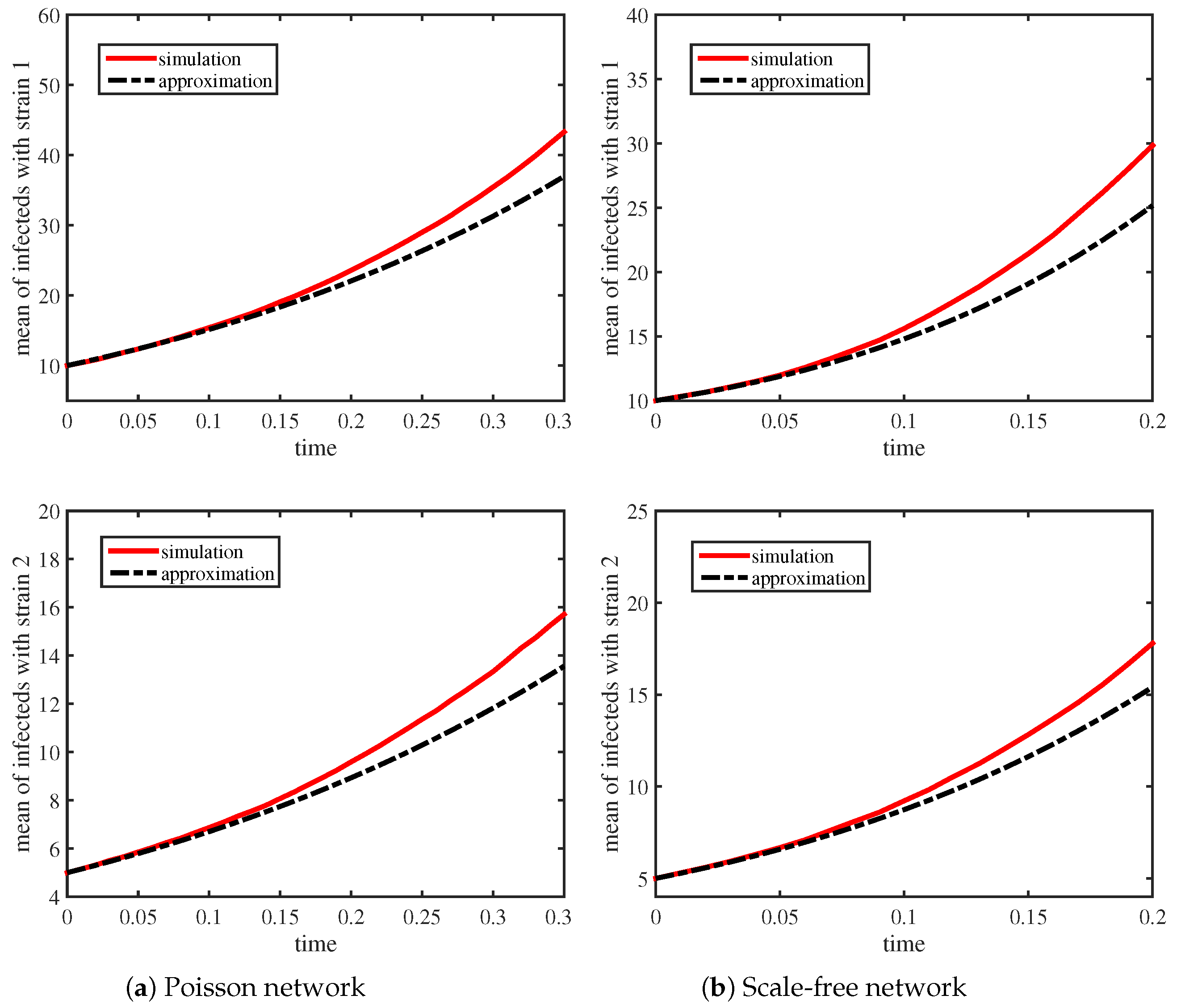
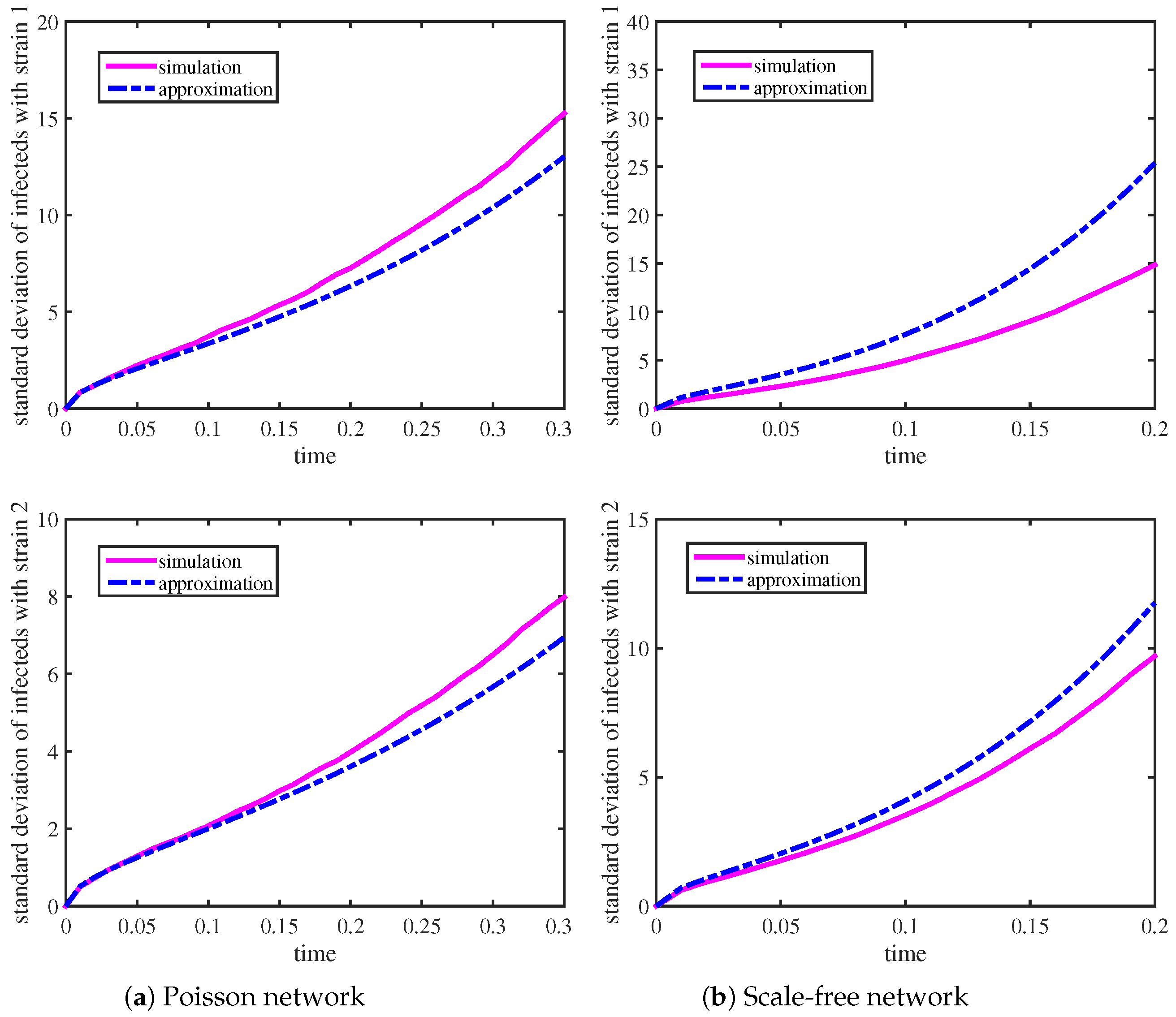
$r_2$	3.0193	7.0476

lists the parameter values of Figure 1 and Figure 2.

Figure 1 and Figure 2 show the results of the stochastic simulations compared with the theoretical predictions. Figure 1 shows that the means of the infected individuals with strain 1 and strain 2 for the two networks. The red solid lines are obtained based on 1000 simulations, and the black dashed lines are obtained by using (7). We can see that the means of the infected individuals with strain 1 and strain 2 in the stochastic simulations are consistent with the predicted results in the early growth stage. Specifically, we find that the growth rates $r_1$ and $r_2$ for the Scale-free network are larger than that for the Poisson network. Although the average degrees of these two networks are the same, Scale-free networks have a greater variance and skewness. This is the reason for the difference.

We show the temporal evolution of the standard deviation of the infected individuals with strain 1 and strain 2 in Figure 2. The pink solid lines are obtained based on simulations, and the blue dashed lines are obtained by using (12) and (13). Figure 2 shows the period of time at which we have agreement in the standard deviations of those infected with strain 1 and strain 2 between the two networks with the predicted results. From Table 1, we speculate that the network with lower variance and skewness has a stabilizing effect during the exponential growth phase; that is to say, those infected in the network with high heterogeneity always display greater variation about the mean.

5. Conclusions

We have considered the spread of SIR-type two-strain infections in heterogeneous networks. We focus on the variance of the prevalence of the infection. Using the result of Kurtz [21] enables us to analyze the stochastic dynamic of the disease using the deterministic limiting system. Furthermore, inspired by Graham and Volz et al. [18,22], we reduce a relatively low dimensional deterministic network-based epidemic model by using the probability generating function. Then, expressions for the asymptotic variances of those infected with strain 1 and strain 2 during the early growth are obtained. This result provides support for us to understand the early behavior of infectious disease with two strains. For the numerical scheme, the theoretical results are used to improve the efficiency of the calculation.

By comparing the results that are derived analytically with stochastic simulations, we demonstrate that the approximate performance of the mean and standard deviation of the number of those infected with strain 1 and strain 2 for the SIR epidemic process in the Poisson network and the Scale-free network. We can get a strong agreement between the results and simulations, as can be seen in Figure 1 and Figure 2. Furthermore, we show that the network with lower variance and skewness has a stabilizing effect during the exponential growth phase; that is to say, those infected in the network with high heterogeneity always display greater variation about the mean. An implication of this result is that, in the situation of an outbreak of a disease, if we are able to target the very well-connected people in the network, then we can decrease the spread of the disease in the population efficiently.

Of course, we only study the simple scenario of the two-strain SIR epidemic spreading in heterogeneous networks. For mutation, cross-infection, and other forms of interrelationship between strains, we can do further research. In summary, our work provides some insights into the stochastic dynamics of infectious diseases with two strains.

References

1. Kermack, W.O.; Mckendrick, A.G. A contribution to the mathematical theory of epidemics. Proc. R. Soc. Lond. A 1927, 115, 700–721. [Google Scholar]
2. Albert, R.; Barabasi, A.L. Statistical mechanics of complex networks. Rev. Mod. Phys. 2001, 74, 47–97. [Google Scholar] [CrossRef]
3. Pan, W.; Sun, G.Q.; Jin, Z. How demography-driven evolving networks impact epidemic transmission between communities. J. Theor. Biol. 2015, 382, 309–319. [Google Scholar] [CrossRef]
4. Li, B.; Eskandari, Z. Dynamical analysis of a discrete-time SIR epidemic model. J. Frankl. Inst.-Eng. Appl. Math. 2023, 360, 7989–8007. [Google Scholar] [CrossRef]
5. Maleki, M.; Mahmoudi, M.R.; Wraith, D.; Pho, K.H. Time series modelling to forecast the confirmed and recovered cases of COVID-19. Travel Med. Infect. Dis. 2020, 37, 101742. [Google Scholar] [CrossRef] [PubMed]
6. Mahmoudi, M.R.; Heydari, M.H.; Qasem, S.N.; Mosavi, A.; Band, S.S. Principal component analysis to study the relations between the spread rates of COVID-19 in high risks countries. Alex. Eng. J. 2021, 60, 457–464. [Google Scholar] [CrossRef]
7. Li, X.Z.; Duan, X.C.; Ghosh, M.; Ruan, X.Y. Pathogen coexistence induced by saturating contact rates. Nonlinear Anal.-Real World Appl. 2009, 10, 3298–3311. [Google Scholar] [CrossRef]
8. Chen, C.; Kang, Y.M. Dynamics of a stochastic multi-strain sis epidemic model driven by lévy noise. Commun. Nonlinear Sci. Numer. Simul. 2017, 42, 379–395. [Google Scholar] [CrossRef]
9. Zhang, H.F.; Shu, P.P.; Wang, Z.; Tang, M.; Small, M. Preferential imitation can invalidate targeted subsidy policies on seasonal-influenza diseases. Appl. Math. Comput. 2017, 294, 332–342. [Google Scholar] [CrossRef]
10. Ackleh, A.S.; Allen, L.J.S. Competitive exclusion and coexistence for pathogens in an epidemic model with variable population size. J. Math. Biol. 2003, 47, 153–168. [Google Scholar] [CrossRef]
11. Newman, M.E.J. The structure and function of complex networks. SIAM Rev. 2003, 45, 167–256. [Google Scholar] [CrossRef]
12. Taylor, M.; Taylor, T.J.; Kiss, I.Z. Epidemic threshold and control in a dynamic network. Phys. Rev. E 2012, 85, 016103. [Google Scholar] [CrossRef] [PubMed]
13. Ma, J.L.; van den Driessche, P.; Willeboordse, F.H. Effective degree household network disease model. J. Math. Biol. 2013, 66, 75–94. [Google Scholar] [CrossRef] [PubMed]
14. Naik, P.A.; Eskandari, Z. Nonlinear dynamics of a three-dimensional discrete-time delay neural network. Int. J. Biomath. 2023, in press. [CrossRef]
15. Karrer, B.; Newman, M.E.J. Competing epidemics on complex networks. Phys. Rev. E 2011, 84, 036106. [Google Scholar] [CrossRef] [PubMed]
16. Yao, Y.; Zhang, J. A two-strain epidemic model on complex networks with demographics. J. Biol. Syst. 2016, 24, 577–609. [Google Scholar] [CrossRef]
17. Chung, K.W.; Lui, R. Dynamics of two-strain influenza model with cross-immunity and no quarantine class. J. Math. Biol. 2016, 73, 1467–1489. [Google Scholar] [CrossRef]
18. Graham, M.; House, T. Dynamics of stochastic epidemics on heterogeneous networks. J. Math. Biol. 2014, 68, 1583–1605. [Google Scholar] [CrossRef]
19. Allen, L.J.S. A primer on stochastic epidemic models: Formulation, numerical simulation, and analysis. Infect. Dis. Model. 2017, 2, 128–142. [Google Scholar] [CrossRef]
20. El Hajji, M.; Sayari, S.; Zaghdani, A. Mathematical analysis of an “SIR” epidemic model in a continuous reactor-deterministic and probabilistic approaches. J. Korean Math. Soc. 2021, 58, 45–67. [Google Scholar]
21. Ethier, S.N.; Kurtz, T.G. Markov Processes: Characterization and Convergence; John Wiley & Sons, Inc.: Hoboken, NJ, USA, 1986; pp. 452–459. [Google Scholar]
22. Volz, E. SIR dynamics in random networks with heterogeneous connectivity. J. Math. Biol. 2008, 56, 293–310. [Google Scholar] [CrossRef] [PubMed]
Figure 1. Demonstration of the mean early growth behaviour of the number of those infected with strain 1 and strain 2 for Poisson and Scale-free networks.
Symmetry 15 01813 g001
Figure 2. Demonstration of the standard deviation of the number of those infected with strain 1 and strain 2 for Poisson and Scale-free networks.
Symmetry 15 01813 g002