Investigation of Fractional Nonlinear Regularized Long-Wave Models via Novel Techniques

Abstract

The main goal of the current work is to develop numerical approaches that use the Yang transform, the homotopy perturbation method (HPM), and the Adomian decomposition method to analyze the fractional model of the regularized long-wave equation. The shallow-water waves and ion-acoustic waves in plasma are both explained by the regularized long-wave equation. The first method combines the Yang transform with the homotopy perturbation method and He’s polynomials. In contrast, the second method combines the Yang transform with the Adomian polynomials and the decomposition method. The Caputo sense is applied to the fractional derivatives. The strategy’s effectiveness is shown by providing a variety of fractional and integer-order graphs and tables. To confirm the validity of each result, the technique was substituted into the equation. The described methods can be used to find the solutions to these kinds of equations as infinite series, and when these series are in closed form, they give the precise solution. The results support the claim that this approach is simple, strong, and efficient for obtaining exact solutions for nonlinear fractional differential equations. The method is a strong contender to contribute to the existing literature.

1. Introduction

As far back as the classical integer order analysis goes, fractional-order calculus studies have a long history. However, have not been utilized in the physical sciences for a long time. Furthermore, over the past few decades, applications of fractional calculus in applied mathematics, control [1], viscoelasticity [2], electromagnetic [3], and electrochemistry [4] have grown in popularity. The advancement of symbolic computation software has further aided this growth. Fractional derivatives and integrals can be used to represent a variety of multidisciplinary applications. Some basic explanations and applications of fractional calculus are provided in [5,6]. In [7], the existence and distinctiveness of the solutions are also explored. Fractional derivatives and integrals have recently received new definitions from several scientists and engineers, who have utilized them to describe a variety of physical phenomena. In a study, Vazquez [8] provided a brief, non-exhaustive, comprehensive overview of the mathematical tool connected to fractional-order derivatives and integrals, along with an interpretation of various domains where they are either are being used or may one day be used. The existence, uniqueness, and regularity of solutions to the heat equation of the arbitrary order were investigated by Bonfortea et al. in a research study [9]. Excellent research on differential equations of fractional-order derivatives and their uses in bioengineering may be found in a monograph by Magin [10]. Magin [11] carried out ground-breaking research on fractional calculus-based mathematical models of complicated dynamics in biological tissues.

In recent years, a growing number of issues in biology, chemistry, engineering, physics, economics, and other application areas have been modelled using fractional differential equations [12,13,14]. The fractional differential equation is a helpful tool for representing nonlinear events in scientific and engineering models. In applied mathematics and engineering, partial differential equations, particularly nonlinear ones, have been utilized to simulate a wide range of scientific phenomena [15,16,17]. Fractional-order partial differential equations (FPDEs) allowed researchers to recognize and model a wide range of significant and real-world physical issues in parallel with their work in the physical sciences [18,19,20]. It has always been claimed how important it is to obtain approximations for them using either numerical or analytical methods [21,22,23]. As a result, symmetry analysis is an excellent tool for understanding partial differential equations, particularly when looking at equations derived from mathematical ideas related to accounting. Despite the idea that symmetry is the basis of nature, symmetry is absent from “most” observations of the natural world. Creating unexpected symmetry-breaking events is a creative way to mask symmetry. The two types of symmetry are finite and infinitesimal. Discrete and continuous finite symmetries come in two different varieties. Parity and temporal inversion are examples of natural symmetries that are “discrete”, whereas space is a continuous change. Patterns have always captivated mathematicians. The classification of spatial and planar patterns took off in the seventeenth century [24,25]. Regrettably, the precise solution of fractional nonlinear differential equations has been shown to be exceedingly challenging. Many researchers have developed a range of methods to examine the solutions of nonlinear partial differential equations since the early 2000s, such as the Elzaki transform decomposition method for time-fractional Swift–Hohenberg equations [26] and Navier–Stokes equations [27], the natural decomposition method for nonlinear conformable time-fractional Boussinesq equations [28] and conformable time-fractional Cahn–Hilliard equations [29], the homotopy perturbation method for the Noyes–Field model of the time-fractional Belousov–Zhabotinsky reaction [30] and time-fractional Fisher’s equation [31], the first integral method for the modified Benjamin–Bona–Mahony equation [32] and Burgers–Korteweg–de Vries equation [33], the $\frac{G^{\prime }}{G}$ expansion method for the conformable fractional Nizhnik–Novikov–Veselov system [34] and time-fractional Kaup–Kupershmidt equation [35], and many more [36,37,38,39,40,41,42].

To analyze dispersive water-wave models, Peregrine introduced the RLW equation in 1966 [43]. This work considers two alternative fractional homogeneous nonlinear regularized long-wave (RLW) equations. There are various specialized RLWs in the literature. According to some researchers, the RLW equations are superior to the traditional Korteweg–de Vries (KdV) equation [44,45]. We use the traditional Caputo operator in combination with the Yang transform decomposition method (YTDM) and the Homotopy Perturbation Yang Transform Method (HPTM) to solve two unique RLW problems. The Yang transform (YT), which Xiao-Jun Yang introduced, can be used to resolve a variety of differential equations with constant coefficients. Adomian proposed the Adomian decomposition method in 1980 [46], which is a useful technique for generating a numerical and explicit solution to a set of differential equations that reflect a physical problem. Ji Huan He is credited with developing the homotopy perturbation method (HPM) [47]. In recent years, many scientists have employed the HPM to resolve many forms of differential equations, both linear and nonlinear. After that, we discover their approximations and examine the numerical simulations of the results. The nonlinear RLW equations are provided by [48,49].

$$D_{\vartheta }^{\wp }\mathbb{U}(\mathfrak{y},\vartheta )-{\mathbb{U}}_{\mathfrak{y}\mathfrak{y}\vartheta }(\mathfrak{y},\vartheta )+{\left(\frac{{\mathbb{U}}^2(\mathfrak{y},\vartheta )}{2}\right)}_{\mathfrak{y}}=0,0<\wp \le 1,$$

(1)

which has the initial condition

$$\mathbb{U}(\mathfrak{y},0)=\mathfrak{y}.$$

and

$$D_{\vartheta }^{\wp }\mathbb{U}(\mathfrak{y},\vartheta )+{\mathbb{U}}_{\mathfrak{y}}(\mathfrak{y},\vartheta )-{\mathbb{U}}_{\mathfrak{y}\mathfrak{y}}(\mathfrak{y},\vartheta )+{\mathbb{U}}^2(\mathfrak{y},\vartheta ){\mathbb{U}}_{\mathfrak{y}}(\mathfrak{y},\vartheta )+\frac{1}{6}{\left[e^{(-2\mathfrak{y}+4\vartheta )}{\mathbb{U}}_{\mathfrak{y}\vartheta }(\mathfrak{y},\vartheta )\right]}_{\mathfrak{y}}=0,0<\wp \le 1,$$

(2)

which has the initial condition

$$\mathbb{U}(\mathfrak{y},0)=e^{-\mathfrak{y}}.$$

where $(\mathfrak{y},\vartheta )\in \mathbf{R}\times [0,T],0<\wp \le 1,$ and $D_{\vartheta }^{\wp }$ represents the classical Caputo operator of order ℘.

Dealing with fractional-order systems is necessary because they have complicated behavioral patterns of physical systems called memory and hereditary features, which provide a more realistic way to describe nonlinear regularized long-wave models. The memory attribute of the fractional-order models enables the incorporation of more historical data, improving prediction and model translation. The hereditary property also describes the genetic profile along with age and the immune-system condition. Fractional-order calculus has a wide range of applications in modelling dynamical processes in many well-known domains due to these qualities. On the other hand, the literature has exhaustively examined the physical structures and illustrative applications of such problems. The nonlinear RLW equation’s ability to accurately describe a variety of significant physical phenomena, including ion-acoustic plasma and shallow-water waves, is essential in studying nonlinear dispersive waves. Numerous scholars have explored these models, particularly their fractional forms [50,51]. See Stoker and Waves [52] for further information on the RLW equation’s physical significance. Sanjay Kumar et al. simulate and study dark and bright soliton solutions of 1D and 2D regularized long-wave (RLW) models [53]. In [54], two numerical algorithms are designed for the simulation of the generalized regularized long-wave (GRLW) model via local radial basis functions (LRBFs) and Scale-3 Haar wavelets (S3HWs).

The structure of this work is as follows. This study is intended to give simple definitions and properties of fractional calculus in Section 2. Section 3 and Section 4 present the suggested approaches, and Section 5 provides the convergence analysis of the proposed methods. Section 6 describes how to use these approaches to solve various cases. In Section 7, we conclude the paper with the key findings.

2. Preliminaries

This section is concerned with the fundamental concept of fractional calculus along with Yang transform theory.

2.1. Definition

The fractional Caputo derivative is given as [55,56]

$$\begin{array}{cc}\hfill & D_{\vartheta }^{\wp }\mathbb{U}(\mathfrak{y},\vartheta )=\frac{1}{\mathrm{\Gamma }(k-\wp )}{\int }_0^{\vartheta }{(\vartheta -\wp )}^{k-\wp -1}{\mathbb{U}}^{\left(k\right)}(\mathfrak{y},\wp )d\wp ,k-1<\wp \le k,k\in \mathbf{N}.\hfill \end{array}$$

(3)

2.2. Definition

The Yang transform is stated as [57,58]

$$Y\left\{\mathbb{U}\left(\vartheta \right)\right\}=M\left(u\right)={\int }_0^{\infty }{e}^{\frac{-\vartheta }{u}}\mathbb{U}\left(\vartheta \right)d\vartheta ,\vartheta >0,u\in (-{\vartheta }_1,{\vartheta }_2),$$

(4)

and the inverse Yang transform is stated as

$$Y^{-1}\left\{M\left(u\right)\right\}=\mathbb{U}\left(\vartheta \right).$$

(5)

2.3. Definition

The nth derivative Yang transform is stated as [57,58]

$$Y\left\{{\mathbb{U}}^n\left(\vartheta \right)\right\}=\frac{M\left(u\right)}{u^n}-\sum _{k=0}^{n-1}\frac{{\mathbb{U}}^k\left(0\right)}{u^{n-k-1}},\forall n=1,2,3,\cdots$$

(6)

2.4. Definition

The Yang transform in connection with the fractional-order derivative is stated as [57,58]

$$Y\left\{{\mathbb{U}}^{\wp }\left(\vartheta \right)\right\}=\frac{M\left(u\right)}{u^{\wp }}-\sum _{k=0}^{n-1}\frac{{\mathbb{U}}^k\left(0\right)}{u^{\wp -(k+1)}},0<\wp \le n.$$

(7)

3. General Implementation of the HPTM

In this section, we describe the main steps of the HPTM for finding the exact solution of FPDEs.

$$D_{\vartheta }^{\wp }\mathbb{U}(\mathfrak{y},\vartheta )={\mathcal{P}}_1\left[\mathfrak{y}\right]\mathbb{U}(\mathfrak{y},\vartheta )+{\mathcal{Q}}_1\left[\mathfrak{y}\right]\mathbb{U}(\mathfrak{y},\vartheta ),0<\wp \le 1,$$

(8)

subjected to initial conditions

$$\mathbb{U}(\mathfrak{y},0)=\xi \left(\mathfrak{y}\right).$$

Here, $D_{\vartheta }^{\wp }=\frac{{\partial }^{\wp }}{\partial {\vartheta }^{\wp }}$ represents the Caputo operator, and ${\mathcal{P}}_1\left[\mathfrak{y}\right],$${\mathcal{Q}}_1\left[\mathfrak{y}\right]$ are linear and nonlinear terms.

By applying the Yang transform, we have

$$Y\left[D_{\vartheta }^{\wp }\mathbb{U}(\mathfrak{y},\vartheta )\right]=Y[{\mathcal{P}}_1\left[\mathfrak{y}\right]\mathbb{U}(\mathfrak{y},\vartheta )+{\mathcal{Q}}_1\left[\mathfrak{y}\right]\mathbb{U}(\mathfrak{y},\vartheta )],$$

(9)

$$\frac{1}{u^{\wp }}\{M\left(u\right)-u\mathbb{U}\left(0\right)\}=Y[{\mathcal{P}}_1\left[\mathfrak{y}\right]\mathbb{U}(\mathfrak{y},\vartheta )+{\mathcal{Q}}_1\left[\mathfrak{y}\right]\mathbb{U}(\mathfrak{y},\vartheta )].$$

(10)

After simplifying, we have

$$M\left(\mathbb{U}\right)=u\mathbb{U}\left(0\right)+u^{\wp }Y[{\mathcal{P}}_1\left[\mathfrak{y}\right]\mathbb{U}(\mathfrak{y},\vartheta )+{\mathcal{Q}}_1\left[\mathfrak{y}\right]\mathbb{U}(\mathfrak{y},\vartheta )].$$

(11)

By applying the inverse Yang transform, we have

$$\mathbb{U}(\mathfrak{y},\vartheta )=\mathbb{U}\left(0\right)+Y^{-1}\left[u^{\wp }Y[{\mathcal{P}}_1\left[\mathfrak{y}\right]\mathbb{U}(\mathfrak{y},\vartheta )+{\mathcal{Q}}_1\left[\mathfrak{y}\right]\mathbb{U}(\mathfrak{y},\vartheta )]\right].$$

(12)

Now, by HPM

$$\mathbb{U}(\mathfrak{y},\vartheta )=\sum _{k=0}^{\infty }{ϵ}^k{\mathbb{U}}_k(\mathfrak{y},\vartheta ).$$

(13)

with parameter $ϵ\in [0,1]$.

The nonlinear term is taken as

$${\mathcal{Q}}_1\left[\mathfrak{y}\right]\mathbb{U}(\mathfrak{y},\vartheta )=\sum _{k=0}^{\infty }{ϵ}^k{H}_n\left(\mathbb{U}\right).$$

(14)

Additionally, He’s polynomials $H_k\left(\mathbb{U}\right)$ are taken as

$$H_n({\mathbb{U}}_0,{\mathbb{U}}_1,...,{\mathbb{U}}_n)=\frac{1}{\mathrm{\Gamma }(n+1)}{D}_{ϵ}^k{\left[{\mathcal{Q}}_1\left(\sum _{k=0}^{\infty }{ϵ}^i{\mathbb{U}}_i\right)\right]}_{ϵ=0},$$

(15)

where $D_{ϵ}^k=\frac{{\partial }^k}{\partial {ϵ}^k}.$

By putting (14) and (15) in (12), we obtain

$$\sum _{k=0}^{\infty }{ϵ}^k{\mathbb{U}}_k(\mathfrak{y},\vartheta )=\mathbb{U}\left(0\right)+ϵ\times \left(Y^{-1}\left[u^{\wp }Y\{{\mathcal{P}}_1\sum _{k=0}^{\infty }{ϵ}^k{\mathbb{U}}_k(\mathfrak{y},\vartheta )+\sum _{k=0}^{\infty }{ϵ}^k{H}_k\left(\mathbb{U}\right)\}\right]\right).$$

(16)

By comparison with the $ϵ$ coefficient, we obtain

$$\begin{array}{cc}\hfill & {ϵ}^0:{\mathbb{U}}_0(\mathfrak{y},\vartheta )=\mathbb{U}\left(0\right),\hfill \\ \hfill & {ϵ}^1:{\mathbb{U}}_1(\mathfrak{y},\vartheta )=Y^{-1}\left[u^{\wp }Y({\mathcal{P}}_1\left[\mathfrak{y}\right]{\mathbb{U}}_0(\mathfrak{y},\vartheta )+H_0\left(\mathbb{U}\right))\right],\hfill \\ \hfill & {ϵ}^2:{\mathbb{U}}_2(\mathfrak{y},\vartheta )=Y^{-1}\left[u^{\wp }Y({\mathcal{P}}_1\left[\mathfrak{y}\right]{\mathbb{U}}_1(\mathfrak{y},\vartheta )+H_1\left(\mathbb{U}\right))\right],\hfill \\ \hfill & .\hfill \\ \hfill & .\hfill \\ \hfill & .\hfill \\ \hfill & {ϵ}^k:{\mathbb{U}}_k(\mathfrak{y},\vartheta )=Y^{-1}\left[u^{\wp }Y({\mathcal{P}}_1\left[\mathfrak{y}\right]{\mathbb{U}}_{k-1}(\mathfrak{y},\vartheta )+H_{k-1}\left(\mathbb{U}\right))\right],\hfill \\ \hfill k>0,k\in \mathbf{N}.\hfill \end{array}$$

(17)

Lastly, the ${\mathbb{U}}_k(\mathfrak{y},\vartheta )$ solution is calculated as

$$\mathbb{U}(\mathfrak{y},\vartheta )=\underset{M\to \infty }{lim}\sum _{k=1}^M{\mathbb{U}}_k(\mathfrak{y},\vartheta ).$$

(18)

4. General Implementation of the YTDM

In this section, we describe the main steps of the YTDM for finding the exact solution of FPDEs.

$$D_{\vartheta }^{\wp }\mathbb{U}(\mathfrak{y},\vartheta )={\mathcal{P}}_1(\mathfrak{y},\vartheta )+{\mathcal{Q}}_1(\mathfrak{y},\vartheta ),0<\wp \le 1,$$

(19)

subjected to initial conditions

$$\mathbb{U}(\mathfrak{y},0)=\xi \left(\mathfrak{y}\right).$$

Here, $D_{\vartheta }^{\wp }=\frac{{\partial }^{\wp }}{\partial {\vartheta }^{\wp }}$ represents the Caputo operator, and ${\mathcal{P}}_1$ and ${\mathcal{Q}}_1$ are linear and non-linear terms. By applying the Yang transform, we have

$$\begin{array}{cc}\hfill & Y\left[D_{\vartheta }^{\wp }\mathbb{U}(\mathfrak{y},\vartheta )\right]=Y[{\mathcal{P}}_1(\mathfrak{y},\vartheta )+{\mathcal{Q}}_1(\mathfrak{y},\vartheta )],\hfill \\ \hfill & \frac{1}{u^{\wp }}\{M\left(u\right)-u\mathbb{U}\left(0\right)\}=Y[{\mathcal{P}}_1(\mathfrak{y},\vartheta )+{\mathcal{Q}}_1(\mathfrak{y},\vartheta )].\hfill \end{array}$$

(20)

After simplifying, we have

$$M\left(\mathbb{U}\right)=u\mathbb{U}\left(0\right)+u^{\wp }Y[{\mathcal{P}}_1(\mathfrak{y},\vartheta )+{\mathcal{Q}}_1(\mathfrak{y},\vartheta )],$$

(21)

By applying the inverse Yang transform, we have

$$\mathbb{U}(\mathfrak{y},\vartheta )=\mathbb{U}\left(0\right)+Y^{-1}[u^{\wp }Y[{\mathcal{P}}_1(\mathfrak{y},\vartheta )+{\mathcal{Q}}_1(\mathfrak{y},\vartheta )].$$

(22)

Now, by YTDM

$$\mathbb{U}(\mathfrak{y},\vartheta )=\sum _{m=0}^{\infty }{\mathbb{U}}_m(\mathfrak{y},\vartheta ).$$

(23)

The nonlinear term is taken as

$${\mathcal{Q}}_1(\mathfrak{y},\vartheta )=\sum _{m=0}^{\infty }{\mathcal{A}}_m.$$

(24)

with

$${\mathcal{A}}_m=\frac{1}{m!}{\left[\frac{{\partial }^m}{\partial {\ell }^m}\left\{{\mathcal{Q}}_1\left(\sum _{k=0}^{\infty }{\ell }^k{\mathfrak{y}}_k,\sum _{k=0}^{\infty }{\ell }^k{\vartheta }_k\right)\right\}\right]}_{\ell =0},$$

(25)

By putting (24) and (26) into (23), we obtain

$$\sum _{m=0}^{\infty }{\mathbb{U}}_m(\mathfrak{y},\vartheta )=\mathbb{U}\left(0\right)+Y^{-1}{u}^{\wp }\left[Y\left\{{\mathcal{P}}_1(\sum _{m=0}^{\infty }{\mathfrak{y}}_m,\sum _{m=0}^{\infty }{\vartheta }_m)+\sum _{m=0}^{\infty }{\mathcal{A}}_m\right\}\right].$$

(26)

So, we can write

$${\mathbb{U}}_0(\mathfrak{y},\vartheta )=\mathbb{U}\left(0\right),$$

(27)

$${\mathbb{U}}_1(\mathfrak{y},\vartheta )=Y^{-1}\left[u^{\wp }Y\{{\mathcal{P}}_1({\mathfrak{y}}_0,{\vartheta }_0)+{\mathcal{A}}_0\}\right],$$

Hence, in general for $m\ge 1$, we obtain

$${\mathbb{U}}_{m+1}(\mathfrak{y},\vartheta )=Y^{-1}\left[u^{\wp }Y\{{\mathcal{P}}_1({\mathfrak{y}}_m,{\vartheta }_m)+{\mathcal{A}}_m\}\right].$$

5. Convergence Analysis

Here, we discuss the convergence analysis of the proposed methods.

Theorem 1.

Let us assume that $\mathbb{U}$ and ${\mathbb{U}}_n(\mathfrak{y},\vartheta )$ are defined in Banach space. If this is the case, the series solution described by Equation (14) converges to the solution of Equation (8) if $\exists \eta \in (0,1)$ such that $\left|\right|{\mathbb{U}}_{n+1}\left|\right|\le \eta \left|\right|{\mathbb{U}}_n\left|\right|$, so the convergence condition has been demonstrated [59].

Theorem 2.

The non-linear operator $M\left(\mathbb{U}\right)$ expressed by (24) satisfies the Lipschitz condition $\left|\right|M\left(\mathcal{Q}\right)-M\left({\mathcal{Q}}^{*}\right)\left|\right|\le \delta \left|\right|\mathcal{Q}-{\mathcal{Q}}^{*}\left|\right|$; using the Lipschitz constant $\delta ,0\le \delta <1$, for any $\mathcal{Q},{\mathcal{Q}}^{*}\in C[0,1]$, the sequence leads to the precise solution $\mathbb{U}$ if $\left|\right|a_0\left|\right|<\infty$. Proof: Check [60].

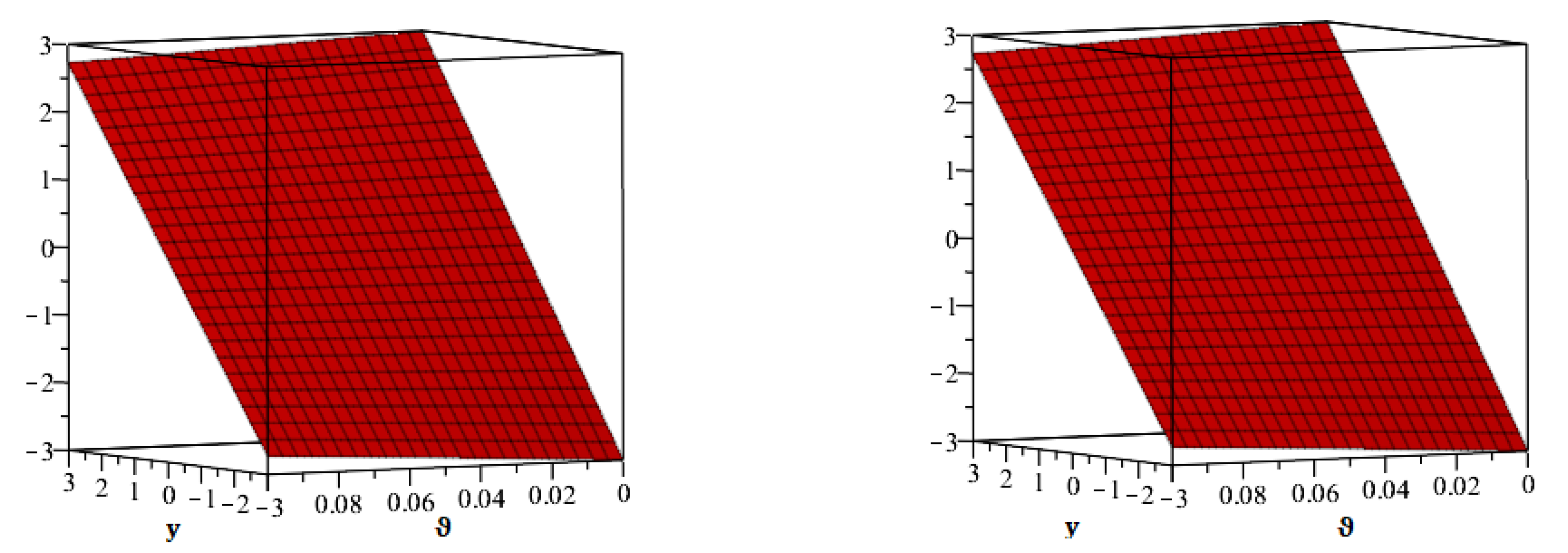
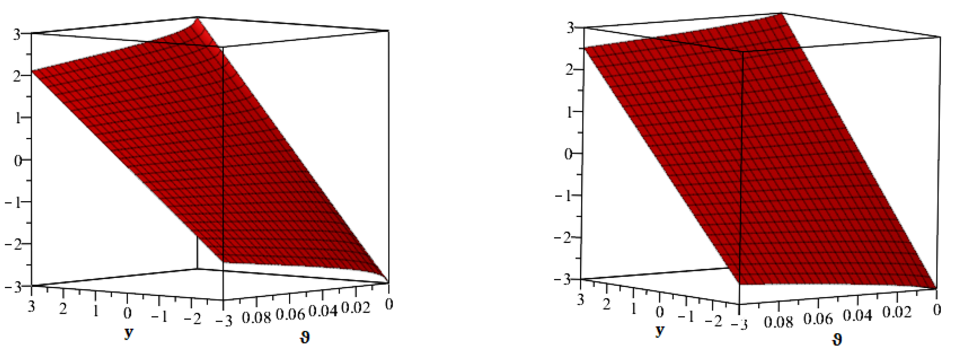
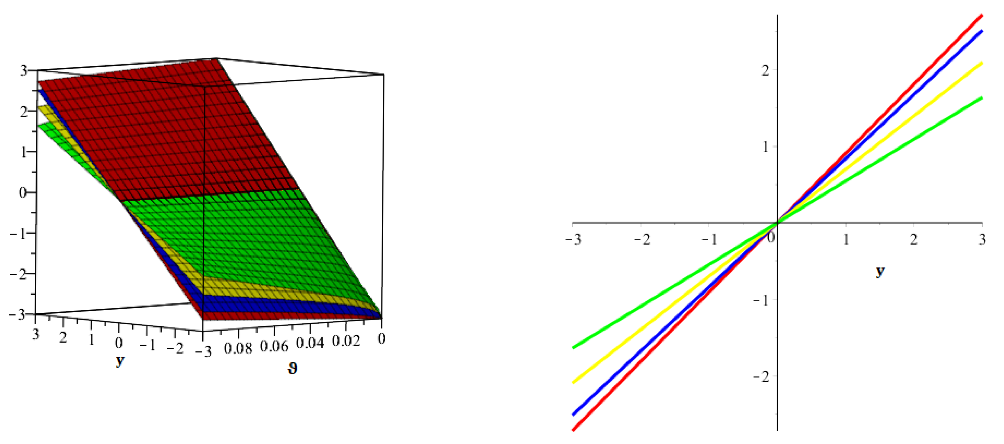
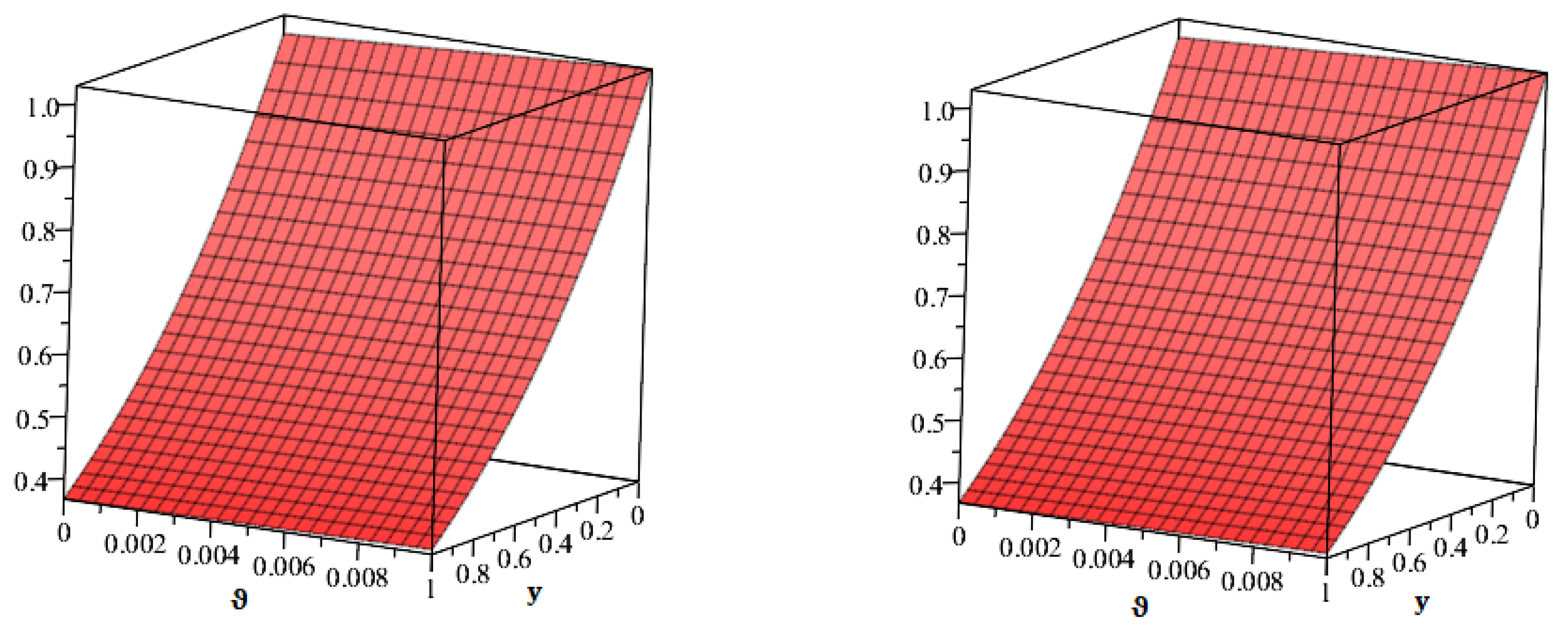
6. Numerical Examples

In this part, we will implement the proposed methods to solve nonlinear fractional RLW equations.

Example 1.

Assume nonlinear fractional RLW equation of the form

$$D_{\vartheta }^{\wp }\mathbb{U}(\mathfrak{y},\vartheta )-{\mathbb{U}}_{\mathfrak{y}\mathfrak{y}\vartheta }(\mathfrak{y},\vartheta )+{\left(\frac{{\mathbb{U}}^2(\mathfrak{y},\vartheta )}{2}\right)}_{\mathfrak{y}}=0,0<\wp \le 1,$$

(28)

subjected to initial condition

$$\mathbb{U}(\mathfrak{y},0)=\mathfrak{y}.$$

By applying the Yang transform, we have

$$Y\left(\frac{{\partial }^{\wp }\mathbb{U}}{\partial {\vartheta }^{\wp }}\right)=Y\left({\mathbb{U}}_{\mathfrak{y}\mathfrak{y}\vartheta }(\mathfrak{y},\vartheta )-{\left(\frac{{\mathbb{U}}^2(\mathfrak{y},\vartheta )}{2}\right)}_{\mathfrak{y}}\right),$$

(29)

By means of the Yang differentiation property, we obtain

$$\frac{1}{u^{\wp }}\{M\left(u\right)-u\mathbb{U}\left(0\right)\}=Y\left({\mathbb{U}}_{\mathfrak{y}\mathfrak{y}\vartheta }(\mathfrak{y},\vartheta )-{\left(\frac{{\mathbb{U}}^2(\mathfrak{y},\vartheta )}{2}\right)}_{\mathfrak{y}}\right),$$

(30)

$$M\left(u\right)=u\mathbb{U}\left(0\right)+u^{\wp }Y\left({\mathbb{U}}_{\mathfrak{y}\mathfrak{y}\vartheta }(\mathfrak{y},\vartheta )-{\left(\frac{{\mathbb{U}}^2(\mathfrak{y},\vartheta )}{2}\right)}_{\mathfrak{y}}\right).$$

(31)

By applying the inverse Yang transform, we have

$$\begin{array}{cc}\hfill & \mathbb{U}(\mathfrak{y},\vartheta )=\mathbb{U}\left(0\right)+Y^{-1}\left[u^{\wp }\left\{Y\left({\mathbb{U}}_{\mathfrak{y}\mathfrak{y}\vartheta }(\mathfrak{y},\vartheta )-{\left(\frac{{\mathbb{U}}^2(\mathfrak{y},\vartheta )}{2}\right)}_{\mathfrak{y}}\right)\right\}\right],\hfill \\ \hfill & \mathbb{U}(\mathfrak{y},\vartheta )=\mathfrak{y}+Y^{-1}\left[u^{\wp }\left\{Y\left({\mathbb{U}}_{\mathfrak{y}\mathfrak{y}\vartheta }(\mathfrak{y},\vartheta )-{\left(\frac{{\mathbb{U}}^2(\mathfrak{y},\vartheta )}{2}\right)}_{\mathfrak{y}}\right)\right\}\right].\hfill \end{array}$$

(32)

Now by HPM

$$\sum _{k=0}^{\infty }{ϵ}^k{\mathbb{U}}_k(\mathfrak{y},\vartheta )=\mathfrak{y}+ϵ\left(Y^{-1}\left[u^{\wp }Y\left[{\left(\sum _{k=0}^{\infty }{ϵ}^k{\mathbb{U}}_k(\mathfrak{y},\vartheta )\right)}_{\mathfrak{y}\mathfrak{y}\vartheta }-\left(\sum _{k=0}^{\infty }{ϵ}^k{H}_k\left(\mathbb{U}\right)\right)\right]\right]\right).$$

(33)

Additionally, He’s polynomial $H_k\left(\mathbb{U}\right)$ is utilized to determine non-linear terms as

$$\sum _{k=0}^{\infty }{ϵ}^k{H}_k\left(\mathbb{U}\right)={\left(\frac{{\mathbb{U}}^2(\mathfrak{y},\vartheta )}{2}\right)}_{\mathfrak{y}}$$

(34)

Few terms of He’s polynomials are calculated as

$$\begin{array}{cc}\hfill & H_0\left(\mathbb{U}\right)={\mathbb{U}}_0{\left({\mathbb{U}}_0\right)}_{\mathfrak{y}},\hfill \\ \hfill & H_1\left(\mathbb{U}\right)={\mathbb{U}}_0{\left({\mathbb{U}}_1\right)}_{\mathfrak{y}}+{\mathbb{U}}_1{\left({\mathbb{U}}_0\right)}_{\mathfrak{y}}\hfill \\ \hfill & H_2\left(\mathbb{U}\right)={\mathbb{U}}_0{\left({\mathbb{U}}_2\right)}_{\mathfrak{y}}+{\mathbb{U}}_1{\left({\mathbb{U}}_1\right)}_{\mathfrak{y}}+{\mathbb{U}}_2{\left({\mathbb{U}}_0\right)}_{\mathfrak{y}}\hfill \end{array}$$

By comparison of ϵ coefficients, we obtain

$$\begin{array}{cc}\hfill & {ϵ}^0:{\mathbb{U}}_0(\mathfrak{y},\vartheta )=\mathfrak{y},\hfill \\ \hfill & {ϵ}^1:{\mathbb{U}}_1(\mathfrak{y},\vartheta )=Y^{-1}\left(u^{\wp }Y\left[{\left({\mathbb{U}}_0\right)}_{\mathfrak{y}\mathfrak{y}\vartheta }-H_0\left(\mathbb{U}\right)\right]\right)=-\mathfrak{y}\frac{{\vartheta }^{\wp }}{\Gamma (\wp +1)},\hfill \\ \hfill & {ϵ}^2:{\mathbb{U}}_2(\mathfrak{y},\vartheta )=Y^{-1}\left(u^{\wp }Y\left[{\left({\mathbb{U}}_1\right)}_{\mathfrak{y}\mathfrak{y}\vartheta }-H_1\left(\mathbb{U}\right)\right]\right)=2\mathfrak{y}\frac{{\vartheta }^{2\wp }}{\Gamma (2\wp +1)},\hfill \\ \hfill & {ϵ}^3:{\mathbb{U}}_3(\mathfrak{y},\vartheta )=Y^{-1}\left(u^{\wp }Y\left[{\left({\mathbb{U}}_2\right)}_{\mathfrak{y}\mathfrak{y}\vartheta }-H_2\left(\mathbb{U}\right)\right]\right)=-6\mathfrak{y}\frac{{\vartheta }^{3\wp }}{\Gamma (3\wp +1)},\hfill \\ \hfill & ⋮\hfill \end{array}$$

Lastly, the solution in series form is calculated as

$$\begin{array}{cc}\hfill & \mathbb{U}(\mathfrak{y},\vartheta )={\mathbb{U}}_0(\mathfrak{y},\vartheta )+{\mathbb{U}}_1(\mathfrak{y},\vartheta )+{\mathbb{U}}_2(\mathfrak{y},\vartheta )+\cdots \hfill \\ \hfill & \mathbb{U}(\mathfrak{y},\vartheta )=\mathfrak{y}-\mathfrak{y}\frac{{\vartheta }^{\wp }}{\Gamma (\wp +1)}+2\mathfrak{y}\frac{{\vartheta }^{2\wp }}{\Gamma (2\wp +1)}-6\mathfrak{y}\frac{{\vartheta }^{3\wp }}{\Gamma (3\wp +1)}+\cdots \hfill \end{array}$$

Considering the YTDM

By applying the Yang transform, we have

$$Y\left\{\frac{{\partial }^{\wp }\mathbb{U}}{\partial {\vartheta }^{\wp }}\right\}=Y\left({\mathbb{U}}_{\mathfrak{y}\mathfrak{y}\vartheta }(\mathfrak{y},\vartheta )-{\left(\frac{{\mathbb{U}}^2(\mathfrak{y},\vartheta )}{2}\right)}_{\mathfrak{y}}\right),$$

(35)

By means of Yang differentiation property, we obtain

$$\frac{1}{u^{\wp }}\{M\left(u\right)-u\mathbb{U}\left(0\right)\}=Y\left({\mathbb{U}}_{\mathfrak{y}\mathfrak{y}\vartheta }(\mathfrak{y},\vartheta )-{\left(\frac{{\mathbb{U}}^2(\mathfrak{y},\vartheta )}{2}\right)}_{\mathfrak{y}}\right),$$

(36)

$$M\left(u\right)=u\mathbb{U}\left(0\right)+u^{\wp }Y\left({\mathbb{U}}_{\mathfrak{y}\mathfrak{y}\vartheta }(\mathfrak{y},\vartheta )-{\left(\frac{{\mathbb{U}}^2(\mathfrak{y},\vartheta )}{2}\right)}_{\mathfrak{y}}\right).$$

(37)

By applying the inverse Yang transform, we have

$$\begin{array}{cc}\hfill & \mathbb{U}(\mathfrak{y},\vartheta )=\mathbb{U}\left(0\right)+Y^{-1}\left[u^{\wp }\left\{Y\left({\mathbb{U}}_{\mathfrak{y}\mathfrak{y}\vartheta }(\mathfrak{y},\vartheta )-{\left(\frac{{\mathbb{U}}^2(\mathfrak{y},\vartheta )}{2}\right)}_{\mathfrak{y}}\right)\right\}\right],\hfill \\ \hfill & \mathbb{U}(\mathfrak{y},\vartheta )=\frac{1}{{(1+{exp}^{\mathfrak{y}})}^2}+Y^{-1}\left[u^{\wp }\left\{Y\left({\mathbb{U}}_{\mathfrak{y}\mathfrak{y}\vartheta }(\mathfrak{y},\vartheta )-{\left(\frac{{\mathbb{U}}^2(\mathfrak{y},\vartheta )}{2}\right)}_{\mathfrak{y}}\right)\right\}\right].\hfill \end{array}$$

(38)

The series form solution is stated as

$$\mathbb{U}(\mathfrak{y},\vartheta )=\sum _{m=0}^{\infty }{\mathbb{U}}_m(\mathfrak{y},\vartheta ).$$

(39)

The nonlinear terms by Adomian polynomial sense are calculated as ${\left(\frac{{\mathbb{U}}^2(\mathfrak{y},\vartheta )}{2}\right)}_{\mathfrak{y}}={\sum }_{m=0}^{\infty }{\mathcal{A}}_m$. So, we obtain

$$\begin{array}{cc}\hfill & \sum _{m=0}^{\infty }{\mathbb{U}}_m(\mathfrak{y},\vartheta )=\mathbb{U}(\mathfrak{y},0)+Y^{-1}\left[u^{\wp }Y\left[{\mathbb{U}}_{\mathfrak{y}\mathfrak{y}\vartheta }(\mathfrak{y},\vartheta )-\sum _{m=0}^{\infty }{\mathcal{A}}_m\right]\right],\hfill \\ \hfill & \sum _{m=0}^{\infty }{\mathbb{U}}_m(\mathfrak{y},\vartheta )={(1-\mathfrak{y})}^{\left(\frac{1}{2}\right)}+Y^{-1}\left[u^{\wp }Y\left[{\mathbb{U}}_{\mathfrak{y}\mathfrak{y}\vartheta }(\mathfrak{y},\vartheta )-\sum _{m=0}^{\infty }{\mathcal{A}}_m\right]\right].\hfill \end{array}$$

(40)

The nonlinear terms are examined as,

$$\begin{array}{cc}\hfill & {\mathcal{A}}_0={\mathbb{U}}_0{\left({\mathbb{U}}_0\right)}_{\mathfrak{y}},\hfill \\ & {\mathcal{A}}_1={\mathbb{U}}_0{\left({\mathbb{U}}_1\right)}_{\mathfrak{y}}+{\mathbb{U}}_1{\left({\mathbb{U}}_0\right)}_{\mathfrak{y}},\hfill \\ & {\mathcal{A}}_2={\mathbb{U}}_0{\left({\mathbb{U}}_2\right)}_{\mathfrak{y}}+{\mathbb{U}}_1{\left({\mathbb{U}}_1\right)}_{\mathfrak{y}}+{\mathbb{U}}_2{\left({\mathbb{U}}_0\right)}_{\mathfrak{y}}.\hfill \end{array}$$

Now, by comparing both sides, we obtain

$${\mathbb{U}}_0(\mathfrak{y},\vartheta )=\mathfrak{y},$$

On $m=0$

$${\mathbb{U}}_1(\mathfrak{y},\vartheta )=-\mathfrak{y}\frac{{\vartheta }^{\wp }}{\mathrm{\Gamma }(\wp +1)},$$

On $m=1$

$$\begin{array}{cc}\hfill & {\mathbb{U}}_2(\mathfrak{y},\vartheta )=2\mathfrak{y}\frac{{\vartheta }^{2\wp }}{\mathrm{\Gamma }(2\wp +1)},\hfill \end{array}$$

On $m=2$

$$\begin{array}{cc}\hfill & {\mathbb{U}}_3(\mathfrak{y},\vartheta )=-6\mathfrak{y}\frac{{\vartheta }^{3\wp }}{\mathrm{\Gamma }(3\wp +1)},\hfill \end{array}$$

Thus, it is easy to calculate the terms for $(m\ge 3)$ to obtain the solution

$$\mathbb{U}(\mathfrak{y},\vartheta )=\sum _{m=0}^{\infty }{\mathbb{U}}_m(\mathfrak{y},\vartheta )={\mathbb{U}}_0(\mathfrak{y},\vartheta )+{\mathbb{U}}_1(\mathfrak{y},\vartheta )+{\mathbb{U}}_2(\mathfrak{y},\vartheta )+\cdots$$

$$\begin{array}{cc}\hfill & \mathbb{U}(\mathfrak{y},\vartheta )=\mathfrak{y}-\mathfrak{y}\frac{{\vartheta }^{\wp }}{\Gamma (\wp +1)}+2\mathfrak{y}\frac{{\vartheta }^{2\wp }}{\Gamma (2\wp +1)}-6\mathfrak{y}\frac{{\vartheta }^{3\wp }}{\Gamma (3\wp +1)}+\cdots \hfill \end{array}$$

By putting $\wp =1$, we have

$$\begin{array}{cc}\hfill & \mathbb{U}(\mathfrak{y},\vartheta )=\frac{\mathfrak{y}}{1+\vartheta }\hfill \end{array}$$

(41)

In Figure 1, the exact and analytical solutions of Example 1. Figure 2, first graph show that $\gamma =0.8$ and second $\gamma =0.6$ of Example 1. In Figure 3, first graph of three dimensional of different fractional order of $\gamma$ and second two dimensional figure of Example 1.

Example 2.

Assume nonlinear fractional RLW equation of the form

$$D_{\vartheta }^{\wp }\mathbb{U}(\mathfrak{y},\vartheta )+{\mathbb{U}}_{\mathfrak{y}}(\mathfrak{y},\vartheta )-{\mathbb{U}}_{\mathfrak{y}\mathfrak{y}}(\mathfrak{y},\vartheta )+{\mathbb{U}}^2(\mathfrak{y},\vartheta ){\mathbb{U}}_{\mathfrak{y}}(\mathfrak{y},\vartheta )+\frac{1}{6}{\left[e^{(-2\mathfrak{y}+4\vartheta )}{\mathbb{U}}_{\mathfrak{y}\vartheta }(\mathfrak{y},\vartheta )\right]}_{\mathfrak{y}}=0,0<\wp \le 1,$$

(42)

subjected to initial condition

$$\mathbb{U}(\mathfrak{y},0)=e^{-\mathfrak{y}}.$$

By applying the Yang transform, we have

$$Y\left(\frac{{\partial }^{\wp }\mathbb{U}}{\partial {\vartheta }^{\wp }}\right)=Y\left({\mathbb{U}}_{\mathfrak{y}\mathfrak{y}}(\mathfrak{y},\vartheta )-{\mathbb{U}}_{\mathfrak{y}}(\mathfrak{y},\vartheta )-{\mathbb{U}}^2(\mathfrak{y},\vartheta ){\mathbb{U}}_{\mathfrak{y}}(\mathfrak{y},\vartheta )-\frac{1}{6}{\left[e^{(-2\mathfrak{y}+4\vartheta )}{\mathbb{U}}_{\mathfrak{y}\vartheta }(\mathfrak{y},\vartheta )\right]}_{\mathfrak{y}}\right),$$

(43)

By means of Yang differentiation property, we obtain

$$\frac{1}{u^{\wp }}\{M\left(u\right)-u\mathbb{U}\left(0\right)\}=Y\left({\mathbb{U}}_{\mathfrak{y}\mathfrak{y}}(\mathfrak{y},\vartheta )-{\mathbb{U}}_{\mathfrak{y}}(\mathfrak{y},\vartheta )-{\mathbb{U}}^2(\mathfrak{y},\vartheta ){\mathbb{U}}_{\mathfrak{y}}(\mathfrak{y},\vartheta )-\frac{1}{6}{\left[e^{(-2\mathfrak{y}+4\vartheta )}{\mathbb{U}}_{\mathfrak{y}\vartheta }(\mathfrak{y},\vartheta )\right]}_{\mathfrak{y}}\right),$$

(44)

$$M\left(u\right)=u\mathbb{U}\left(0\right)+u^{\wp }Y\left({\mathbb{U}}_{\mathfrak{y}\mathfrak{y}}(\mathfrak{y},\vartheta )-{\mathbb{U}}_{\mathfrak{y}}(\mathfrak{y},\vartheta )-{\mathbb{U}}^2(\mathfrak{y},\vartheta ){\mathbb{U}}_{\mathfrak{y}}(\mathfrak{y},\vartheta )-\frac{1}{6}{\left[e^{(-2\mathfrak{y}+4\vartheta )}{\mathbb{U}}_{\mathfrak{y}\vartheta }(\mathfrak{y},\vartheta )\right]}_{\mathfrak{y}}\right).$$

(45)

By applying the inverse Yang transform, we have

$$\begin{array}{cc}\hfill & \mathbb{U}(\mathfrak{y},\vartheta )=\mathbb{U}\left(0\right)+Y^{-1}\left[u^{\wp }\left\{Y\left({\mathbb{U}}_{\mathfrak{y}\mathfrak{y}}(\mathfrak{y},\vartheta )-{\mathbb{U}}_{\mathfrak{y}}(\mathfrak{y},\vartheta )-{\mathbb{U}}^2(\mathfrak{y},\vartheta ){\mathbb{U}}_{\mathfrak{y}}(\mathfrak{y},\vartheta )-\frac{1}{6}{\left[e^{(-2\mathfrak{y}+4\vartheta )}{\mathbb{U}}_{\mathfrak{y}\vartheta }(\mathfrak{y},\vartheta )\right]}_{\mathfrak{y}}\right)\right\}\right],\hfill \\ \hfill & \mathbb{U}(\mathfrak{y},\vartheta )=e^{-\mathfrak{y}}+Y^{-1}\left[u^{\wp }\left\{Y\left({\mathbb{U}}_{\mathfrak{y}\mathfrak{y}}(\mathfrak{y},\vartheta )-{\mathbb{U}}_{\mathfrak{y}}(\mathfrak{y},\vartheta )-{\mathbb{U}}^2(\mathfrak{y},\vartheta ){\mathbb{U}}_{\mathfrak{y}}(\mathfrak{y},\vartheta )-\frac{1}{6}{\left[e^{(-2\mathfrak{y}+4\vartheta )}{\mathbb{U}}_{\mathfrak{y}\vartheta }(\mathfrak{y},\vartheta )\right]}_{\mathfrak{y}}\right)\right\}\right].\hfill \end{array}$$

(46)

Now by HPM

$$\begin{array}{cc}\hfill & \sum _{k=0}^{\infty }{ϵ}^k{\mathbb{U}}_k(\mathfrak{y},\vartheta )=e^{-\mathfrak{y}}+ϵ\left(Y^{-1}\right[u^{\wp }Y[{\left(\sum _{k=0}^{\infty }{ϵ}^k{\mathbb{U}}_k(\mathfrak{y},\vartheta )\right)}_{\mathfrak{y}\mathfrak{y}}-{\left(\sum _{k=0}^{\infty }{ϵ}^k{\mathbb{U}}_k(\mathfrak{y},\vartheta )\right)}_{\mathfrak{y}}-\left(\sum _{k=0}^{\infty }{ϵ}^k{H}_k\left(\mathbb{U}\right)\right)-\hfill \\ \hfill & \frac{1}{6}{\left[e^{(-2\mathfrak{y}+4\vartheta )}{\left(\sum _{k=0}^{\infty }{ϵ}^k{\mathbb{U}}_k(\mathfrak{y},\vartheta )\right)}_{\mathfrak{y}\vartheta }\right]}_{\mathfrak{y}}\left]\right]).\hfill \end{array}$$

(47)

Additionally, He’s polynomial $H_k\left(\mathbb{U}\right)$ is utilized to determine non-linear terms as

$$\sum _{k=0}^{\infty }{ϵ}^k{H}_k\left(\mathbb{U}\right)={\mathbb{U}}^2(\mathfrak{y},\vartheta ){\mathbb{U}}_{\mathfrak{y}}(\mathfrak{y},\vartheta )$$

(48)

Few terms of He’s polynomials are calculated as

$$\begin{array}{cc}\hfill & H_0\left(\mathbb{U}\right)={\mathbb{U}}_0^2{\left({\mathbb{U}}_0\right)}_{\mathfrak{y}},\hfill \\ \hfill & H_1\left(\mathbb{U}\right)={\mathbb{U}}_0^2{\left({\mathbb{U}}_1\right)}_{\mathfrak{y}}+2{\mathbb{U}}_0{\mathbb{U}}_1{\left({\mathbb{U}}_0\right)}_{\mathfrak{y}}\hfill \\ \hfill & H_2\left(\mathbb{U}\right)={\mathbb{U}}_0^2{\left({\mathbb{U}}_2\right)}_{\mathfrak{y}}+2{\mathbb{U}}_0{\mathbb{U}}_1{\left({\mathbb{U}}_1\right)}_{\mathfrak{y}}+({\mathbb{U}}_1^2+2{\mathbb{U}}_0{\mathbb{U}}_2){\left({\mathbb{U}}_0\right)}_{\mathfrak{y}}\hfill \end{array}$$

By comparison of ϵ coefficients, we obtain

$$\begin{array}{cc}\hfill & {ϵ}^0:{\mathbb{U}}_0(\mathfrak{y},\vartheta )=e^{-\mathfrak{y}},\hfill \\ \hfill & {ϵ}^1:{\mathbb{U}}_1(\mathfrak{y},\vartheta )=Y^{-1}\left(u^{\wp }Y\left[{\left({\mathbb{U}}_0\right)}_{\mathfrak{y}\mathfrak{y}\vartheta }-H_0\left(\mathbb{U}\right)\right]\right)=(2e^{-\mathfrak{y}}+e^{-3\mathfrak{y}})\frac{{\vartheta }^{\wp }}{\mathrm{\Gamma }(\wp +1)},\hfill \\ \hfill & {ϵ}^2:{\mathbb{U}}_2(\mathfrak{y},\vartheta )=Y^{-1}\left(u^{\wp }Y\left[{\left({\mathbb{U}}_1\right)}_{\mathfrak{y}\mathfrak{y}\vartheta }-H_1\left(\mathbb{U}\right)\right]\right)=(4e^{-\mathfrak{y}}+18e^{-3\mathfrak{y}}+5e^{-5\mathfrak{y}})\frac{{\vartheta }^{2\wp }}{\mathrm{\Gamma }(2\wp +1)}-\hfill \\ \hfill & \left(e^{-3\mathfrak{y}}+\frac{5}{2}{e}^{-5\mathfrak{y}}\right)\frac{2^{1-2\wp }{e}^{2\vartheta }\sqrt{\pi }{(-\frac{1}{\vartheta })}^{\frac{1}{2}-\wp }{J}_{-\frac{1}{2}+\wp }(-2\vartheta )}{\mathrm{\Gamma }(\wp )}\hfill \\ \hfill & ⋮\hfill \end{array}$$

Lastly, the solution in series form is calculated as

$$\begin{array}{cc}\hfill & \mathbb{U}(\mathfrak{y},\vartheta )={\mathbb{U}}_0(\mathfrak{y},\vartheta )+{\mathbb{U}}_1(\mathfrak{y},\vartheta )+{\mathbb{U}}_2(\mathfrak{y},\vartheta )+\cdots \hfill \\ \hfill & \mathbb{U}(\mathfrak{y},\vartheta )=e^{-\mathfrak{y}}+(2e^{-\mathfrak{y}}+e^{-3\mathfrak{y}})\frac{{\vartheta }^{\wp }}{\mathrm{\Gamma }(\wp +1)}+(4e^{-\mathfrak{y}}+18e^{-3\mathfrak{y}}+5e^{-5\mathfrak{y}})\frac{{\vartheta }^{2\wp }}{\mathrm{\Gamma }(2\wp +1)}-\left(e^{-3\mathfrak{y}}+\frac{5}{2}{e}^{-5\mathfrak{y}}\right)\hfill \\ \hfill & \frac{2^{1-2\wp }{e}^{2\vartheta }\sqrt{\pi }{(-\frac{1}{\vartheta })}^{\frac{1}{2}-\wp }{J}_{-\frac{1}{2}+\wp }(-2\vartheta )}{\mathrm{\Gamma }(\wp )}+\cdots \hfill \end{array}$$

Considering the YTDM:By applying the Yang transform, we have

$$Y\left\{\frac{{\partial }^{\wp }\mathbb{U}}{\partial {\vartheta }^{\wp }}\right\}=Y\left({\mathbb{U}}_{\mathfrak{y}\mathfrak{y}}(\mathfrak{y},\vartheta )-{\mathbb{U}}_{\mathfrak{y}}(\mathfrak{y},\vartheta )-{\mathbb{U}}^2(\mathfrak{y},\vartheta ){\mathbb{U}}_{\mathfrak{y}}(\mathfrak{y},\vartheta )-\frac{1}{6}{\left[e^{(-2\mathfrak{y}+4\vartheta )}{\mathbb{U}}_{\mathfrak{y}\vartheta }(\mathfrak{y},\vartheta )\right]}_{\mathfrak{y}}\right),$$

(49)

By means of Yang differentiation property, we obtain

$$\frac{1}{u^{\wp }}\{M\left(u\right)-u\mathbb{U}\left(0\right)\}=Y\left({\mathbb{U}}_{\mathfrak{y}\mathfrak{y}}(\mathfrak{y},\vartheta )-{\mathbb{U}}_{\mathfrak{y}}(\mathfrak{y},\vartheta )-{\mathbb{U}}^2(\mathfrak{y},\vartheta ){\mathbb{U}}_{\mathfrak{y}}(\mathfrak{y},\vartheta )-\frac{1}{6}{\left[e^{(-2\mathfrak{y}+4\vartheta )}{\mathbb{U}}_{\mathfrak{y}\vartheta }(\mathfrak{y},\vartheta )\right]}_{\mathfrak{y}}\right),$$

(50)

$$M\left(u\right)=u\mathbb{U}\left(0\right)+u^{\wp }Y\left({\mathbb{U}}_{\mathfrak{y}\mathfrak{y}}(\mathfrak{y},\vartheta )-{\mathbb{U}}_{\mathfrak{y}}(\mathfrak{y},\vartheta )-{\mathbb{U}}^2(\mathfrak{y},\vartheta ){\mathbb{U}}_{\mathfrak{y}}(\mathfrak{y},\vartheta )-\frac{1}{6}{\left[e^{(-2\mathfrak{y}+4\vartheta )}{\mathbb{U}}_{\mathfrak{y}\vartheta }(\mathfrak{y},\vartheta )\right]}_{\mathfrak{y}}\right).$$

(51)

By applying the inverse Yang transform, we have

$$\begin{array}{cc}\hfill & \mathbb{U}(\mathfrak{y},\vartheta )=\mathbb{U}\left(0\right)+Y^{-1}\left[u^{\wp }\left\{Y\left({\mathbb{U}}_{\mathfrak{y}\mathfrak{y}}(\mathfrak{y},\vartheta )-{\mathbb{U}}_{\mathfrak{y}}(\mathfrak{y},\vartheta )-{\mathbb{U}}^2(\mathfrak{y},\vartheta ){\mathbb{U}}_{\mathfrak{y}}(\mathfrak{y},\vartheta )-\frac{1}{6}{\left[e^{(-2\mathfrak{y}+4\vartheta )}{\mathbb{U}}_{\mathfrak{y}\vartheta }(\mathfrak{y},\vartheta )\right]}_{\mathfrak{y}}\right)\right\}\right],\hfill \\ \hfill & \mathbb{U}(\mathfrak{y},\vartheta )=\frac{1}{{(1+{exp}^{\mathfrak{y}})}^2}+Y^{-1}\left[u^{\wp }\left\{Y\left({\mathbb{U}}_{\mathfrak{y}\mathfrak{y}}(\mathfrak{y},\vartheta )-{\mathbb{U}}_{\mathfrak{y}}(\mathfrak{y},\vartheta )-{\mathbb{U}}^2(\mathfrak{y},\vartheta ){\mathbb{U}}_{\mathfrak{y}}(\mathfrak{y},\vartheta )-\frac{1}{6}{\left[e^{(-2\mathfrak{y}+4\vartheta )}{\mathbb{U}}_{\mathfrak{y}\vartheta }(\mathfrak{y},\vartheta )\right]}_{\mathfrak{y}}\right)\right\}\right].\hfill \end{array}$$

(52)

The series form solution is stated as

$$\mathbb{U}(\mathfrak{y},\vartheta )=\sum _{m=0}^{\infty }{\mathbb{U}}_m(\mathfrak{y},\vartheta ).$$

(53)

The nonlinear terms by Adomian polynomial sense are calculated as ${\mathbb{U}}^2(\mathfrak{y},\vartheta ){\mathbb{U}}_{\mathfrak{y}}(\mathfrak{y},\vartheta )={\sum }_{m=0}^{\infty }{\mathcal{A}}_m$. So, we obtain

$$\begin{array}{cc}\hfill & \sum _{m=0}^{\infty }{\mathbb{U}}_m(\mathfrak{y},\vartheta )=\mathbb{U}(\mathfrak{y},0)+Y^{-1}\left[u^{\wp }Y\left[{\mathbb{U}}_{\mathfrak{y}\mathfrak{y}}(\mathfrak{y},\vartheta )-{\mathbb{U}}_{\mathfrak{y}}(\mathfrak{y},\vartheta )-\sum _{m=0}^{\infty }{\mathcal{A}}_m-\frac{1}{6}{\left[e^{(-2\mathfrak{y}+4\vartheta )}{\mathbb{U}}_{\mathfrak{y}\vartheta }(\mathfrak{y},\vartheta )\right]}_{\mathfrak{y}}\right]\right],\hfill \\ \hfill & \sum _{m=0}^{\infty }{\mathbb{U}}_m(\mathfrak{y},\vartheta )={(1-\mathfrak{y})}^{\left(\frac{1}{2}\right)}+Y^{-1}\left[u^{\wp }Y\left[{\mathbb{U}}_{\mathfrak{y}\mathfrak{y}}(\mathfrak{y},\vartheta )-{\mathbb{U}}_{\mathfrak{y}}(\mathfrak{y},\vartheta )-\sum _{m=0}^{\infty }{\mathcal{A}}_m-\frac{1}{6}{\left[e^{(-2\mathfrak{y}+4\vartheta )}{\mathbb{U}}_{\mathfrak{y}\vartheta }(\mathfrak{y},\vartheta )\right]}_{\mathfrak{y}}\right]\right].\hfill \end{array}$$

(54)

The nonlinear terms are examined as,

$$\begin{array}{cc}\hfill & {\mathcal{A}}_0={\mathbb{U}}_0^2{\left({\mathbb{U}}_0\right)}_{\mathfrak{y}},\hfill \\ & {\mathcal{A}}_1={\mathbb{U}}_0^2{\left({\mathbb{U}}_1\right)}_{\mathfrak{y}}+2{\mathbb{U}}_0{\mathbb{U}}_1{\left({\mathbb{U}}_0\right)}_{\mathfrak{y}},\hfill \\ & {\mathcal{A}}_2={\mathbb{U}}_0^2{\left({\mathbb{U}}_2\right)}_{\mathfrak{y}}+2{\mathbb{U}}_0{\mathbb{U}}_1{\left({\mathbb{U}}_1\right)}_{\mathfrak{y}}+({\mathbb{U}}_1^2+2{\mathbb{U}}_0{\mathbb{U}}_2){\left({\mathbb{U}}_0\right)}_{\mathfrak{y}}.\hfill \end{array}$$

Now by comparing both sides, we obtain

$${\mathbb{U}}_0(\mathfrak{y},\vartheta )=e^{-\mathfrak{y}},$$

On $m=0$

$${\mathbb{U}}_1(\mathfrak{y},\vartheta )=(2e^{-\mathfrak{y}}+e^{-3\mathfrak{y}})\frac{{\vartheta }^{\wp }}{\mathrm{\Gamma }(\wp +1)},$$

On $m=1$

$$\begin{array}{cc}\hfill & {\mathbb{U}}_2(\mathfrak{y},\vartheta )=(4e^{-\mathfrak{y}}+18e^{-3\mathfrak{y}}+5e^{-5\mathfrak{y}})\frac{{\vartheta }^{2\wp }}{\mathrm{\Gamma }(2\wp +1)}-\hfill \\ \hfill & \left(e^{-3\mathfrak{y}}+\frac{5}{2}{e}^{-5\mathfrak{y}}\right)\frac{2^{1-2\wp }{e}^{2\vartheta }\sqrt{\pi }{(-\frac{1}{\vartheta })}^{\frac{1}{2}-\wp }{J}_{-\frac{1}{2}+\wp }(-2\vartheta )}{\mathrm{\Gamma }(\wp )}\hfill \\ \hfill ,\end{array}$$

Thus, it is easy to calculate the terms for $(m\ge 3)$ to obtain the solution

$$\mathbb{U}(\mathfrak{y},\vartheta )=\sum _{m=0}^{\infty }{\mathbb{U}}_m(\mathfrak{y},\vartheta )={\mathbb{U}}_0(\mathfrak{y},\vartheta )+{\mathbb{U}}_1(\mathfrak{y},\vartheta )+{\mathbb{U}}_2(\mathfrak{y},\vartheta )+\cdots$$

$$\begin{array}{cc}\hfill & \mathbb{U}(\mathfrak{y},\vartheta )=e^{-\mathfrak{y}}+(2e^{-\mathfrak{y}}+e^{-3\mathfrak{y}})\frac{{\vartheta }^{\wp }}{\Gamma (\wp +1)}+(4e^{-\mathfrak{y}}+18e^{-3\mathfrak{y}}+5e^{-5\mathfrak{y}})\frac{{\vartheta }^{2\wp }}{\Gamma (2\wp +1)}-\left(e^{-3\mathfrak{y}}+\frac{5}{2}{e}^{-5\mathfrak{y}}\right)\hfill \\ \hfill & \frac{2^{1-2\wp }{e}^{2\vartheta }\sqrt{\pi }{(-\frac{1}{\vartheta })}^{\frac{1}{2}-\wp }{J}_{-\frac{1}{2}+\wp }(-2\vartheta )}{\Gamma (\wp )}+\cdots \hfill \end{array}$$

Here, $J_{\wp }\left(\mathfrak{y}\right)$ is the Bessel function of the first kind. By putting $\wp =1$, we have

$$\mathbb{U}(\mathfrak{y},\vartheta )=e^{(-\mathfrak{y}+2\vartheta )}$$

(55)

In Figure 4, the exact and analytical solutions of Example 2. Figure 5, first graph show that $\gamma =0.8$ and second $\gamma =0.6$ of Example 2. In Figure 6, first graph of three dimensional of different fractional order of $\gamma$ and second two dimensional figure of Example 2.

7. Conclusions

In this paper, the RLW equation has been examined in terms of the Caputo fractional derivative. With the aid of the HPTM and YTDM, the series solution of the investigated model has been successfully attained. Plots have been made of the numerical simulations of the proposed solution using various fractional values of $\gamma$. The most significant aspect of this work is that in order to analyze the nature of the displacement of ion acoustic plasma waves and shallow-water waves, we employed a Caputo fractional derivative instead of an integer order derivative in the RLW equation. Our methods gave us the results as infinite series in the numerical cases, and when this series is in a closed form, it provides accurate results to the associated equations. We therefore come to the conclusion that the suggested fractional model of RLW and other comparable dynamical models connected to the Caputo fractional derivative are very helpful to efficiently investigate problems arising in science and engineering.

References

1. Zhaosheng, Y.; Jianzhong, L. Numerical research on the coherent structure in the viscoelastic second-order mixing layers. Appl. Math. Mech. 1998, 19, 717–723. [Google Scholar] [CrossRef]
2. Wu, J.; Nguang, S.K.; Shen, J.; Liu, G.; Li, Y.G. Robust H8 tracking control of boiler-turbine systems. ISA Trans. 2010, 49, 369–375. [Google Scholar] [CrossRef] [PubMed]
3. Oldham, K.B. Fractional differential equations in electrochemistry. Adv. Eng. Softw. 2010, 41, 9–12. [Google Scholar] [CrossRef]
4. Hasançebi, O.G.; Carbas, S. Bat inspired algorithm for discrete size optimization of steel frames. Adv. Eng. Softw. 2014, 67, 173–185. [Google Scholar] [CrossRef]
5. Carpinteri, A.; Mainardi, F. (Eds.) Fractals and Fractional Calculus in Continuum Mechanics; Springer: Berlin/Heidelberg, Germany, 2014; Volume 378. [Google Scholar]
6. Podlubny, I. Fractional Differential Equations, Mathematics in Science and Engineering; Academic Press: San Diego, CA, USA, 1999. [Google Scholar]
7. Köksal, M.E.; Yakar, A. Existence results for solutions of nonlinear fractional differential equations. Abstr. Appl. Anal. 2012, 2012, 267108. [Google Scholar]
8. Vazquez, L. From Newton’s equation to fractional diffusion and wave equations. Adv. Differ. Equ. 2011, 2011, 1–13. [Google Scholar] [CrossRef] [Green Version]
9. Bonforte, M.; Sire, Y.; Vázquez, J.L. Optimal existence and uniqueness theory for the fractional heat equation. Nonlinear Anal. Theory Methods Appl. 2017, 153, 142–168. [Google Scholar] [CrossRef] [Green Version]
10. Magin, R.L. Fractional Calculus in Bioengineering; Begell House Inc.: Danbury, CT, USA, 2006. [Google Scholar]
11. Magin, R.L. Fractional calculus models of complex dynamics in biological tissues. Comput. Math. Appl. 2010, 59, 1586–1593. [Google Scholar] [CrossRef] [Green Version]
12. Ahmed, E.; Elgazzar, A.S. On fractional-order differential equations model for nonlocal epidemics. Phys. A Stat. Mech. Its Appl. 2007, 379, 607–614. [Google Scholar] [CrossRef]
13. El-Sayed, A.M.A.; El-Mesiry, A.E.M.; El-Saka, H.A.A. On the fractional-order logistic equation. Appl. Math. Lett. 2007, 20, 817–823. [Google Scholar] [CrossRef] [Green Version]
14. Aminikhah, H.; Refahi Sheikhani, A.; Rezazadeh, H. Stability analysis of linear distributed order system with multiple time delays. U.P.B. Sci. Bull. Ser. A 2015, 77, 207–218. [Google Scholar]
15. Kovalnogov, V.N.; Kornilova, M.I.; Khakhalev, Y.A.; Generalov, D.A.; Simos, T.E.; Tsitouras, C. New family for Runge-Kutta-Nystrom pairs of orders 6(4) with coefficients trained to address oscillatory problems. Math Meth Appl Sci. 2022, 1–13. [Google Scholar] [CrossRef]
16. Kovalnogov, V.N.; Kornilova, M.I.; Khakhalev, Y.A.; Generalov, D.A.; Simos, T.E.; Tsitouras, C. Fitted modifications of Runge-Kutta-Nystrom pairs of orders7(5) for addressing oscillatory problems. Math. Meth. Appl. Sci. 2022, 1–10. [Google Scholar] [CrossRef]
17. Sun, L.; Hou, J.; Xing, C.; Fang, Z. A Robust Hammerstein-Wiener Model Identification Method for Highly Nonlinear Systems. Processes 2022, 10, 2664. [Google Scholar] [CrossRef]
18. Lu, S.; Guo, J.; Liu, S.; Yang, B.; Liu, M.; Yin, L.; Zheng, W. An Improved Algorithm of Drift Compensation for Olfactory Sensors. Appl. Sci. 2022, 12, 9529. [Google Scholar] [CrossRef]
19. Dang, W.; Guo, J.; Liu, M.; Liu, S.; Yang, B.; Yin, L.; Zheng, W. A Semi-Supervised Extreme Learning Machine Algorithm Based on the New Weighted Kernel for Machine Smell. Appl. Sci. 2022, 12, 9213. [Google Scholar] [CrossRef]
20. Liu, L.; Wang, J.; Zhang, L.; Zhang, S. Multi-AUV Dynamic Maneuver Countermeasure Algorithm Based on Interval Information Game and Fractional-Order DE. Fractal Fract. 2022, 6, 235. [Google Scholar] [CrossRef]
21. Laskin, N. Fractional market dynamics. Phys. A Stat. Mech. Its Appl. 2000, 287, 482–492. [Google Scholar] [CrossRef]
22. Xin, B.; Chen, T.; Liu, Y. Projective synchronization of chaotic fractional-order energy resources demand-supply systems via linear control. Commun. Nonlinear Sci. Numer. Simulat. 2011, 16, 4479–4486. [Google Scholar] [CrossRef]
23. Can, N.H.; Nikan, O.; Rasoulizadeh, M.N.; Jafari, H.; Gasimov, Y.S. Numerical computation of the time non-linear fractional generalized equal width model arising in shallow water channel. Therm. Sci. 2020, 24 (Suppl. S1), 49–58. [Google Scholar] [CrossRef]
24. Li, S. Efficient algorithms for scheduling equal-length jobs with processing set restrictions on uniform parallel batch machines. Math. Biosci. Eng. 2022, 19, 10731–10740. [Google Scholar] [CrossRef]
25. Shao, Z.; Zhai, Q.; Han, Z.; Guan, X. A linear AC unit commitment formulation: An application of data-driven linear power flow model. Int. J. Electr. Power Energy Syst. 2023, 145, 108673. [Google Scholar] [CrossRef]
26. Nonlaopon, K.; Alsharif, A.M.; Zidan, A.M.; Khan, A.; Hamed, Y.S.; Shah, R. Numerical investigation of fractional-order Swift–Hohenberg equations via a Novel transform. Symmetry 2021, 13, 1263. [Google Scholar] [CrossRef]
27. Khan, H.; Khan, A.; Kumam, P.; Baleanu, D.; Arif, M. An approximate analytical solution of the Navier–Stokes equations within Caputo operator and Elzaki transform decomposition method. Adv. Differ. Equ. 2020, 2020, 622. [Google Scholar]
28. Botmart, T.; Agarwal, R.P.; Naeem, M.; Khan, A.; Shah, R. On the solution of fractional modified Boussinesq and approximate long-wave equations with non-singular kernel operators. AIMS Math. 2022, 7, 12483–12513. [Google Scholar] [CrossRef]
29. Kbiri Alaoui, M.; Nonlaopon, K.; Zidan, A.M.; Khan, A.; Shah, R. Analytical investigation of fractional-order Cahn–Hilliard and gardner equations using two novel techniques. Mathematics 2022, 10, 1643. [Google Scholar] [CrossRef]
30. Alaoui, M.K.; Fayyaz, R.; Khan, A.; Shah, R.; Abdo, M.S. Analytical investigation of Noyes–Field model for time-fractional Belousov–Zhabotinsky reaction. Complexity 2021, 2021, 3248376. [Google Scholar] [CrossRef]
31. Zidan, A.M.; Khan, A.; Shah, R.; Alaoui, M.K.; Weera, W. Evaluation of time-fractional Fisher’s equations with the help of analytical methods. AIMS Math. 2022, 7, 18746–18766. [Google Scholar] [CrossRef]
32. Abbasbandy, S.; Shirzadi, A. The first integral method for modified Benjamin–Bona–Mahony equation. Commun. Nonlinear Sci. Numer. Simul. 2010, 15, 1759–1764. [Google Scholar] [CrossRef]
33. Feng, Z. The first-integral method to study the Burgers–Korteweg–de Vries equation. J. Phys. A Math. Gen. 2002, 35, 343. [Google Scholar] [CrossRef]
34. Kurt, A.; Tasbozan, O.; Baleanu, D. New solutions for conformable fractional Nizhnik–Novikov–Veselov system via G G -expansion method and homotopy analysis methods. Opt. Quantum Electron. 2017, 49, 1–16. [Google Scholar] [CrossRef]
35. Sahoo, S.; Ray, S.S.; Abdou, M.A. New exact solutions for time-fractional Kaup–Kupershmidt equation using improved ( G G )-expansion and extended ( G G )-expansion methods. Alex. Eng. J. 2020, 59, 3105–3110. [Google Scholar] [CrossRef]
36. Rasoulizadeh, M.N.; Avazzadeh, Z.; Nikan, O. Solitary Wave Propagation of the Generalized Kuramoto-Sivashinsky Equation in Fragmented Porous Media. Int. J. Appl. Comput. Math. 2022, 8, 1–20. [Google Scholar] [CrossRef]
37. Rasoulizadeh, M.N.; Ebadi, M.J.; Avazzadeh, Z.; Nikan, O. An efficient local meshless method for the equal width equation in fluid mechanics. Eng. Anal. Bound. Elem. 2021, 131, 258–268. [Google Scholar] [CrossRef]
38. Nikan, O.; Avazzadeh, Z.; Rasoulizadeh, M.N. Soliton solutions of the nonlinear sine-Gordon model with Neumann boundary conditions arising in crystal dislocation theory. Nonlinear Dyn. 2021, 106, 783–813. [Google Scholar] [CrossRef]
39. Kumar, S.; Jiwari, R.; Mittal, R.C. Radial basis functions based meshfree schemes for the simulation of non-linear extended Fisher-Kolmogorov model. Wave Motion 2022, 109, 102863. [Google Scholar] [CrossRef]
40. Mittal, R.C.; Pandit, S. A Numerical Algorithm to Capture Spin Patterns of Fractional Bloch Nuclear Magnetic Resonance Flow Models. J. Comput. Nonlinear Dyn. 2019, 14, 081001. [Google Scholar] [CrossRef]
41. Mittal, R.C.; Pandit, S. Quasilinearized Scale-3 Haar wavelets-based algorithm for numerical simulation of fractional dynamical systems. Eng. Comput. 2018, 35, 1907–1931. [Google Scholar] [CrossRef]
42. Saad Alshehry, A.; Imran, M.; Khan, A.; Shah, R.; Weera, W. Fractional View Analysis of Kuramoto-Sivashinsky Equations with Non-Singular Kernel Operators. Symmetry 2022, 14, 1463. [Google Scholar] [CrossRef]
43. Peregrine, D.H. Calculations of the development of an undular bore. J. Fluid Mech. 1966, 25, 321–330. [Google Scholar] [CrossRef]
44. Benjamin, T.B.; Bona, J.L.; Mahony, J.J. Model equations for long-waves in nonlinear dispersive systems. Philos. Trans. R. Soc. A 1972, 272, 47–78. [Google Scholar]
45. Rasoulizadeh, M.N.; Nikan, O.; Avazzadeh, Z. The impact of LRBF-FD on the solutions of the nonlinear regularized long-wave equation. Math. Sci. 2021, 15, 365–376. [Google Scholar] [CrossRef]
46. Bellman, R.E.; Adomian, G. Partial Differential Equations: New Methods for Their Treatment and Solution; D. Reidel: Dordrecht, The Netherlands, 1985. [Google Scholar]
47. He, J.-H. A coupling method of a homotopy technique and a perturbation technique for non-linear problems. Int. J. Non-Linear Mech. 2000, 35, 37–43. [Google Scholar] [CrossRef]
48. Goswami, A.; Singh, J.; Kumar, D.; Gupta, S. An efficient analytical technique for fractional partial differential equations occurring in ion acoustic waves in plasma. J. Ocean. Eng. Sci. 2019, 4, 85–99. [Google Scholar] [CrossRef]
49. Yavuz, M.; Abdeljawad, T. Nonlinear regularized long-wave models with a new integral transformation applied to the fractional derivative with power and Mittag-Leffler kernel. Adv. Differ. Equ. 2020, 2020, 367. [Google Scholar] [CrossRef]
50. Kumar, D.; Singh, J.; Baleanu, D. Analysis of regularized long-wave equation associated with a new fractional operator with Mittag-Leffler type kernel. Phys. A 2018, 492, 155–167. [Google Scholar] [CrossRef]
51. Yavuz, M.; Sulaiman, T.A.; Usta, F.; Bulut, H. Analysis and numerical computations of the fractional regularized long-wave equation with damping term. Math. Methods Appl. Sci. 2020, 44, 7538–7555. [Google Scholar] [CrossRef]
52. Stoker, J.J.; Waves, W. The Mathematical Theory with Applications; Interscience: New York, NY, USA, 1966. [Google Scholar]
53. Kumar, S.; Jiwari, R.; Mittal, R.C.; Awrejcewicz, J. Dark and bright soliton solutions and computational modeling of nonlinear regularized long-wave model. Nonlinear Dyn. 2021, 104, 661–682. [Google Scholar] [CrossRef]
54. Pandit, S. Local radial basis functions and scale-3 Haar wavelets operational matrices based numerical algorithms for generalized regularized long-wave model. Wave Motion 2022, 109, 102846. [Google Scholar] [CrossRef]
55. Sunthrayuth, P.; Ullah, R.; Khan, A.; Shah, R.; Kafle, J.; Mahariq, I.; Jarad, F. Numerical analysis of the fractional-order nonlinear system of Volterra integro-differential equations. J. Funct. Spaces 2021, 2021, 1537958. [Google Scholar] [CrossRef]
56. Areshi, M.; Khan, A.; Shah, R.; Nonlaopon, K. Analytical investigation of fractionalorder Newell-Whitehead-Segel equations via a novel transform. AIMS Math. 2022, 7, 6936–6958. [Google Scholar] [CrossRef]
57. Sunthrayuth, P.; Alyousef, H.A.; El-Tantawy, S.A.; Khan, A.; Wyal, N. Solving Fractional-Order Diffusion Equations in a Plasma and Fluids via a Novel Transform. J. Funct. Spaces 2022, 2022, 1899130. [Google Scholar] [CrossRef]
58. Dattu, M.K.U. New integral transform: Fundamental properties, investigations and applications. IAETSD J. Adv. Res. Appl. Sci. 2018, 5, 534–539. [Google Scholar]
59. Singh, P.; Sharma, D. Convergence and error analysis of series solution of nonlinear partial differential equation. Nonlinear Eng. 2018, 7, 303–308. [Google Scholar] [CrossRef]
60. Kumar, M. Numerical solution of singular boundary value problems using advanced Adomian decomposition method. Eng. Comput. 2021, 37, 2853–2863. [Google Scholar]
Figure 1. The graphical layout of the accurate and suggested approaches solution of Example 1.
Symmetry 15 00220 g001
Figure 2. The graphical layout of the suggested approaches solution at γ = 0.8 , 0.6 of Example 1.
Symmetry 15 00220 g002
Figure 3. The graphical layout of the suggested approaches’ solution at various orders of γ for Example 1.
Symmetry 15 00220 g003
Figure 4. The graphical layout of the accurate and suggested approaches solution of Example 2.
Symmetry 15 00220 g004
Figure 5. The graphical layout of the suggested approaches solution at γ = 0.8 , 0.6 of Example 2.
Symmetry 15 00220 g005
Figure 6. The graphical layout of the suggested approaches solution at various orders of γ for Example 2.
Symmetry 15 00220 g006
Disclaimer/Publisher’s Note: The statements, opinions and data contained in all publications are solely those of the individual author(s) and contributor(s) and not of MDPI and/or the editor(s). MDPI and/or the editor(s) disclaim responsibility for any injury to people or property resulting from any ideas, methods, instructions or products referred to in the content.