Article

Numerical Contrivance for Kawahara-Type Differential Equations Based on Fifth-Kind Chebyshev Polynomials

by
Waleed Mohamed Abd-Elhameed
1,*,
Seraj Omar Alkhamisi
2,
Amr Kamel Amin
3 and
Youssri Hassan Youssri
1
1
Department of Mathematics, Faculty of Science, Cairo University, Giza 12613, Egypt
2
Department of Mathematics, College of Science, University of Jeddah, Jeddah 21589, Saudi Arabia
3
Department of Basic Sciences, Adham University College, Umm AL-Qura University, Makkah 21955, Saudi Arabia
*
Author to whom correspondence should be addressed.
Symmetry 2023, 15(1), 138; https://doi.org/10.3390/sym15010138
Submission received: 28 November 2022 / Revised: 28 December 2022 / Accepted: 29 December 2022 / Published: 3 January 2023

Abstract

:
This article proposes a numerical algorithm utilizing the spectral Tau method for numerically handling the Kawahara partial differential equation. The double basis of the fifth-kind Chebyshev polynomials and their shifted ones are used as basis functions. Some theoretical results of the fifth-kind Chebyshev polynomials and their shifted ones are used in deriving our proposed numerical algorithm. The nonlinear term in the equation is linearized using a new product formula of the fifth-kind Chebyshev polynomials with their first derivative polynomials. Some illustrative examples are presented to ensure the applicability and efficiency of the proposed algorithm. Furthermore, our proposed algorithm is compared with other methods in the literature. The presented numerical method results ensure the accuracy and applicability of the presented algorithm.

1. Introduction

Nonlinear partial differential equations (PDEs) play a significant role in many branches of science and engineering disciplines. In order to deal with the fact that many partial differential equations do not have analytic solutions, it is necessary to propose numerical algorithms for dealing with such problems. Numerous fascinating books, such as [1,2], discuss numerical solutions to PDEs using various numerical techniques. In addition, a number of partial differential equations were solved utilizing different spectral methods (see, for example, [3]). Numerical methods for PDEs can be categorized as either local or global. The global approach of the spectral methods is what sets them apart from the local arguments of the finite-difference and finite-element methods.
Spectral methods are extensively employed for treating different types of differential equations. There are many advantages to using different spectral methods, such as their high accuracy when compared with other numerical methods [4]. The fundamental principle behind applying the various spectral approaches is based on the choice of two families of polynomials that are frequently provided as combinations of special functions. In fact, the selection of trial and test functions depends on the suitable method that we apply to solve the desired differential equations. There are three well-known spectral methods. In the Galerkin method, trial functions should be chosen so that the boundary conditions are satisfied. Moreover, the two families of trial and test functions are identical. The Tau method has the advantage of the two selected families not being identical (see [5]). Because of its ability to treat any type of differential equation, the collocation method is widely used to solve a variety of differential equations (see, for example, [6,7,8]).
There are numerous applications for time-dependent PDEs. A rapidly expanding field of study in fluid dynamics is the dynamics of shallow water waves. There are numerous models available to focus on this field of study. One equation that illustrates the behavior of one-dimensional shallow water waves is third-order KdV equations; see, for example, [9,10]. A modified third-order KdV equation was numerically investigated in [11]. A Benjamin–Bona–Mahony equation was investigated in many papers; see, for example, [12,13]. A Boussinesq equation was investigated in many contributions; see, for example, [14].
An example of a KdV -type equation is the Kawahara equation, which has the following form:
u t + ϑ u u x + ς 3 u x 3 κ 5 u x 5 = 0 ,
where ϑ , ς , and κ are arbitrary constants that are nonzero. In physics, this equation is used to describe a wide variety of wave types, including lattice, plasma, capillary gravity water, and magnetoacoustic waves. To define the behavior of isolated waves in media, Kawahara proposed an equation in 1972 [15].
There are many contributions that study the Kawahara differential equation. For example, the authors in [16] applied Crank–Nicolson differential quadrature algorithms for treating the Kawahara equation. Radial basis function methods were applied in [17]. A dual Petrov–Galerkin method was applied in [18]. The same equation was treated with a decomposition method in [19]. The thanh function method was employed in [20]. Two methods, namely, the variational iteration method and homotopy perturbation method, were applied in [21] to treat the Kawahara equation. The sine–cosine method was applied in [22] to handle the Kawahara differential equation.
In mathematical analysis and its applications, Chebyshev polynomials are crucial. Chebyshev polynomials may be symmetric or non-symmetric. The first and second kinds of Chebyshev polynomials are symmetric since they are ultraspherical polynomials, while the third and fourth kinds are non-symmetric since they are not ultraspherical ones. All four kinds of Chebyshev polynomials are utilized in several applications. They were widely used in the study of ordinary and partial differential equations (see, for example, [23,24]). The Chebyshev polynomials of the first kind were employed to treat different types of differential and integral equations (see, for example, [25,26,27,28]). Some types of boundary-value problems were handled on the basis of employing the first kind of Chebyshev derivative polynomials in [29]. The second kind of Chebyshev polynomials were utilized in [30] to treat third-order Emden–Fowler singular differential equations. Furthermore, in [31], the nonlinear fractional pantograph equation was handled through the employment of Chebyshev polynomials of the third kind. For additional contributions relating to Chebyshev polynomials, see, for instance, [32,33,34,35].
In the literature, there is a type of polynomials that generalize ultraspherical polynomials, namely, generalized ultraspherical polynomials. There are some contributions regarding this type of polynomials from a theoretical point of view; see, for example, [36,37]. Recently, several authors have explored the fifth- and sixth-kind Chebyshev polynomials, two particular polynomials of the more generalized ultraspherical polynomials, from a variety of theoretical and applied perspectives. In his PhD thesis, Masjed-Jamei extracted these polynomials from certain generalized symmetric polynomials that involve four parameters. Abd-Elhameed and Youssri, in [38] derived some new formulas concerned with these polynomials. Furthermore, the fifth kind of Chebyshev polynomials were recently used in [39] to treat some FDEs.
The outline of this article can be summarized in the following items:
  • Establishing some results concerned with fifth-kind Chebyshev polynomials, including a new formula that linearizes the product of the Chebyshev polynomials of the fifth kind and their first derivative.
  • Developing a new numerical algorithm on the basis of the application of the Tau method to solve Kawahara-type differential equations.
  • Investigating theoretically and numerically the convergence of the proposed algorithm.
The following are, to the best of our knowledge, aspects indicating our contribution’s originality:
  • An innovative strategy is provided in this article for solving Kawahara-type equations.
  • Other classes of nonlinear differential equations are amenable to treatment with the proposed approach.
This article’s contents are grouped as follows: In Section 2, we provide a brief account of Chebyshev polynomials of the fifth kind and some of their fundamental formulas. Section 3 creates a new formula for expressing the product of Chebyshev polynomials of the fifth kind and their first-order derivative. The numerical treatment of Kawahara differential equations using the spectral tau approach is discussed in detail in Section 4. Section 5 presents the numerical experiments. Lastly, some conclusions are reported in Section 6.

2. Some Properties of the Fifth-Kind Chebyshev Polynomials and Their Shifted Ones

This section is dedicated to introducing various characteristics and formulas of Chebyshev polynomials of the fifth kind and their shifted polynomials.
Fifth-kind Chebsyehv polynomials are particular orthogonal polynomials, namely, the generalized ultraspherical polynomials (see, [36,37]). The following recurrence relation with three terms can be used to generate them:
C r ( x ) = x C r 1 ( x ) ( r 1 ) 2 + r + ( 1 ) r ( 2 r 1 ) 4 r ( r 1 ) C r 2 ( x ) , r 2 ,
accompanied by the following two initial values:
C 0 ( x ) = 1 , C 1 ( x ) = x .
The fifth-kind Chebyshev polynomials are so named because, like the more common four-kind Chebyshev polynomials, they may be written in trigonometric form. In reality, the following trigonometric representation [38] holds for all integers r:
C r ( cos θ ) = cos ( ( r + 1 ) θ ) 2 r cos ( θ ) , r even , ( ( r + 2 ) cos ( θ ) cos ( ( r + 1 ) θ ) cos ( ( r + 2 ) θ ) ) sec 2 ( θ ) r 2 r , r odd .
This trigonometric representation is extremely useful because it enables us to define polynomials C i ( x ) for negative integers. More precisely, the following identity holds [38]:
C r ( x ) = 1 2 2 r + 2 C r 2 ( x ) , r even , r + 2 r C r 2 ( x ) , r odd .
The fifth-kind Chebyshev polynomials are orthogonal polynomials on [ 1 , 1 ] whose weight function is: w ( x ) = x 2 1 x 2 . The explicit orthogonality relation of these polynomials can be written as [40]:
1 1 x 2 1 x 2 C r ( x ) C s ( x ) d x = h r , if   r = s , 0 , if   r s ,
with
h r = π 2 2 r + 1 1 , r even , r + 2 r , r odd .
The inversion and power form formulas are two of the most essential formulas for any polynomial. The next two lemmas provide these formulas for C i ( x ) .
Lemma 1
([41]). The power form representations of the Chebyshev polynomials of the fifth-kind C s ( x ) , s 0 , can be written as follows:
C 2 s ( x ) = ( 2 s + 1 ) r = 0 s ( 1 ) r ( 2 s r ) ! r ! 2 2 r ( 2 s 2 r + 1 ) ! x 2 s 2 r , s 0 ,
C 2 s + 1 ( x ) = Γ s + 5 2 ( 2 s + 1 ) ! r = 0 s ( 1 ) r s s r ( 2 s r + 1 ) ! Γ s r + 5 2 x 2 s 2 r + 1 , s 0 .
The inversion formulas for power form Representations (2) and (3) are given in the following lemma.
Lemma 2
([38]). The two following Chebyshev polynomials of the fifth-kind inversion formulas are valid for every non-negative integer s:
x 2 s = ( 2 s + 1 ) ! r = 0 s 1 2 2 r r ! ( 2 s r + 1 ) ! C 2 s 2 r ( x ) , s 0 ,
x 2 s + 1 = Γ s + 5 2 r = 0 s s s r ( 2 s 2 r + 2 ) ! Γ s r + 5 2 ( 2 s r + 2 ) ! C 2 s 2 r + 1 ( x ) , s 0 .
Remark 1.
The power form representation and the inversion formula for any set of polynomials are the keys to the establishment of several formulas that are very useful in treating numerically different types of linear and nonlinear differential equations. Now, the three following theorems that are useful in the sequel give the expressions for the moments, linearization, and the high-order derivatives of the fifth-kind Chebyshev polynomials in terms of the original ones.
Theorem 1
([38]). Let r and j be any non-negative integers. The following moment formula holds:
x r C j ( x ) = m = 0 r S m , r , j C j 2 m + r ( x ) ,
with the moment coefficients S m , r , j given by
S m , r , j = r ! 2 2 m m ! ( r m ) ! × 1 , r and j even , j 2 ( r 1 ) + 2 m ( 1 2 m + r ) + j 2 2 m ( 1 + r ) + r + r 2 j ( 2 + j 2 m + r ) ( r 1 ) , r even , j odd , 2 m ( 1 + r ) + r ( 2 + j + r ) r ( 2 + j 2 m + r ) , r odd , j even , 2 m + j r j r , r and j odd .
On the basis of Theorem 1, the linearization formula of C i ( x ) can be stated as follows.
Theorem 2
([38]). Consider r and s to be random non-negative numbers. The following formula for linearization is correct:
C r ( x ) C s ( x ) = m = 0 min ( r , s ) L m , r , s C r + s 2 m ( x ) ,
where the linearization coefficients L m , r , s are given explicitly by
L m , r , s = 1 4 m 1 , r even , s even , s ( 2 + r + s ) 2 ( 1 + r + s ) m + 2 m 2 s ( 2 + r + s 2 m ) , r even , s odd , r ( 2 + r + s ) 2 ( 1 + r + s ) m + 2 m 2 r ( 2 + r + s 2 m ) , r odd , s even , r s 2 ( 1 + r + s ) m + 2 m 2 r s , r odd , s odd .
Now, the following formula exhibits an expression for D n C r ( x ) :
Theorem 3
([42]). Let n and r be non-negative integers with n r 1 . The following derivative expression is valid:
D n C r ( x ) = = 0 r n 2 d , r ( n ) C r n 2 ( x ) ,
where the coefficients d , r ( n ) are given by
d , r ( n ) = π r ! 2 n r + 1 2 ( r n 1 ) + 5 2 ! Γ 1 2 ( r n 1 ) + 3 2 ( r 2 n + 2 ) r n 2 ! × 4 F 3 , r + + n 1 , 1 2 ( r + n + 1 ) 1 2 , r + 1 2 1 2 r , 1 2 ( r + n + 1 ) 3 2 , 1 2 r + 1 2 1 ,
where z denotes the well-known floor function, while z denotes the well-known ceiling function.
The shifted fifth-kind Chebyshev C ˜ i ( t ) polynomials on [ 0 , 1 ] can be defined as follows:
C ˜ i ( x ) = C i ( 2 x 1 ) .
All formulas and properties concerned with the shifted fifth-kind Chebyshev polynomials C ˜ i ( x ) can be deduced from their corresponding formulas and properties for the fifth-kind Chebyshev polynomials.
Shifted polynomials C ˜ r ( x ) , r 0 , are orthogonal on [ 0 , 1 ] with respect to weight function w ¯ ( x ) = ( 2 x 1 ) 2 x x 2 : . The orthogonality relation for these polynomials is given by
0 1 ( 2 x 1 ) 2 x x 2 C ˜ r ( x ) C ˜ s ( x ) d x = h ¯ r , if   r = s , 0 , if   r s ,
with
h ¯ r = π 2 2 r + 1 1 , r even , r + 2 r , i odd .
Now, it is easy to deduce the counterpart results of Theorems 2 and 3 for the shifted polynomials C ˜ i ( x ) .
Corollary 1.
Consider r and s to be random non-negative numbers. The following formula for linearization is correct:
C ˜ r ( x ) C ˜ s ( x ) = m = 0 min ( r , s ) L m , r , s C ˜ r + s 2 m ( x ) ,
where the linearization coefficients L m , r , s are those given in (8).
Proof. 
Formula (14) can be easily obtained from Formula (7) by replacing x by ( 2 x 1 ) .  □
Corollary 2.
Let n and r be non-negative integers with n r 1 . The following derivative expression holds for the shifted polynomials C ˜ i ( x ) ([42]):
D n C ˜ r ( x ) = = 0 r n 2 d ˜ , r ( n ) C ˜ r n 2 ( x ) ,
where the coefficients d ˜ , r ( n ) are given by
d ˜ , r ( n ) = 2 n d , r ( n ) ,
and d , r ( n ) are those given in (10).
Proof. 
Formula (15) can be easily obtained from Formula (9) by replacing x by ( 2 x 1 ) .  □
Remark 2.
The fifth-kind Chebyshev polynomials have connections with the four kinds of Chebyshev polynomials (see, [38]). These connections may be very useful in deducing some other properties of the fifth-kind Chebyshev polynomials.
The following lemma gives the connection formula between the fifth and first kinds of Chebyshev polynomials.
Lemma 3
([38]). The fifth and first kinds of Chebyshev polynomials on [ 0 , 1 ] are connected with each other by the following formulas:
C 2 r ( x ) = 1 2 2 r 1 m = 0 r ( 1 ) m ξ r m T 2 r 2 m ( x ) , r 0 ,
C 2 r + 1 ( x ) = 1 2 2 r ( 2 r + 1 ) m = 0 r ( 1 ) m ( 1 + 2 r 2 m ) T 2 r 2 m + 1 ( x ) , r 0 ,
with
ξ m = 1 2 , m = 0 , 1 , m > 0 .
Remark 3.
Connection Formulas (17) and (18) are also valid if C i ( x ) and T j ( x ) are replaced by their shifted polynomials on [ 0 , 1 ] .

3. New Linearization Formula of the Fifth-Kind Chebyshev Polynomials and Their First-Order Derivative

The goal of this section is to develop a new linearization formula for the fifth-kind Chebyshev polynomials and their first-order derivatives. The lemma that follows aids in developing the desired linearization formula.
Lemma 4.
For all non-negative integers p , i and j, the following reduction formula holds:
= 0 p ( 1 ) ( j + ) ( 2 + 2 j 2 ) ! ( 2 j ) ! ( 1 + i ( 2 4 j + 4 ) 4 ( j ) ( j p ) ) ! ( p ) ! ( 1 + 2 j 2 ) ! ( 2 j p 1 ) ! = 2 2 j + 1 ( 2 j + p ) ( 1 2 i 2 j + p ) , p even , ( p + 1 ) ( p + 2 i ) , p odd .
Proof. 
First, set
F p , i , j = = 0 p ( 1 ) ( j + ) ( 2 + 2 j 2 ) ! ( 2 j ) ! ( 1 + i ( 2 4 j + 4 ) 4 ( j ) ( j p ) ) ! ( p ) ! ( 1 + 2 j 2 ) ! ( 2 j p 1 ) ! ,
and utilize the celebrated algorithm of Zeilberger (see, [43]) to show that the following recurrence relation of order 2 can be obtained:
2 p + 1 + 2 j + 2 i 2 i j 2 i p + 2 j 2 2 j p + p 2 + 2 j p F p 2 , i , j 2 2 i 2 + 2 i j 2 i p 2 j p + p 2 + 3 i + j 2 p F p 1 , i , j + 2 i j 2 i p + 2 j 2 2 j p + p 2 + 2 i + 4 j 3 p + 2 2 p + 3 + 2 j + 2 i F p , i , j = 0 ,
with the two following initial values:
F 0 , i , j = j ( 1 + 2 i + 2 j ) 1 + 2 j , F 1 , i , j = 1 + 2 i 1 + 2 j .
Recurrence Relation (22) governed by (23) can be exactly solved to give
F p , i , j = 2 2 j + 1 ( 2 j + p ) ( 1 2 i 2 j + p ) , p even , ( p + 1 ) ( p + 2 i ) , p odd .
This proves Lemma 4.  □
Theorem 4.
For all non-negative integers i and j, the product of C i ( x ) and C j ( x ) can be linearized as in the following formula:
C i ( x ) C j ( x ) = p = 0 j H p , i , j C i + j 2 p 1 ( x ) ,
where coefficients H p , i , j are given explicitly by the following formula:
H p , i , j = 4 p × j ( 2 + j ) + ( 1 ) p ( j 2 p ) ( j 2 ( 1 + p ) ) 2 j , i even , j odd , ( 1 + i ) ( 1 + j ) + ( 1 ) p 1 + i ( 1 + j ) j 2 ( i + j ) p + 2 p 2 2 i , i even , j odd , ( j p ) ( 1 + i + j p ) 1 + i + j 2 p , p , i , j even , ( i p ) ( 1 + p ) 1 + i + j 2 p , p odd , i even , j even , ( i p ) ( 1 + i + j p ) j 2 2 j p + 2 p ( 1 + p ) i j ( 1 + i + j 2 p ) , p even , i odd , j odd , 4 p ( 1 + p ) ( j + p ) 2 i 2 + j ( 2 + j ) + 2 i ( 1 + j 2 p ) 2 ( 1 + j ) p + 2 p 2 i j ( 1 + i + j 2 p ) , p odd , i odd , j odd .
Proof. 
To prove Linearization Formula (24), it is required to prove the four following linearization formulas:
C 2 i ( x ) C 2 j ( x ) = p = 0 j 2 1 4 p ( 1 + 2 i + 2 j 2 p ) ( j p ) 1 + 2 i + 2 j 4 p C 2 i + 2 j 4 p 1 ( x ) + p = 0 j 1 2 1 4 p ( 1 + p ) ( 1 2 i + 2 p ) 1 2 i 2 j + 4 p C 2 i + 2 j 4 p 3 ( x ) ,
C 2 i + 1 ( x ) C 2 j + 1 ( x ) = 1 ( 1 + 2 i ) ( 1 + 2 j ) × p = 0 j 16 p ( 1 + 2 i 2 p ) ( 3 + 2 i + 2 j 2 p ) ( 1 + 2 j ) 2 8 j p + 8 p 2 3 + 2 i + 2 j 4 p C 2 i + 2 j 4 p + 1 ( x ) + 1 ( 1 + 2 i ) ( 1 + 2 j ) × p = 0 j 16 p ( 1 + p ) ( j p ) 3 + 8 i 2 + 4 j 2 + 8 i ( 1 + j 2 p ) 8 j ( 1 + p ) + 8 ( 1 + p ) p 1 + 2 i + 2 j 4 p × C 2 i + 2 j 4 p 1 ( x ) ,
C 2 i ( x ) C 2 j + 1 ( x ) = 1 1 + 2 j p = 0 2 j + 1 2 1 2 p 3 + 8 j + 4 j 2 + ( 1 ) p 1 + 4 ( j p ) 2 C 2 i + 2 j 2 p ( x ) ,
C 2 i + 1 ( x ) C 2 j ( x ) = 1 1 + 2 i p = 0 2 j 4 p ( 1 + i ) ( 1 + 2 j ) + ( 1 ) p ( 1 + i ( 1 + 2 j 2 p ) + p ( 1 2 j + p ) ) × C 2 i + 2 j 2 p ( x ) .
The proofs for each of the four formulas are long. Because the proofs are so similar, we merely prove Formula (26). If we differentiate the power form representation of polynomials C 2 j ( x ) , then we can write
C 2 i ( x ) C 2 j ( x ) = ( 2 j + 1 ) r = 0 j ( 1 ) r ( 2 j r ) ! ( 2 j 2 r ) 2 2 r ( 2 j 2 r + 1 ) ! r ! x 2 j 2 r 1 C 2 i ( x ) .
The moment Formula (6) enables one to convert the last formula into the following one:
C 2 i ( x ) C 2 j ( x ) = ( 2 j + 1 ) r = 0 j ( 1 ) r ( 2 j r ) ! ( 2 j 2 r ) 2 2 r ( 2 j 2 r + 1 ) ! r ! × = 0 2 j 2 r 1 2 1 2 ( 1 + i ( 2 + 4 j 4 r ) + 4 ( j r ) ( j r ) ) ( 1 + j r ) ( 2 j 2 r ) 2 ( 1 + 2 i + 2 j 2 2 r ) ! × C 2 i + 2 j 2 r 2 1 ( x ) .
Some algebraic manipulations lead to converting Formula (31) into the following formula:
C 2 i ( x ) C 2 j ( x ) = p = 0 i + j 2 1 2 p ( 1 + 2 j ) 1 + 2 i + 2 j 2 p × = 0 p ( 1 ) ( j + ) ( 1 + i ( 2 4 j + 4 ) 4 ( j ) ( j p ) ) ( 2 + 2 j 2 ) ! ( 2 j ) ! ! ( p ) ! ( 1 + 2 j 2 ) ! ( 2 j p 1 ) ! C 2 i + 2 j 2 p ( x ) .
On the basis of Lemma 4, Formula (26) can be obtained.
Other formulas can be obtained using the two power form representations along with the moment Formula (6) after using some symbolic computation.  □
Corollary 3.
For all non-negative integers i and j, the product of C ˜ i ( x ) and C ˜ j ( x ) can be linearized as in the following formula:
C ˜ i ( x ) C ˜ j ( x ) = p = 0 j H ˜ p , i , j C ˜ i + j 2 p 1 ( x ) ,
where
H ˜ p , i , j = 2 H p , i , j ,
and the coefficients H p , i , j are those given in (25).
Proof. 
Formula (32) can be easily deduced from Formula (24) only if x is replaced by ( 2 x 1 ) .  □

4. Numerical Treatment of Kawahara Equation

We consider the following Kawahara equation [18]:
U t + ϑ U U x + ς 3 U x 3 κ 5 U x 5 = 0 , ( x , t ) ( a , b ) × ( 0 , T ) ,
governed by the boundary conditions:
U ( a , t ) = U ( b , t ) = U x ( a , t ) = U x ( b , t ) = U x x ( b , t ) = 0 ,
and the initial condition:
U ( x , 0 ) = g ( x ) .
The optimal use of the fifth-kind Chebyshev polynomials is on [ 1 , 1 ] or [ 0 , 1 ] . For this purpose, we use the following transformation: x ˜ = ( 2 x b a ) / ( b a ) , t ˜ = t / T , and for the sake of simplicity and convenience, we use ( x , t ) to denote ( x ˜ , t ˜ ) . Then, we have to handle the following scaled Kawahara equation:
T u t + ϑ ( b a ) 2 u u x + ς ( b a ) 3 8 u x x x κ ( b a ) 5 32 u x x x x x = 0 , ( x , t ) Λ = ( 1 , 1 ) × ( 0 , 1 ) ,
governed by
u ( ± 1 , t ) = u x ( ± 1 , t ) = u x x ( 1 , t ) = 0 ,
and
u ( x , 0 ) = g ( x ) .
Remark 4.
Except for specific choices of the parameters ϑ , ς , κ , no exact solution to Equation (37) exists in general. This, of course, has motivated us to treat this type of equations numerically.
Remark 5.
One of the cases in which Equation (37) can be exactly solved can be verified to be the case corresponding to the choices: ϑ = ς = κ = 1 . In this case, the exact solution is given by
u ( x , t ) = 105 169 sech 4 1 2 13 2 x b a b a 36 169 t T .
The authors in [18] indicated this exact solution, but for the case that corresponded to [ a , b ] = [ L , L ] , T = L .

4.1. Tau Algorithm for the Numerical Treatment of the Kawahara Equation

This section proposes a numerical algorithm for dealing with the Kawahara Equation (37) under boundary and initial Conditions (38) and (39). The double-basis functions of the polynomials C i ( x ) and their shifted ones C ˜ i ( x ) were chosen. The following special values of polynomials C i ( x ) and C ˜ i ( x ) were required before proceeding with our proposed numerical algorithm. The following lemma exhibits these results.
Lemma 5.
Let i q , and let G i ( q ) = D q C i ( x ) x = 1 . The following identities hold:
G i ( 0 ) = 1 2 i 1 , i even , i + 1 i , i odd ,     ( 40 ) G i ( 1 ) = 1 2 i i ( i + 2 ) , i even , i 2 ( i + 3 ) 2 i , i odd ,     ( 41 ) G i ( 2 ) = 1 2 i 1 3 i ( i + 2 ) ( i ( i + 2 ) 5 ) , even , ( i 1 ) ( i + 1 ) ( i + 3 ) ( i ( i + 2 ) 6 ) 3 i , i odd .     ( 42 )
Proof. 
The proof can be performed using the connection formula between the fifth-and first-kind Chebyshev polynomials. From Connection Formulas (17) and (18), and noting the simple identity of T m ( 1 ) = 1 , m 0 , we obtain the two following identities:
G 2 i 0 = 2 1 2 i m = 0 i ξ i m ( 1 ) m , G 2 i + 1 0 = 4 i 2 i + 1 m = 0 i ( 1 ) m ( 1 + 2 i 2 m ) .
It is not difficult to show the two following identities:
m = 0 i ξ i m ( 1 ) m = 1 2 , m = 0 i ( 1 ) m ( 1 + 2 i 2 m ) = i + 1 .
Hence, the two following formulas hold:
G 2 i 0 = 1 2 2 i , G 2 i + 1 0 = i + 1 2 2 i ( 2 i + 1 ) .
Unifying the last two identities, we obtain Formula (40). Formulas (41) and (42) can be similarly proven on the basis of the two following identities for the first-kind Chebyshev polynomials:
D T i ( x ) x = 0 = i 2 , D 2 T i ( x ) x = 0 = 1 3 i 2 ( i 1 ) ( i + 1 ) .
The special values at x = 1 can be similarly deduced. The following lemma exhibits the corresponding results of Lemma 5 at x = 1 .
Lemma 6.
Let i q , and let F i ( q ) = D q C i ( x ) x = 1 . The following identities hold:
F i ( 0 ) = 1 2 i 1 , i even , ( i + 1 ) i , i odd ,         ( 43 ) F i ( 1 ) = 1 2 i i ( i + 2 ) , i even , i 2 ( i + 3 ) 2 i , i odd ,         ( 44 ) F i ( 2 ) = 1 2 i 1 3 i ( i + 2 ) ( i ( i + 2 ) 5 ) , even , ( i 1 ) ( i + 1 ) ( i + 3 ) ( i ( i + 2 ) 6 ) 3 i , i odd .         ( 45 )
Proof. 
By using Connection Formulas (17) and (18), along with the following identities:
T i ( 1 ) = ( 1 ) i , D T i ( x ) x = 1 = ( 1 ) i + 1 i 2 , D 2 T i ( x ) x = 1 = 1 3 ( 1 ) i i 2 ( i 1 ) ( i + 1 ) ,
Lemma 6 can be proven.  □
Now, we proceed in our numerical algorithm to solve (37)–(39). We first choose the two following basis functions:
ϕ p ( x ) = C p ( x ) , ψ q ( t ) = C ˜ q ( t ) = C q ( 2 t 1 ) ,
and consider the following approximate solution to (37)–(39):
u ( x , t ) u N ( x , t ) = p = 0 N q = 0 N a p , q ϕ p ( x ) ψ q ( t ) .
The basic idea behind the application of the spectral Tau method is based on choosing two families of basis functions called trial and test functions. The approximate solution is written in terms of the trial functions. The application of this method enforces the residual of the equation to be orthogonal to the test functions. The residual of (37) can be computed with the following formula:
R N ( x , t ) = T D t u N ( x , t ) + ϑ ( b a ) 2 u N ( x , t ) D x u N ( x , t ) + ς ( b a ) 3 8 D x 3 u N ( x , t ) κ ( b a ) 5 32 D x 5 u N ( x , t ) ,
where D t u N ( x , t ) denotes the partial derivative with respect to t, while D x r u N ( x , t ) denotes the r t h partial derivative with respect to x.
Now, in order to be able to apply the Tau method, we give the expressions of the partial derivatives: D t u N ( x , t ) , D x 3 u N ( x , t ) , and D x 5 u N ( x , t ) in terms of the proposed basis functions.
In virtue of (46) along with Formula (15), we can express D t u N ( x , t ) as
D t u N ( x , t ) = p = 0 N q = 1 N s = 0 q 1 a p , q d ˜ q , s ( 1 ) ϕ p ( x ) ψ s ( t ) ,
and partial derivatives D x 3 u N ( x , t ) , and D x 5 u N ( x , t ) can be expressed by the following formulas, respectively:
D x 3 u N ( x , t ) = p = 3 N q = 0 N r = 0 p 3 a p , q d p , r ( 3 ) ϕ r ( x ) ψ q ( t ) ,
D x 5 u N ( x , t ) = p = 5 N q = 0 N r = 0 p 5 a p , q d p , r ( 5 ) ϕ r ( x ) ψ q ( t ) .
Furthermore, to express the term u N ( x , t ) D x u N ( x , t ) , we use Formula (7) along with Corollary 3 to obtain
u N ( x , t ) D x u N ( x , t ) = p = 0 N q = 0 N p = 1 N q = 0 N τ = p p 1 p + p 1 τ = q q q + q a p , q a p , q H ˜ τ , p , p L τ , q , q ϕ τ ( x ) ψ τ ( t ) ,
where coefficients H ˜ τ , p , p can be computed from (33).
Now, thanks to Expressions (48)–(51), the residual R N ( x , t ) can be written in the form:
R N ( x , t ) = T p = 0 N q = 1 N s = 0 q 1 a p , q d ˜ q , s ( 1 ) ϕ p ( x ) ψ s ( t ) + ς ( b a ) 3 8 p = 3 N q = 0 N r = 0 p 3 a p , q d p , r ( 3 ) ϕ r ( x ) ψ q ( t ) κ ( b a ) 5 32 p = 5 N q = 0 N r = 0 p 5 a p , q d p , r ( 5 ) ϕ r ( x ) ψ q ( t ) + ϑ ( b a ) 2 p = 0 N q = 0 N p = 1 N q = 0 N τ = p p 1 p + p 1 τ = q q q + q a p , q a p , q H τ , p , p L τ , q , q ϕ τ ( x ) ψ τ ( t ) .
Now, since our choice of basis functions does not guarantee the satisfaction of boundary and initial Conditions (38) and (39), we have to set these conditions as constraints. In fact, Lemmas 5 and 6, along with boundary and initial Conditions (38) and (39) lead to the following equations:
u N ( 1 , t ) = p = 0 N q = 0 N a p , q F p ( 0 ) ψ q ( t ) = 0 ,
u N ( 1 , t ) = p = 0 N q = 0 N a p , q G p ( 0 ) ψ q ( t ) = 0 ,
D x u N ( 1 , t ) = p = 1 N q = 0 N a p , q F p ( 1 ) ψ q ( t ) = 0 ,
D x u N ( 1 , t ) = p = 1 N q = 0 N a p , q G p ( 1 ) ψ q ( t ) = 0 ,
D x 2 u N ( 1 , t ) = p = 2 N q = 0 N a p , q G p ( 2 ) ψ q ( t ) = 0 ,
u N ( x , 0 ) = p = 0 N q = 0 N a p , q ϕ p ( x ) F q ( 0 ) = 0 .
Now, the residual formula in (52) enables one to apply the Tau method. More precisely, the Tau method implies that
R N ( x , t ) , ϕ p ( x ) ψ q ( t ) w = 0 ,
where w = w ( x , t ) = w ( x ) w ˜ ( t ) = x 2 ( 2 t 1 ) 2 1 x 2 t t 2 .
Equation (59) leads to the following equation:
T p = 0 N q = 1 N s = 0 q 1 a p , q d ˜ q , s ( 1 ) δ p , m h m δ s , n h ¯ n + ς ( b a ) 3 8 p = 3 N q = 0 N r = 0 p 3 a p , q d p , r ( 3 ) δ r , m h m δ q , n h ¯ n κ ( b a ) 5 32 p = 5 N q = 0 N r = 0 p 5 a p , q d p , r ( 5 ) δ r , m h m δ q , n h ¯ n + ϑ ( b a ) 2 p = 0 N q = 0 N p = 1 N q = 0 N τ = p p 1 p + p 1 τ = q q q + q a p , q a p , q H τ , p , p L τ , q , q δ τ , m h m δ τ , n h ¯ n = 0 , 0 m , n N 2 .
Now, by applying the inner product between u N ( 1 , t ) , u N ( 1 , t ) , D x u N ( 1 , t ) , D x u N ( 1 , t ) , D x 2 u N ( 1 , t ) with ψ n ( t ) , respectively in (53)–(57), with respect to the weight function w 2 ( t ) , and applying the inner product between u N ( x , 0 ) and ϕ m ( x ) in (58) with respect to the weight function w 1 ( x ) , yields the following equations:
p = 0 N q = 0 N a p , q F p ( 0 ) δ q , n h ¯ n = 0 , 0 n N 1 ,
p = 0 N q = 0 N a p , q G p ( 0 ) δ q , n h ¯ n = 0 , 0 n N 1 ,
p = 1 N q = 0 N a p , q F p ( 1 ) δ q , n h ¯ n = 0 , 0 n N 1 ,
p = 1 N q = 0 N a p , q G p ( 1 ) δ q , n h ¯ n = 0 , 0 n N 1 ,
p = 2 N q = 0 N a p , q G p ( 2 ) δ q , n h ¯ n = 0 , 0 n N 1 ,
p = 0 N q = 0 N a p , q F q ( 0 ) δ p , m h m = g m , 0 m N 1 .
Equations (60) and (61)–(66) construct a set of nonlinear algebraic equations in which the unknown expansion coefficients are a p , q of dimension ( N 1 ) 2 + 4 N = ( N + 1 ) 2 . We solve this system with Newton’s method with vanishing initial guess and obtain the needed approximate solution.
Remark 6.
We could handle the same problem over the spatial domain x ( 0 , 1 ) by performing the slight change of replacing ϕ p ( x ) with ϕ p ( 2 x 1 ) = ψ p ( x ) .

4.2. Convergence and Error Analysis

In this section, we comment on the convergence of approximate solution u ( x , t ) to the Kawahara equation.
Theorem 5
([39]). Let u ( x , t ) = g 1 ( x ) g 2 ( t ) L ω ^ ( x , t ) 2 ( I ) , provided with g 1 ( x ) and g 2 ( t ) , both have bounded third derivatives and assume the following expansion:
u ( x , t ) = i = 0 j = 0 a i j C i ( x ) C ˜ j ( t ) .
The preceding Series (67) converges uniformly to u ( x , t ) , and the next inequality holds:
| a i j | 1 ( i j ) 3 2 i + j , i , j > 3 .
Y Z means that there exists a generic constant n independent of N and any function, such that Y n Z .
Theorem 6
([39]). Under the same assumptions of Theorem 5, the following truncation error estimate is valid:
| u ( x , t ) u N ( x , t ) | 4 N .

5. Numerical Examples

This section presents three examples of the Kawahara equation that are solved numerically via our proposed numerical algorithm.
Example 1
([18]). Consider the following Kawahara equation:
U t + U U x + 3 U x 3 5 U x 5 = 0 , ( x , t ) ( 200 , 200 ) × ( 0 , 200 ) ,
governed by the boundary conditions:
U ( 200 , t ) = U ( 200 , t ) = U x ( 200 , t ) = U x ( 200 , t ) = U x x ( 200 , t ) = 0 ,
and the initial condition:
U ( x , 0 ) = 105 169 sech 4 100 x 13 .
From Equation (34), it is clear that: a = 200 , b = T = 200 . We applied transformation x ˜ = x / 200 , t ˜ = t / 200 to transform (70)–(72) into the following modified equation:
u t + u u x + 2.5 × 10 5 u x x x 6.25 × 10 10 u x x x x x = 0 , ( x , t ) Λ = ( 1 , 1 ) × ( 0 , 1 ) ,
subject to the boundary conditions:
u ( ± 1 , t ) = u x ( ± 1 , t ) = u x x ( 1 , t ) = 0 ,
and the initial conditions:
u ( x , 0 ) = 105 169 sech 4 100 x 13 ,
with the exact smooth solution
u ( x , t ) = 105 169 sech 4 100 13 x 36 169 t .
For the purpose of verifying the accuracy of the method, we depict some figures that show the behavior of the solutions by fixing t (x) for different values of x (t), the approximate solution, and the absolute error; all these figures were generated for N = 14 .
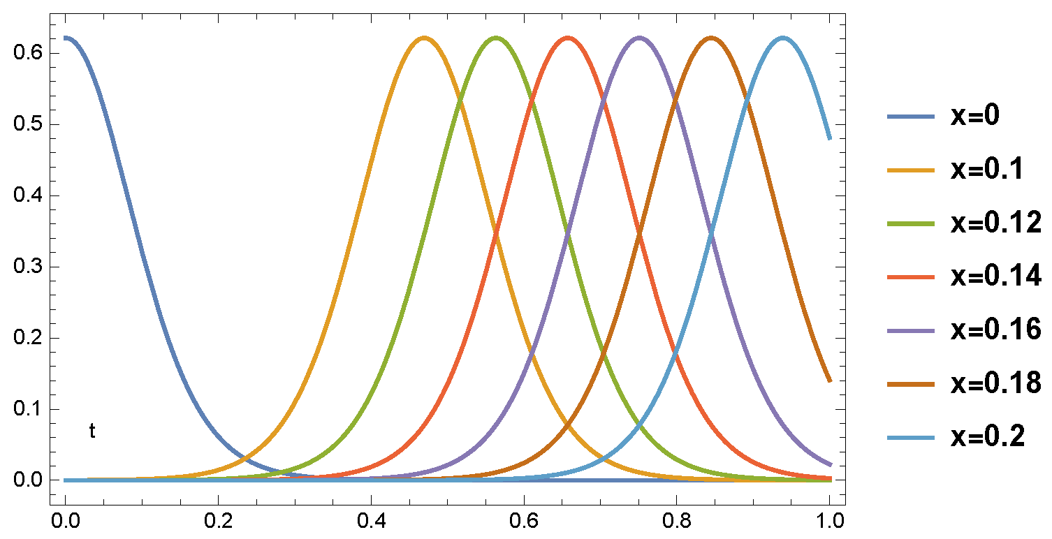
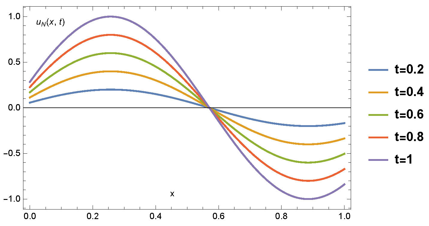
  • Figure 1 presents the numerical solution of Example 1 for various spatial values. From the results in this figure, we can see the moving behavior of the solution wave as x changes.
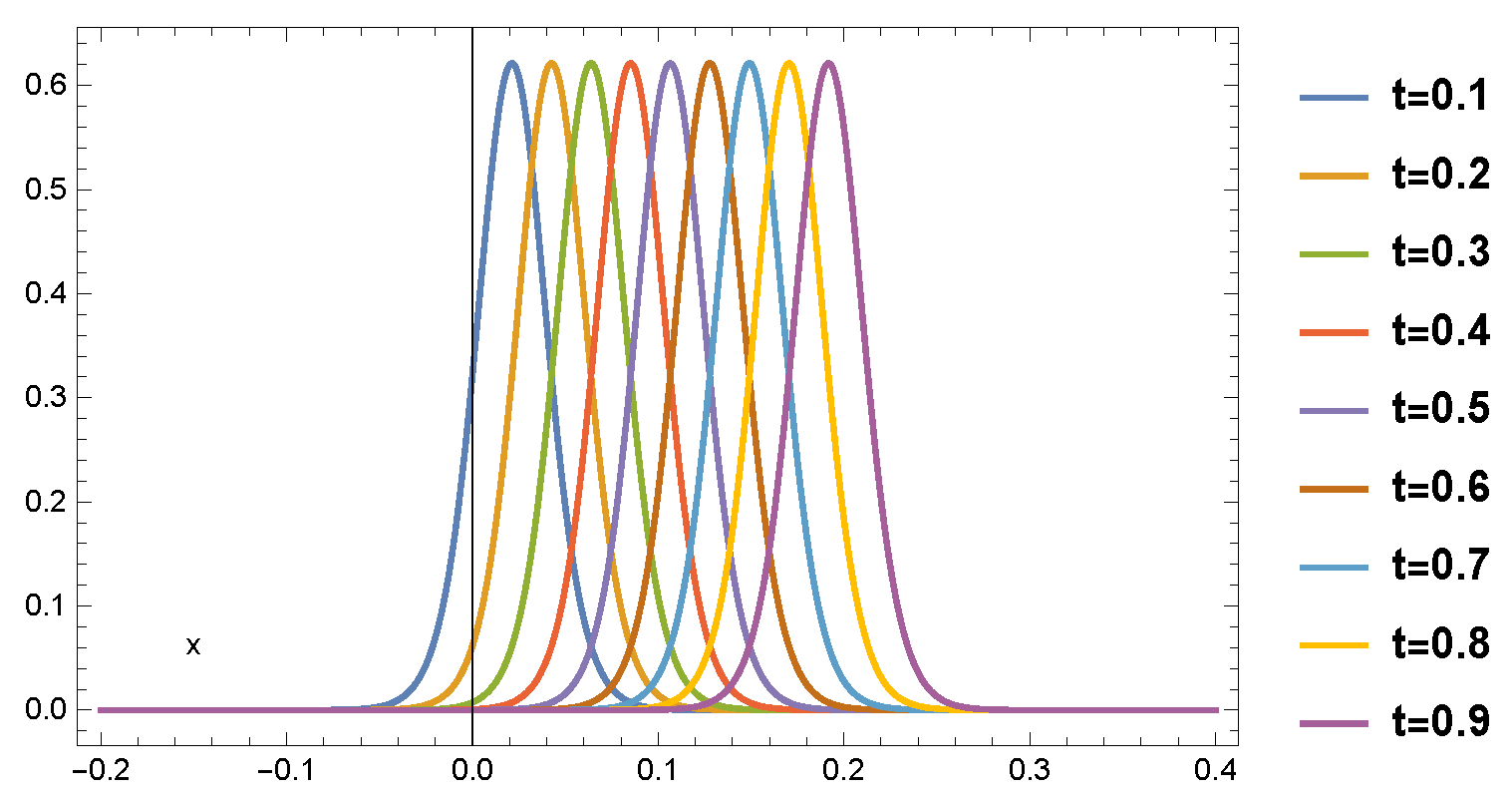
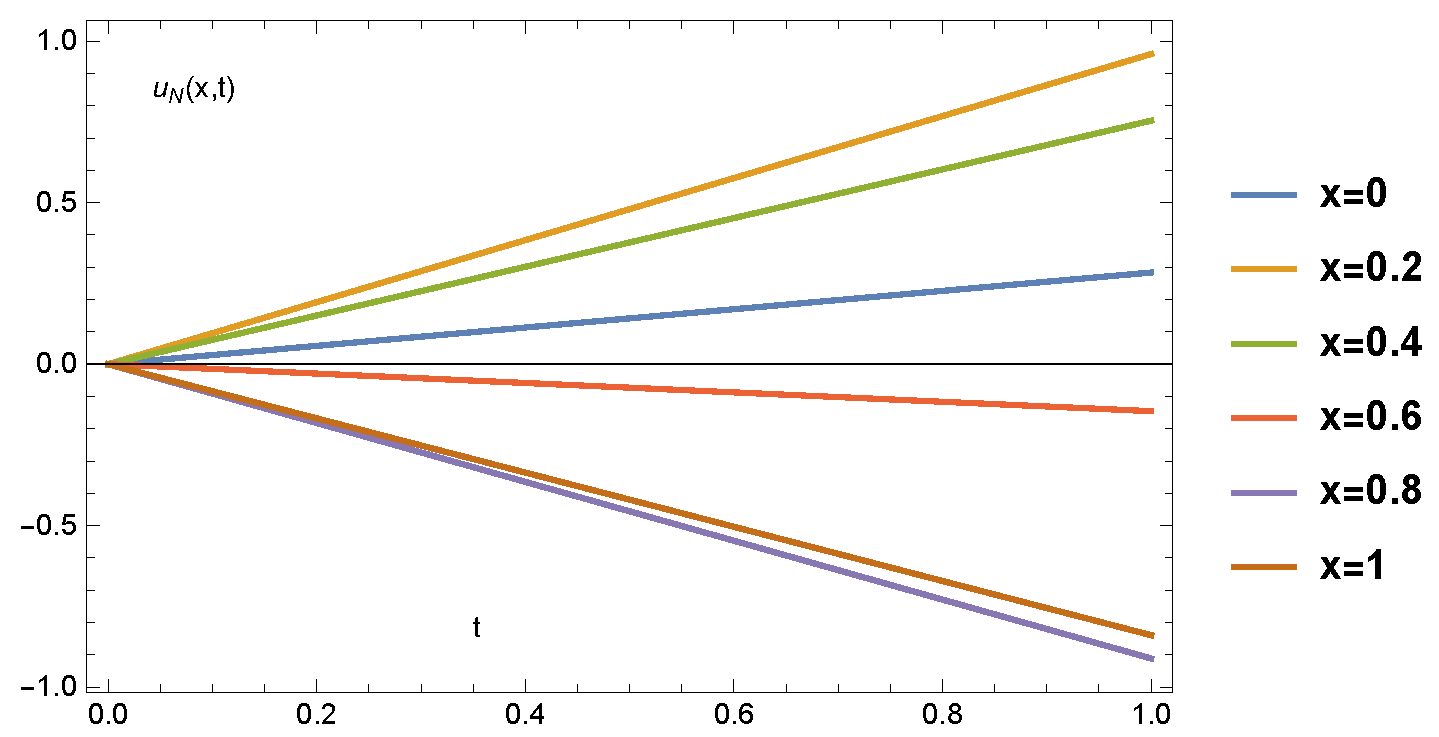
  • Figure 2 presents the numerical solution of Example 1 for various temporal values. From the results in this figure, we can see the infinitesimal change of the solution wave as time goes on for fixed values of x.
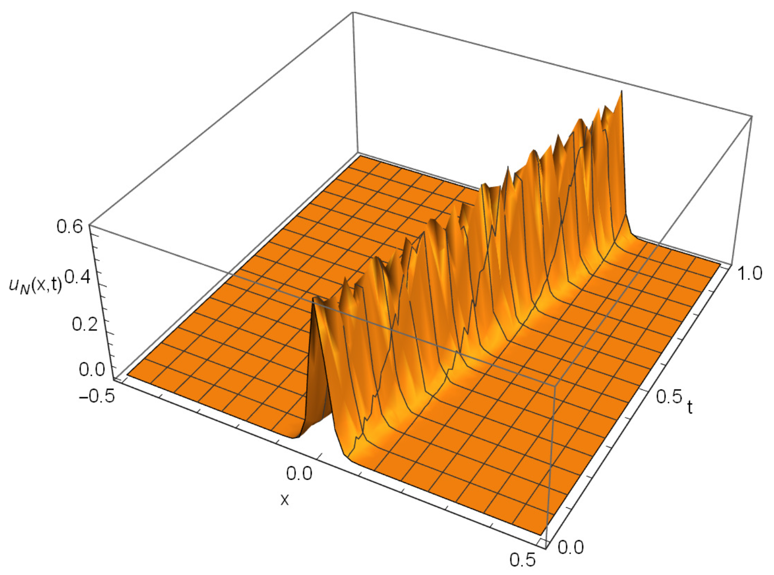
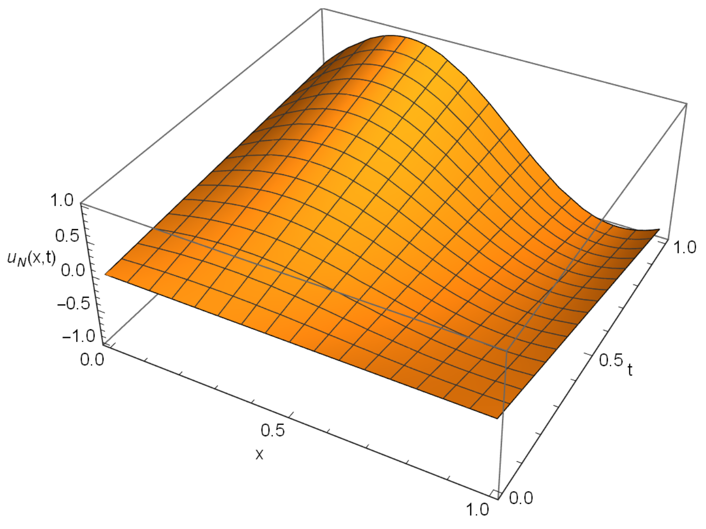
  • Figure 3 presents the numerical solution of Example 1 at any point ( x , t ) Λ . From the results in this figure, we see the whole solution when both temporal and space variable changes, and this wave coincides with the two previous figures.
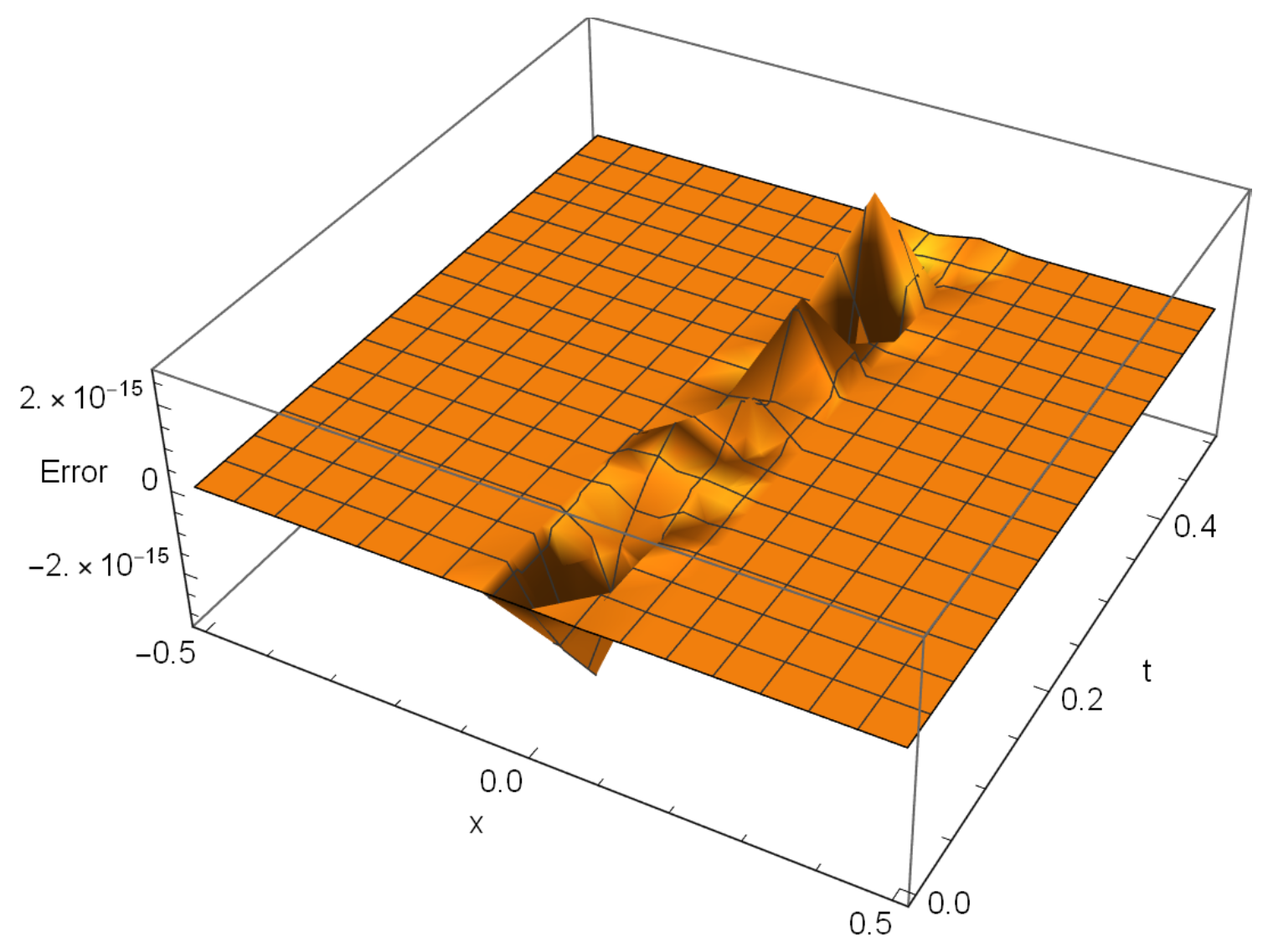
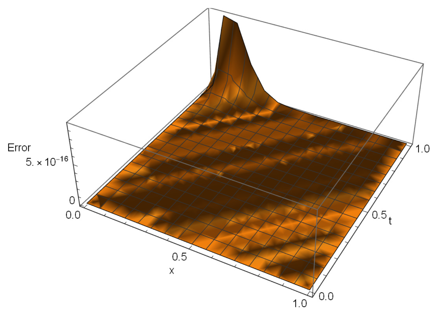
  • Figure 4 presents the absolute error of Example 1 at any point ( x , t ) Λ . From the results in this figure, we ascertain the exponential convergence of the method as the error is of order 10 15 .
In addition, Table 1 displays a comparison between our proposed algorithm with the method developed in [18]. From this comparison, we can definitely conclude that the results obtained by our proposed algorithm were more accurate than those obtained by the method developed in [18].
Example 2
([44]). Consider the following Kawahara equation:
U t + U U x + 3 U x 3 5 U x 5 = 0 , ( x , t ) ( 20 , 30 ) × ( 0 , 30 ) ,
governed by the boundary conditions:
U ( 20 , t ) = U ( 30 , t ) = U x ( 20 , t ) = U x ( 30 , t ) = U x x ( 30 , t ) = 0 ,
and the initial condition:
U ( x , 0 ) = 105 169 sech 4 100 x 13 .
In such a case, a = 20 , b = T = 30 . We applied transformation x ˜ = ( x 5 ) / 25 , t ˜ = t / 30 to obtain the following modified equation:
30 u t + 25 u u x + 15625 u x x x 9765625 u x x x x x = 0 , ( x , t ) Λ = ( 1 , 1 ) × ( 0 , 1 ) ,
subject to the boundary conditions:
u ( ± 1 , t ) = u x ( ± 1 , t ) = u x x ( 1 , t ) = 0 ,
and the initial conditions:
u ( x , 0 ) = 105 169 sech 4 x 5 50 13 ,
with the exact smooth solution
u ( x , t ) = 105 169 sech 4 169 ( x 5 ) 30 t 8450 13 .
We compared our results to those obtained in [44] in Table 2. The results in this table confirm that our method is ultimately better than the cubic spline technique offered in [44]. In Figure 5, we depict the numerical solution for N = 14 over the whole domain.
Example 3
([45]). Consider the following equation:
U t U U x + 5 U x 5 = 0 , ( x , t ) ( 0 , 10 ) × ( 0 , 1 ) ,
governed by the boundary conditions:
U ( 0 , t ) = t , U ( 10 , t ) = t cos 10 , U x ( 0 , t ) = 0 , U x ( 10 , t ) = t sin 10 , U x x ( 1 , t ) = t cos 10 ,
and the initial condition:
U ( x , 0 ) = 0 ,
we apply the transformation x ˜ = 5 ( x + 1 ) , t ˜ = t , to obtain the following modified equation:
u t 0.2 u u x + 0.00032 u x x x x x = 1 2 t 2 sin 10 ( 1 + x ) t sin 5 ( 1 + x ) + cos 5 ( 1 + x ) , ( x , t ) Λ = ( 0 , 1 ) × ( 0 , 1 ) ,
subject to the boundary conditions:
u ( 0 , t ) = t cos 5 , u x ( 0 , t ) = 5 t sin 5 , u ( 1 , t ) = t cos 10 , u x ( 1 , t ) = 5 t sin 10 , u x x ( 1 , t ) = 25 t cos 10 ,
and the initial condition:
u ( x , 0 ) = 0 ,
with the exact smooth solution:
u ( x , t ) = t cos 5 ( 1 + x ) .
We display now some figures whose descriptions are as follows:
  • Figure 6 presents the numerical solution of Example 3 for various spatial values. From the results in this figure, we can track the spatial change of the solution at a fixed instant.
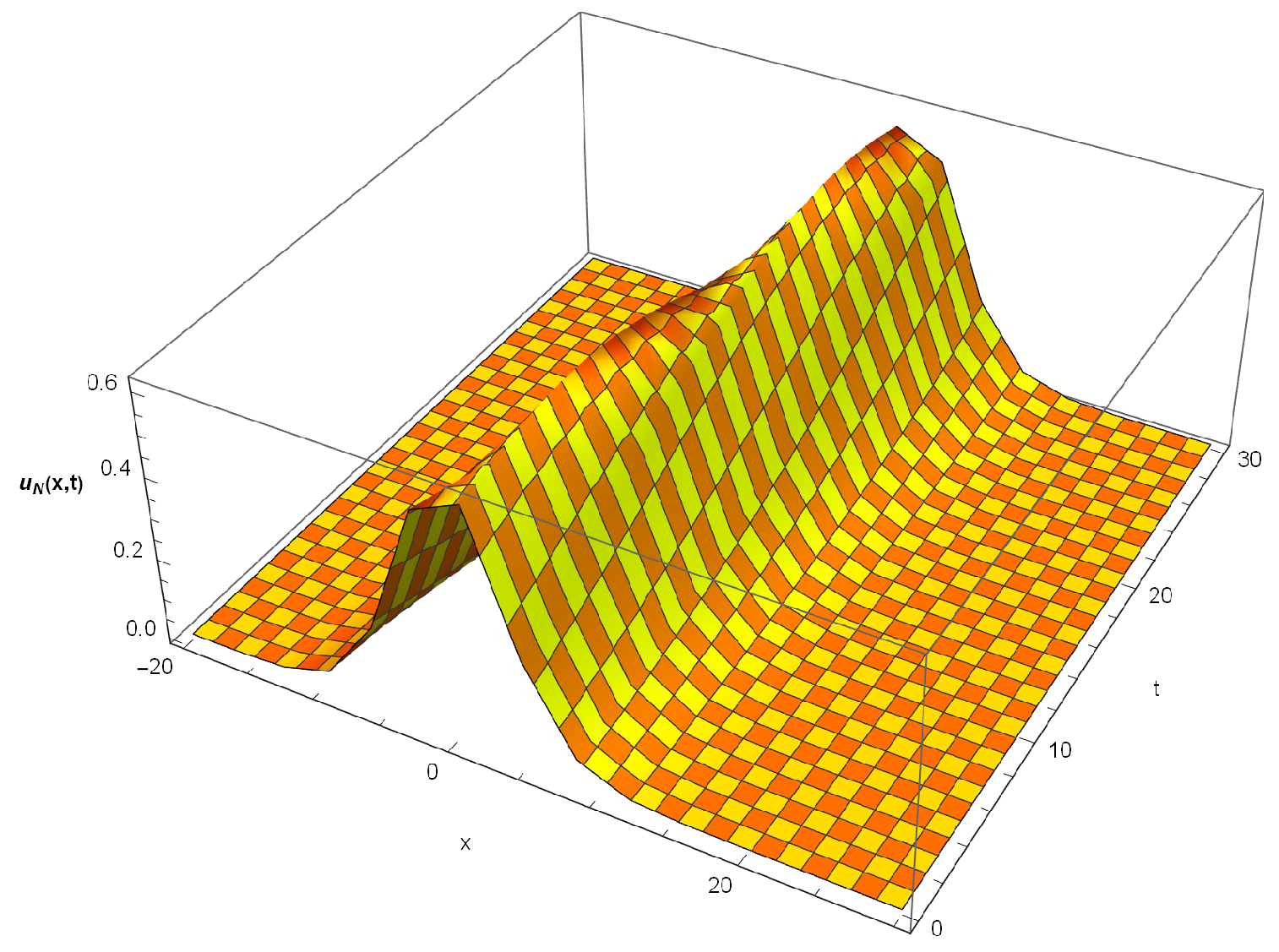
  • Figure 7 presents the numerical solution of Example 3 for various temporal values. From the results in this figure, we can track the temporal change of the solution at a fixed x.
  • Figure 8 presents the numerical solution of Example 3 at any point ( x , t ) Λ . From the results in this figure we can see the whole solution at any point in the x t plane.
  • Figure 9 presents the absolute error of Example 3 at any point ( x , t ) Λ . From the results in this figure, we can clearly verify the accuracy of the method.
Example 4.
We chose to handle the following example with an exact polynomial solution to ensure that the method would achieve the solution if the number of retained modes agrees with the highest degree of the monic polynomial included in the exact solution.
u t + 1 5 u u x + 1 60 u x x x + 1 120 u x x x x x = t 2 x 9 + t x 2 + t + x 5 , ( x , t ) Λ = ( 0 , 1 ) × ( 0 , 1 ) ,
subject to the boundary conditions:
u ( 0 , t ) = u x ( 0 , t ) = 0 , u ( 1 , t ) = t , u x ( 1 , t ) = 5 t , u x x ( 1 , t ) = 20 t ,
and the initial conditions:
u ( x , 0 ) = 0 ,
with the exact smooth solution
u ( x , t ) = x 5 t .
We applied the technique in Section 4.1 for N = 5 . In such a case, the approximate solution is given by
u N ( x , t ) = p = 0 5 q = 0 5 a p , q ϕ p ( x ) ψ q ( t ) .
Furthermore, Equations (60)–(66) yield the following coefficients of the approximate solution expansion:
a 0 , 0 = a 0 , 1 = 93 512 , a 1 , 1 = a 1 , 0 = 225 1024 , a 2 , 1 = a 2 , 0 = 65 256 ,
a 3 , 1 = a 3 , 0 = 57 320 , a 4 , 1 = a 4 , 0 = 5 64 , a 5 , 1 = a 5 , 0 = 1 64 ,
a p , q = 0 , 0 p 5 , 2 q 5 ,
and accordingly, we obtain
u N ( x , t ) = t x 5 ,
which is the exact solution.

6. Conclusions

In this paper, a new spectral solution to the Kawahara-type equations was proposed. The derivation of this solution is based on the application of the Tau method. Two families of the fifth-kind Chebyshev polynomials and their shifted ones were selected as basis functions. Some theoretical results concerning the fifth-kind Chebyshev polynomials and their shifted polynomials were established and utilized to obtain our proposed algorithm. The Tau method served to transform the Kawahara partial differential equation governed by its underlying conditions into a system of nonlinear equations that could be efficiently solved. The numerical examples showed the accuracy and applicability of our proposed algorithm. Our algorithm could be applied to other types of nonlinear differential equations.

Author Contributions

W.M.A.-E. contributed to conceptualization, methodology, software, validation, formal analysis, investigation, Writing—Original draft, Writing—review & editing, and Supervision. S.O.A. contributed to validation and investigation, A.K.A. contributed to validation and funding Acquisition. Y.H.Y. contributed to conceptualization, methodology, software, formal analysis, investigation, Writing—Original draft, Writing—review & editing. All authors have read and agreed to the published version of the manuscript.

Funding

The third author, Amr Kamel Amin ([email protected]), is funded by the Deanship of Scientific Research at Umm Al-Qura University.

Institutional Review Board Statement

Not applicable.

Informed Consent Statement

Not applicable.

Data Availability Statement

Not applicable.

Acknowledgments

The authors would like to thank the Deanship of Scientific Research at Umm Al-Qura University for supporting this work grant code: (22UQU4331287DSR06).

Conflicts of Interest

The authors declare no conflict of interest.

References

  1. Thomas, J.W. Numerical Partial Differential Equations: Finite Difference Methods; Springer Science & Business Media: New York, NY, USA, 2013; Volume 22. [Google Scholar]
  2. Smith, G. Numerical Solution of Partial Differential Equations: Finite Difference Methods; Oxford University Press: Oxford, UK, 1985. [Google Scholar]
  3. Hesthaven, J.S.; Gottlieb, S.; Gottlieb, D. Spectral Methods for Time-Dependent Problems; Cambridge University Press: Cambridge, MA, USA, 2007; Volume 21. [Google Scholar]
  4. Canuto, C.; Hussaini, M.Y.; Quarteroni, A.; Zang, T.A. Spectral Methods in Fluid Dynamics; Springer: Berlin/Heidelberg, Germany, 1988. [Google Scholar]
  5. Abd-Elhameed, W.M. Novel expressions for the derivatives of sixth-kind Chebyshev polynomials: Spectral solution of the non-linear one-dimensional Burgers’ equation. Fractal Fract. 2021, 5, 53. [Google Scholar] [CrossRef]
  6. Singh, H. Jacobi collocation method for the fractional advection-dispersion equation arising in porous media. Numer. Methods Part. Differ. Equ. 2022, 38, 636–653. [Google Scholar] [CrossRef]
  7. Khader, M.; Saad, K.; Hammouch, Z.; Baleanu, D. A spectral collocation method for solving fractional KdV and KdV-Burgers equations with non-singular kernel derivatives. Appl. Numer. Math. 2021, 161, 137–146. [Google Scholar] [CrossRef]
  8. Atta, A.G.; Youssri, Y.H. Advanced shifted first-kind Chebyshev collocation approach for solving the nonlinear time-fractional partial integro-differential equation with a weakly singular kernel. Comput. Appl. Math. 2022, 41, 381. [Google Scholar] [CrossRef]
  9. Canıvar, A.; Sari, M.; Dag, I. A Taylor–Galerkin finite element method for the KdV equation using cubic B-splines. Phys. B Cond. Matter 2010, 405, 3376–3383. [Google Scholar] [CrossRef]
  10. Shen, J. A new dual-Petrov-Galerkin method for third and higher odd-order differential equations: Application to the KDV equation. SIAM J. Numer. Anal. 2003, 41, 1595–1619. [Google Scholar] [CrossRef]
  11. Turgut, A.K.; Karakoç, S.B.G.; Biswas, A. Application of Petrov-Galerkin finite element method to shallow water waves model: Modi ed Korteweg-de Vries equation. Sci. Iran. B 2017, 24, 1148–1159. [Google Scholar]
  12. Noor, M.A.; Noor, K.I.; Waheed, A.; Al-Said, E.A. Some new solitonary solutions of the modified Benjamin–Bona–Mahony equation. Comput. Math. Appl. 2011, 62, 2126–2131. [Google Scholar] [CrossRef] [Green Version]
  13. Yokus, A.; Sulaiman, T.A.; Bulut, H. On the analytical and numerical solutions of the Benjamin–Bona–Mahony equation. Opt. Quantum Electron. 2018, 50, 31. [Google Scholar] [CrossRef]
  14. Wang, K.J.; Wang, G.D. Solitary and periodic wave solutions of the generalized fourth-order Boussinesq equation via He’s variational methods. Math. Methods Appl. Sci. 2021, 44, 5617–5625. [Google Scholar] [CrossRef]
  15. Kawahara, T. Oscillatory solitary waves in dispersive media. J. Phys. Soc. Jpn. 1972, 33, 260–264. [Google Scholar] [CrossRef]
  16. Korkmaz, A.; Dağ, I. Crank-Nicolson–differential quadrature algorithms for the Kawahara equation. Chaos Solitons Fractals 2009, 42, 65–73. [Google Scholar] [CrossRef]
  17. Haq, S.; Uddin, M. RBFs approximation method for Kawahara equation. Eng. Anal. Bound. Elem. 2011, 35, 575–580. [Google Scholar] [CrossRef]
  18. Yuan, J.; Shen, J.; Wu, J. A dual-Petrov-Galerkin method for the Kawahara-type equations. J. Sci. Comput. 2008, 34, 48–63. [Google Scholar] [CrossRef] [Green Version]
  19. Kaya, D. An explicit and numerical solutions of some fifth-order KdV equation by decomposition method. Appl. Math. Comput. 2003, 144, 353–363. [Google Scholar] [CrossRef]
  20. Yusufoğlu, E.; Bekir, A. Symbolic computation and new families of exact travelling solutions for the Kawahara and modified Kawahara equations. Comput. Math. Appl. 2008, 55, 1113–1121. [Google Scholar] [CrossRef] [Green Version]
  21. Jin, L. Application of variational iteration method and homotopy perturbation method to the modified Kawahara equation. Math. Comput. Model. 2009, 49, 573–578. [Google Scholar] [CrossRef]
  22. Yusufoğlu, E.; Bekir, A.; Alp, M. Periodic and solitary wave solutions of Kawahara and modified Kawahara equations by using Sine–Cosine method. Chaos Solitons Fractals 2008, 37, 1193–1197. [Google Scholar] [CrossRef]
  23. Mason, J.C.; Handscomb, D.C. Chebyshev Polynomials; Chapman and Hall: New York, NY, USA; CRC: Boca Raton, FL, USA, 2003. [Google Scholar]
  24. Boyd, J.P. Chebyshev and Fourier Spectral Methods, 2nd ed.; Dover: New York, NY, USA, 2000. [Google Scholar]
  25. Öztürk, Y. Numerical solution of systems of differential equations using operational matrix method with Chebyshev polynomials. J. Taibah Univ. Sci. 2018, 12, 155–162. [Google Scholar] [CrossRef]
  26. Heydari, M.H.; Atangana, A.; Avazzadeh, Z. Chebyshev polynomials for the numerical solution of fractal–fractional model of nonlinear Ginzburg–Landau equation. Eng. Comput. 2021, 37, 1377–1388. [Google Scholar] [CrossRef]
  27. Öztürk, Y.; Gülsu, M. An operational matrix method to solve linear Fredholm–Volterra integro-differential equations with piecewise intervals. Math. Sci. 2021, 15, 189–197. [Google Scholar] [CrossRef]
  28. Öztürk, Y. An efficient numerical algorithm for solving system of Lane–Emden type equations arising in engineering. Nonlinear Eng. 2019, 8, 429–437. [Google Scholar] [CrossRef]
  29. Abdelhakem, M.; Alaa-Eldeen, T.; Baleanu, D.; Alshehri, M.G.; El-Kady, M. Approximating real-life BVPs via Chebyshev polynomials’ first derivative pseudo-Galerkin method. Fractal Frac. 2021, 5, 165. [Google Scholar] [CrossRef]
  30. Abd-Elhameed, W.M.; Ahmed, H.M. Tau and Galerkin operational matrices of derivatives for treating singular and Emden–Fowler third-order-type equations. Int. J. Mod. Phys. 2022, 33, 2250061. [Google Scholar] [CrossRef]
  31. Youssri, Y.H.; Abd-Elhameed, W.M.; Ahmed, H.M. New fractional derivative expression of the shifted third-kind Chebyshev polynomials: Application to a type of nonlinear fractional pantograph differential equations. J. Funct. Spaces 2022, 2022, 3966135. [Google Scholar] [CrossRef]
  32. Duangpan, A.; Boonklurb, R.; Juytai, M. Numerical solutions for systems of fractional and classical integro-differential equations via finite integration method based on shifted Chebyshev polynomials. Fractal Frac. 2021, 5, 103. [Google Scholar] [CrossRef]
  33. Jena, S.K.; Chakraverty, S.; Malikan, M. Application of shifted Chebyshev polynomial-based Rayleigh–Ritz method and Navier’s technique for vibration analysis of a functionally graded porous beam embedded in Kerr foundation. Eng. Comput. 2021, 37, 3569–3589. [Google Scholar] [CrossRef]
  34. Öztürk, Y.; Gülsu, M. An operational matrix method for solving Lane–Emden equations arising in astrophysics. Math. Methods Appl. Sci. 2014, 37, 2227–2235. [Google Scholar] [CrossRef]
  35. Öztürk, Y.; Demir, A.İ. A spectral collocation matrix method for solving linear Fredholm integro-differential–difference equations. Comput. Appl. Math. 2021, 40, 218. [Google Scholar] [CrossRef]
  36. Draux, A.; Sadik, M.; Moalla, B. Markov–Bernstein inequalities for generalized Gegenbauer weight. Appl. Numer. Math. 2011, 61, 1301–1321. [Google Scholar] [CrossRef]
  37. Xu, Y. An integral formula for generalized Gegenbauer polynomials and Jacobi polynomials. Adv. Appl. Math. 2002, 29, 328–343. [Google Scholar] [CrossRef]
  38. Abd-Elhameed, W.M.; Alkhamisi, S.O. New results of the fifth-kind orthogonal Chebyshev polynomials. Symmetry 2021, 13, 2407. [Google Scholar] [CrossRef]
  39. Atta, A.G.; Abd-Elhameed, W.M.; Moatimid, G.M.; Youssri, Y.H. Modal shifted fifth-kind Chebyshev tau integral approach for solving heat conduction equation. Fractal Frac. 2022, 6, 619. [Google Scholar] [CrossRef]
  40. Abd-Elhameed, W.M.; Youssri, Y.H. Fifth-kind orthonormal Chebyshev polynomial solutions for fractional differential equations. Comput. Appl. Math. 2018, 37, 2897–2921. [Google Scholar] [CrossRef]
  41. Masjed-Jamei, M. Some New Classes of Orthogonal Polynomials and Special Functions: A Symmetric Generalization of Sturm-Liouville Problems and Its Consequences. Ph.D. Thesis, Department of Mathematics, University of Kassel, Kassel, Germany, 2006. [Google Scholar]
  42. Abd-Elhameed, W.M.; Youssri, Y.H. New formulas of the high-order derivatives of fifth-kind Chebyshev polynomials: Spectral solution of the convection–diffusion equation. In Numerical Methods for Partial Differential Equations; Wiley: Hoboken, NJ, USA, 2021. [Google Scholar] [CrossRef]
  43. Koepf, W. Hypergeometric Summation, 2nd ed.; Springer Universitext Series; Springer: Berlin/Heidelberg, Germany, 2014. [Google Scholar]
  44. Bagherzadeh, A.S. B-spline collocation method for numerical solution of nonlinear Kawahara and modified Kawahara equations. TWMS J. App. Eng. Math. 2017, 7, 188–199. [Google Scholar]
  45. Goswami, A.; Singh, J.; Kumar, D. Numerical simulation of fifth order KdV equations occurring in magneto-acoustic waves. Ain Shams Eng. J. 2018, 9, 2265–2273. [Google Scholar] [CrossRef]
Figure 1. Approximate solution of Example 1 for various spatial values.
Symmetry 15 00138 g001
Figure 2. Approximate solution of Example 1 for various temporal values.
Symmetry 15 00138 g002
Figure 3. Approximate solution of Example 1 at any point ( x , t ) Λ .
Symmetry 15 00138 g003
Figure 4. Absolute error of Example 1 at any point ( x , t ) Λ .
Symmetry 15 00138 g004
Figure 5. Approximate solution of Example 3 at any point ( x , t ) Λ , when N = 14 .
Symmetry 15 00138 g005
Figure 6. Approximate solution of Example 3 for various spatial values.
Symmetry 15 00138 g006
Figure 7. Approximate solution of Example 3 for various temporal values.
Symmetry 15 00138 g007
Figure 8. Approximate solution of Example 3 at any point ( x , t ) Λ .
Symmetry 15 00138 g008
Figure 9. Absolute error of Example 3 at any point ( x , t ) Λ .
Symmetry 15 00138 g009
Table 1. Comparison between L 2 errors of Example 1.
tMethod in [18]Present Method
0.5 3.44 × 10 7 2.78 × 10 15
1 5.93 × 10 7 4.59 × 10 15
Table 2. Comparison between L 2 -errors of Example 2.
tMethod in [44]Present Method ( N = 14 )
5 3.289 × 10 5 6.361 × 10 16
15 3.294 × 10 5 4.273 × 10 16
25 3.320 × 10 5 5.84 × 10 15
Disclaimer/Publisher’s Note: The statements, opinions and data contained in all publications are solely those of the individual author(s) and contributor(s) and not of MDPI and/or the editor(s). MDPI and/or the editor(s) disclaim responsibility for any injury to people or property resulting from any ideas, methods, instructions or products referred to in the content.

