Conductive Heat Transfer in Materials under Intense Heat Flows

Abstract

The paper presents the solution of the spatial transient problem of the impact of a moving heat flux source induced by the laser radiation on the surface of a half-space using the superposition principle and the method of transient functions. The hyperbolic equation of transient thermal conductivity accounting for the relaxation time is used to model the laser heating process. It is assumed that the heat flux is distributed symmetrically with respect to the center of the heating spot. The combined numerical and analytical algorithm has been developed and implemented, which allows one to determine the temperature distribution both on the surface and on the depth of the half-space. In this case, the principle of superposition is used with the use of a special symmetric Gaussian distribution to describe the model of a source of high-intensity heat flux. The use of such a symmetric distribution made it possible to calculate the integrals over the spatial variables analytically. The results of the work could be used to estimate the contribution of the conductive component in the overall heat transfer of materials exposed to intense heat flows (laser surface treatment, laser additive technologies, streamlining and heating of materials by high-enthalpy gases, etc.).

1. Introduction

Due to the rapid development of modern technologies and the creation of new materials, a fairly wide range of problems in physics and continuum mechanics has now formed, to which classical methods of solving problems of heat transfer in solids in their pure form are inapplicable. Microelectronics, micro and nanotechnology, fuel cell production, hybrid engine design, various fields of modern medicine, mechanics of composite materials, laser sintering technology, construction, shipbuilding, aviation, and many other branches of science and industry require the development of modernized theories of heat transfer for an adequate description of heat transfer processes taking place in bodies and structural elements with complex non-classical properties. In addition to force impacts, the products of modern technology and engineering structures are exposed to a complex of physical impacts of various kinds: high temperature, radiation, climatic factors in many cases performing heat-insulating functions. Intensive development of methods and technologies allowing to generate and use flows of thermal radiation of high power and short duration, possibility of application of concentrated energy flows in various fields of modern technologies from medicine and biotechnology to methods of creation, and processing of modern materials and destruction of rocks, leads to the necessity of creating mathematical models of media and elements of structures having non-classical complicated properties, as well as studying a variety of physical and chemical properties. Nowadays, the problems of constructing mathematical models of high-speed transient processes in bodies and structural elements with complex properties remain topical.

The classical theory of coupled thermoelasticity [1] has been proposed by Bio. This theory assumes a theoretically unreasonable unbounded rate of heat propagation. It should be noted that although this consequence of the theory is not realized in practice, classical thermoelasticity quite accurately describes processes, the running time of which is sufficiently long. For example, in quasi-static and static problems for bodies of sufficiently large dimensions, the solution can be obtained with a sufficient degree of accuracy using classical theory.

To eliminate the contradiction related to the infinite velocity of the body, nonclassical theories of thermoelasticity, also called generalized models of thermoelasticity, have been formulated. The main ones are the Lord–Schulman [2], Green–Lindsey [3], Green–Naghdy [4,5], and Moore–Gibson–Thompson [6,7] theories. These theories play an important role in almost all current research in generalized thermoelasticity.

A generalized model of the Lord–Schulman thermoelastic medium, based on the Cattaneau–Vernotte thermal conductivity law, which takes into account the relaxation time of the heat flux, was proposed in [2].

Later, Green and Lindsey proposed a theory with two relaxation parameters, which allows one to take into account the rate of temperature change. The Green–Nagdy thermoelasticity is also widely used (there are three alternative theories, which Green and Nagdy called Type I, Type II and Type III theories). The Green–Nagdi theory is based on the Fourier law, in the right side of which there is a temperature displacement gradient proportional to the free range of the particles. This term makes a tangible contribution to the temperature on scales comparable to the free path length of the molecules.

In recent decades, the Moore–Gibson–Thompson model has been widely used in studies of thermal conductivity and thermoelasticity in new materials. For the first time, the Moore–Gibson–Thompson equation was used in [8] as applied to the compressible fluid model. The Moore–Gibson–Thompson equation is a generalization of the Green–Nagdi theory. This generalization consists in introducing heat flow relaxation time into the Green–Nagdi equation. Thus, the Moore–Gibson–Thompson model can be seen as a union of the Lord–Schulman and Green–Nagdy type III models. Based on this model, Quintanilla in [6,7] constructed a variant of the generalized theory of thermoelasticity. It should be noted that variants of such theories, their understanding and explanation in recent years have aroused great interest.

Classical theories of heat conduction as applied to solving various complex problems of mechanics were used in [9,10,11,12].

In articles [13,14,15,16], approaches to the creation of coupled generalized models of thermoelasticity, thermoviscoelasticity, and magnetothermoelasticity are developed.

Ehringen’s ideas and the type III Green–Nagdy hyperbolic thermoelasticity model were used in [17,18,19,20,21]. The propagation of time-harmonic thermoelastic plane waves in an infinite nonlocal elastic Ehringen–Green–Nagdy continuum was studied in [22].

Nonlocal gradient models of thermoelasticity are built in [23,24,25,26,27].

The Ehringen concept and the Moore–Gibson–Thompson theory of thermoelasticity were used in [28,29].

Methods for creating and using various models of the generalized theory of thermal conductivity can be found in publications [30,31,32,33,34]. A numerical approach to the study of such problems is demonstrated in the article [35].

In this paper, based on the generalized equation of hyperbolic heat conduction, accounting for the relaxation time, a mathematical model of the process of heating the surface of a half-space by a high-intensity source of heat flux is constructed. Along with the available results concerning the Green’s functions for the classical heat equation, an analytical expression for the spatial non-stationary Green’s function in the case of a generalized theory equation with relaxation time taken into account was not found before the publication of this work. This is due to the impossibility of analytical construction of the original of the Green’s function according to Fourier and Laplace using traditional methods of inverting integral transformations. This article proposes an alternative analytical method for inverting the integral Fourier and Laplace transforms, based on the expansion of the desired function in a Fourier series on a variable interval. The use of this approach made it possible to construct the original of the Green’s function by analytical methods. From a practical point of view, this result opens up possibilities for solving a wide range of new problems in the generalized theory of heat conduction. These include problems of surface heating of a substance by high-intensity energy flows, inverse non-stationary problems of generalized thermal conductivity, and also, in the future, problems of a generalized elasticity term. It should be noted that the proposed method of inverting coupled integral transformations can be applied not only to the case of the generalized thermal conductivity model presented in the article, but also in other cases where traditional analytical inversion is impossible or leads to great difficulties. For example, for more complex models of thermal conductivity or thermoelasticity, the proposed method can also be used.

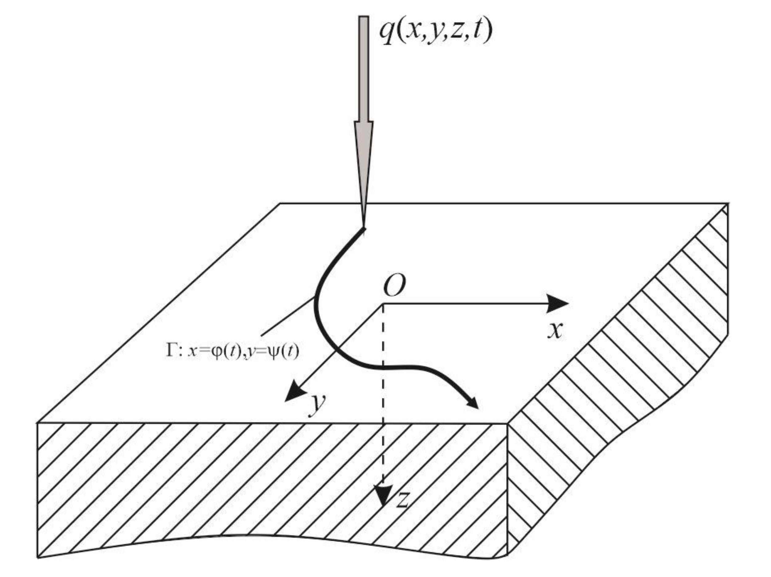
2. Formulation of the Problem

Assume that at the initial time moment $t=0$ at the origin of the rectangular Cartesian coordinate system $Oxyz$ normally attached to the surface of the half-space $z\ge 0$ the heat source $q$ begins to act and moves across the surface of the half-space $z=0$ according to an arbitrary law in time (Figure 1). The flux density $q$ is distributed over the heating spot of radius $R$ in general, it can depend both on the radius $r\in \left[0,R\right]$ and time:

$$q=q\left(x,y,t\right)=q\left(r,t\right)H\left(r-R\right), r=\sqrt{x^2+y^2},$$

(1)

where $H\left(\cdot \right)$ is the Heaviside distribution. It is assumed that the heat flux is distributed symmetrically with respect to the center of the heating spot.

The coordinates of the heating spot center at the moments of time $t>0$ are determined by the parametric dependences:

$$x=\mathsf{\phi }\left(t\right), y=\mathsf{\psi }\left(t\right).$$

(2)

The hyperbolic heat conduction equation allows us to describe the wave nature of heat propagation. It is based on the generalized heat conduction law proposed independently by Cattaneo [36], Vernotte [37], and Lykov [38]:

$$q+{\mathsf{\tau }}_r\frac{\partial q}{\partial t}=-\lambda \mathrm{grad}\mathsf{\vartheta },$$

(3)

where $q$ is the heat flux vector, $\mathsf{\vartheta }$ is the temperature increment, ${\mathsf{\tau }}_r$ is the relaxation time, $\lambda$ is the heat transfer coefficient.

Taking into account the balance equation of internal energy:

$$\mathsf{\rho }\frac{\partial U}{\partial t}=-\mathrm{div}q+q_V,$$

(4)

where $U$ is the internal energy, $\mathsf{\rho }$ is the mass density, $q_v$ is the volumetric density of heat sources, and the dependence of the internal energy on temperature could be represented as follows:

$$U=c_v\mathsf{\vartheta },$$

(5)

where $c_v$ is the specific heat capacity at constant volume. As a result, we obtain:

$$\mathsf{\rho }{c}_v\frac{\partial \mathsf{\vartheta }}{\partial t}=-\mathrm{div}q+q_V.$$

(6)

Applying the divergence operator to (3), we get the equation:

$$\mathrm{div}q+{\mathsf{\tau }}_r\mathrm{div}\frac{\partial q}{\partial t}=-\lambda \Delta \mathsf{\vartheta }.$$

(7)

From Equations (6) and (7) we get:

$$\mathsf{\rho }{c}_v\frac{\partial \mathsf{\vartheta }}{\partial t}=\lambda \Delta \mathsf{\vartheta }+{\mathsf{\tau }}_r\mathrm{div}\frac{\partial q}{\partial t}+q_V.$$

(8)

By differentiating Equation (6) in time, expressing from the resulting equation $\mathrm{div}\frac{\partial q}{\partial t}$ and substituting then the result into Equation (8), we arrive at the hyperbolic Maxwell–Cattaneo heat conduction equation:

$${\mathsf{\tau }}_r\frac{{\partial }^2\mathsf{\vartheta }}{\partial t^2}+\frac{\partial \mathsf{\vartheta }}{\partial t}=a\Delta \mathsf{\vartheta }+\frac{q_V+{\mathsf{\tau }}_r{\dot{q}}_V}{\mathsf{\rho }{c}_v}, \Delta =\frac{{\partial }^2}{\partial x^2}+\frac{{\partial }^2}{\partial y^2}+\frac{{\partial }^2}{\partial z^2}.$$

(9)

where $a=\lambda /c_v\mathsf{\rho }$ is the diffusivity coefficient.

Let us introduce dimensionless values (dimensionless parameters are marked as primed letters):

$$\mathsf{\tau }=\frac{t}{{\mathsf{\tau }}_r}, x^{\prime }=\frac{x}{L}, y^{\prime }=\frac{y}{L}, z^{\prime }=\frac{z}{L}, L=\sqrt{a{\mathsf{\tau }}_r}, {\mathsf{\vartheta }}^{\prime }=\frac{\mathsf{\vartheta }}{T_0}, {q^{\prime }}_v=\frac{q_v{\mathsf{\tau }}_r}{\mathsf{\rho }{c}_v{T}_0},$$

(10)

where $L$ is the characteristic linear dimension, $T_0$ is the characteristic temperature value. In the following text of the article, all variables and parameters have a dimensionless form, while primes for dimensionless quantities are omitted.

Taking into account Equation (10), the Equation (9) will take the dimensionless form:

$$\ddot{\mathsf{\vartheta }}+\dot{\mathsf{\vartheta }}=\Delta \mathsf{\vartheta }+Q_v,$$

(11)

where $Q_v=q_v+{\mathsf{\tau }}_r{\dot{q}}_v$. Hereinafter, the dot denotes the derivative over the dimensionless time τ.

Let us assume that a heat flux is given at the boundary $z=0$

$${\left.-\frac{\partial \mathsf{\vartheta }}{\partial z}\right|}_{z=0}=q\left(x,y,\mathsf{\tau }\right).$$

(12)

Using the substitution $\mathsf{\vartheta }=\mathsf{\theta }{e}^{-\mathsf{\tau }/2}$:

$$\dot{\mathsf{\vartheta }}=e^{-\mathsf{\tau }/2}\left(\dot{\mathsf{\theta }}-\frac{\mathsf{\theta }}{2}\right), \ddot{\mathsf{\vartheta }}=e^{-\mathsf{\tau }/2}\left(\ddot{\mathsf{\theta }}-\dot{\mathsf{\theta }}+\frac{\mathsf{\theta }}{4}\right), \ddot{\mathsf{\vartheta }}+\dot{\mathsf{\vartheta }}=e^{-\mathsf{\tau }/2}\left(\ddot{\mathsf{\theta }}-\dot{\mathsf{\theta }}+\frac{\mathsf{\theta }}{4}+\dot{\mathsf{\theta }}-\frac{\mathsf{\theta }}{2}\right)=e^{-\mathsf{\tau }/2}\left(\ddot{\mathsf{\theta }}-\frac{\mathsf{\theta }}{4}\right)$$

The Equation (11) is reduced to the Klein–Gordon equation with respect to $\mathsf{\theta }$:

$$\ddot{\mathsf{\theta }}-\mathsf{\theta }/4=\Delta \mathsf{\theta }+Q_v{e}^{\mathsf{\tau }/2}.$$

(13)

Initial conditions for definiteness are assumed to be homogeneous

$${\left.\mathsf{\theta }\right|}_{\mathsf{\tau }=0}={\left.\dot{\mathsf{\theta }}\right|}_{\mathsf{\tau }=0}=0.$$

(14)

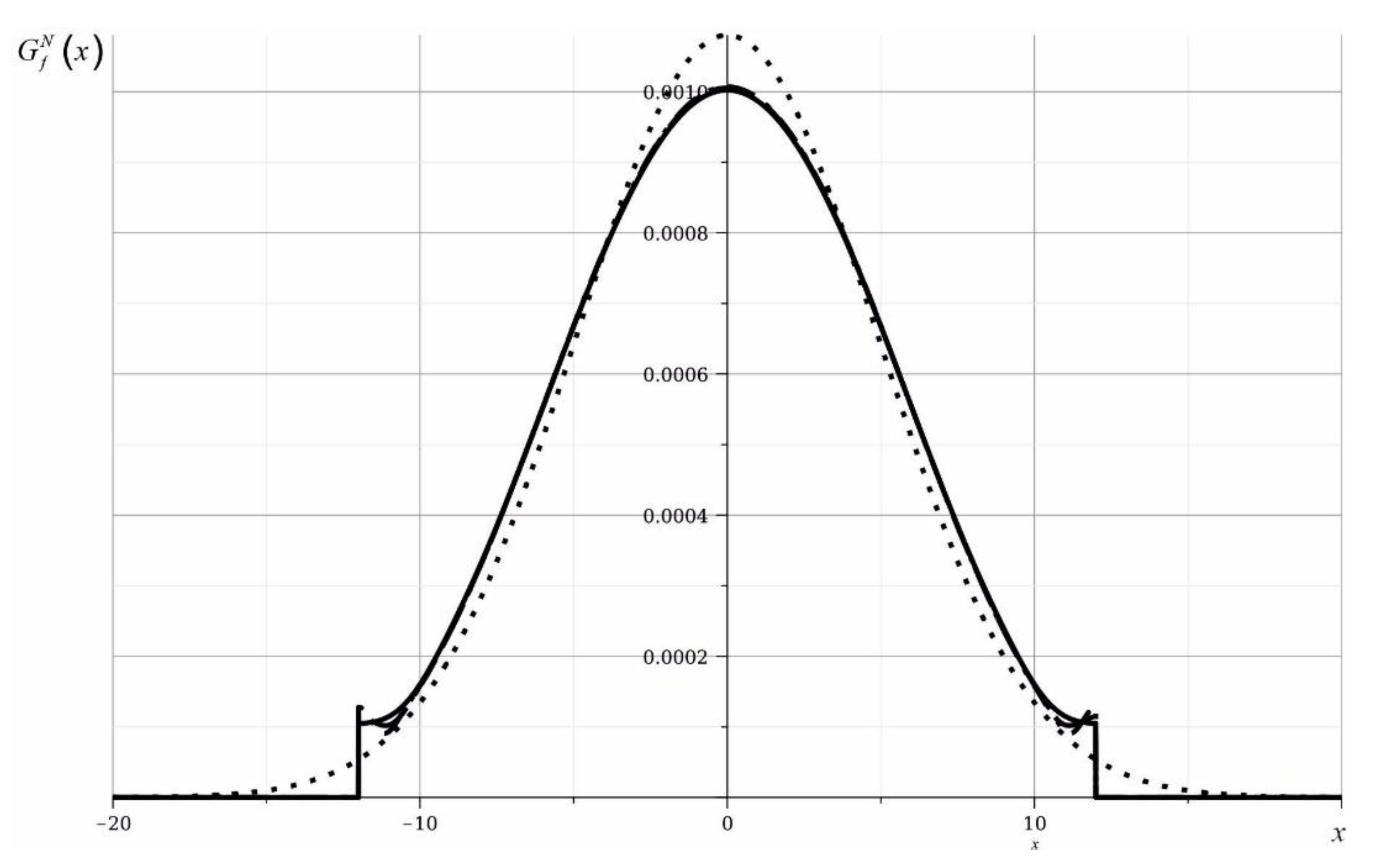
3. The Surface Spatial Transient Function

Green’s functions (transient functions) play an important role in solving practical problems. In fact, they represent the response of the considered body or medium to the impact of a single concentrated source of perturbations. These functions can be superficial or volumetric. In the case of heat conduction problems, the surface transient function is used to construct solutions to problems on the action of arbitrary surface heat flux sources. Thus, the surface transient function contains all the information about the reaction of a body to arbitrary heating of its surface by a heat flux and allows one to obtain solutions to any direct problems of surface heating in quadratures.

Assume that the surface of the half-space is affected by the heat flux vector $q$ directed along the normal to the surface of the half-space (Figure 1).

Let us pose the problem of the impact on the surface of a half-space $z=0$ of a heat flux $q$ of a special form:

$$q=\mathsf{\delta }\left(x,y\right)\mathsf{\delta }\left(\mathsf{\tau }\right),$$

(15)

where $\mathsf{\delta }\left(x,y\right)$, $\mathsf{\delta }\left(\mathsf{\tau }\right)$ are the Dirac delta distributions. The heat flux specified in this way is a mathematical model of a surface heat source concentrated in coordinates and time, which acts on the boundary of the half-space at the origin of the coordinate system. There are no other heat sources in the half-space: $Q_v=0$. Then the corresponding initial-boundary value problem follows from Equations (12)–(14) and has the form

$${\ddot{F}}_f-{\mathsf{\beta }}^2{F}_f=\Delta F_f, {\left.F_f\right|}_{\mathsf{\tau }=0}={\left.{\dot{F}}_f\right|}_{\mathsf{\tau }=0}=0, {\left.-\frac{\partial F_f}{\partial z}\right|}_{z=0}=\mathsf{\delta }\left(x,y\right)\mathsf{\delta }\left(\mathsf{\tau }\right), {\left.F_f\right|}_{z\to \infty }=O\left(1\right)$$

(16)

$$G_f\left(x,y,z,\mathsf{\tau }\right)=e^{-\mathsf{\beta }\mathsf{\tau }}{F}_f.$$

(17)

Here a function $F_f$ is introduced corresponding to the previously introduced auxiliary function $\mathsf{\theta }$ in Equation (13), which must satisfy the condition on the action of a concentrated heat source of a special form Equation (15) and the attenuation condition at infinity. In this case, the temperature field $G_f\left(x,y,z,\mathsf{\tau }\right)$ is related to the function $F_f$ by expression Equation (17). The function $G_f\left(x,y,z,\mathsf{\tau }\right)$ is a non-stationary surface spatial transient function. We also note that the boundary condition Equation (12) remains valid for the auxiliary function $F_f$, when the Laplace transform in time is used in the future.

Note that the transient function $G_f\left(x,y,z,\mathsf{\tau }\right)$ has a cylindrical symmetry. This property is provided by the central symmetry of the delta function $\mathsf{\delta }\left(x,y\right)$.

To solve problem Equation (16), we use the Fourier and Laplace integral transforms ($p_i,s$, $i=1,2$ are the parameters of these transforms):

$$F_f^{FL}\left(p_1,p_2,z,s\right)={\displaystyle \underset{0}{\overset{\infty }{\int }}{e}^{-s\mathsf{\tau }}d\mathsf{\tau }{\displaystyle \underset{-\infty }{\overset{\infty }{\int }}{e}^{i{p}_{1}x}dx{\displaystyle \underset{-\infty }{\overset{\infty }{\int }}{F}_f\left(x,y,z,\mathsf{\tau }\right)e^{i{p}_{2}y}dy}}}, {\left[\mathsf{\delta }\left(x,y\right)\mathsf{\delta }\left(\mathsf{\tau }\right)\right]}^{FL}=1.$$

(18)

Then, the problem Equation (16) takes the form Equation (19) in the image space:

$$\frac{{\partial }^2{F}_f^{FL}}{\partial z^2}-(s^2+p^2-1/4)F_f^{FL}=0,-{\left.\frac{\partial F_f^{FL}}{\partial z}\right|}_{z=0}=1, {\left.F_f^{FL}\right|}_{z\to \infty }=O\left(1\right), p^2=p_1^2+p_2^2.$$

(19)

Taking into account the boundedness at infinity, the solution to Equation (19) is the following function

$$F_f^{FL}=C{e}^{-z\sqrt{s^2+p^2-1/4}}.$$

(20)

We find the constant from the boundary condition ${\left.-\frac{\partial F_f^{FL}}{\partial z}\right|}_{z=0}=1$:

$$C\sqrt{s^2+p^2-1/4}=1, C={\left(s^2+p^2-1/4\right)}^{-1/2}.$$

(21)

Then the image of the function $F_f$ will take the form

$$F_f^{FL}=\frac{e^{-z\sqrt{s^2+p^2-1/4}}}{\sqrt{s^2+p^2-1/4}}.$$

(22)

Let us perform the inverse Laplace transformation [39]:

$$F_f^F\left(p_1,p_2,z,\mathsf{\tau }\right)=H\left(\mathsf{\tau }-z\right)J_0\left[\sqrt{\left({\mathsf{\tau }}^2-z^2\right)\left(p^2-1/4\right)}\right].$$

(23)

The formula for the analytical inversion of the two-dimensional integral Fourier transform for Equation (23) can be constructed using the connection of the integral Fourier transform with the Fourier series on a variable interval [40,41,42,43,44,45,46]:

$$\begin{gathered} F_f\left(x,y,z,\mathsf{\tau }\right)=\frac{1}{4{\pi }^2}{\displaystyle \underset{-\infty }{\overset{\infty }{\int }}{\displaystyle \underset{-\infty }{\overset{\infty }{\int }}{F}_f^F\left(p_1,p_2,z,\mathsf{\tau }\right)e^{-i\left(p_1{x}_1+p_2{x}_2\right)}}d{p}_1}d{p}_2= \\ \frac{1}{4{\mathsf{\tau }}^2}\cdot {\displaystyle \sum _{n=-\infty }^{\infty }{\displaystyle \sum _{m=-\infty }^{\infty }{F}_f^F\left(p_n,p_m,z,\mathsf{\tau }\right)}}{e}^{-i\left(p_{n}x+p_{m}y\right)}, p_n=\frac{\pi n}{\mathsf{\tau }}, p_m=\frac{\pi m}{\mathsf{\tau }}. \end{gathered}$$

(24)

Thus, for the original of the influence function, we obtain the formula

$$G_f\left(x,y,z,\mathsf{\tau }\right)=\frac{e^{-\mathsf{\tau }/2}}{4{\mathsf{\tau }}^2}\cdot {\displaystyle \sum _{n=-\infty }^{\infty }{\displaystyle \sum _{m=-\infty }^{\infty }{F}_f^F\left(p_n,p_m,z,\mathsf{\tau }\right)}}{e}^{-i\left(p_{n}x+p_{m}y\right)}.$$

(25)

For practical purposes, the limits of the sums in Equation (25) should be taken equal to some sufficiently large integer $N>0$ and the approximate formula should be used

$$G_f\left(x,y,z,\mathsf{\tau }\right)\approx G_f^N\left(x,y,z,\mathsf{\tau }\right)=\frac{e^{-\mathsf{\tau }/2}}{4{\mathsf{\tau }}^2}\cdot {\displaystyle \sum _{n=-N}^N{\displaystyle \sum _{m=-N}^N{F}_f^F\left(p_n,p_m,z,\mathsf{\tau }\right)}}{e}^{-i\left(p_{n}x+p_{m}y\right)}.$$

(26)

In Figure 2, the dependences of the influence function on the coordinate at $y=z=0$, $\mathsf{\tau }=12$ taking into account a different number of terms in series Equation (26) are showed. The solid curve corresponds to $N=10$, the dashed curve corresponds to $N=15$, and the dash-dotted curve corresponds to $N=20$. The dotted line on the graph corresponds to the known fundamental solution $G_c$ of the classical heat equation $G_c\left(x,y,z,\mathsf{\tau }\right)=\frac{e^{-r^2/4\mathsf{\tau }}}{4{\left(\pi \mathsf{\tau }\right)}^{3/2}}, r^2=x^2+y^2+z^2$. The breaks in the graphs correspond to the position of the heat wave front. Its presence is explained by the finite value of the velocity of propagation of thermal waves in the case of the generalized theory of heat conduction. It can be seen from the figure that there is a practical convergence of the results. In further calculations, it is assumed everywhere $N=20$.

Comparison with the results of the classical theory as a function of time is shown in Figure 3. Here, the solid curve corresponds to the found generalized influence function $G_f$, and the dashed curve corresponds to the known fundamental solution of the classical heat equation $G_c$. The figure shows the dependences on time at the point with coordinates $x=3$, $y=z=0$. There is a difference in the results at the initial time points. Then, starting from the moment of time $\mathsf{\tau }=4$, the results of the generalized theory practically coincide with the results of the classical theory. Therefore, it is advisable to use the theory of generalized thermal conductivity in cases of short-term high-intensity thermal effects, for example, during pulsed laser heating.

4. Symmetric Model of a Laser Pulse Source

Assume that the distribution of the heat flux q over the surface of the half-space is independent of time and obeys the symmetric Gaussian distribution law:

$$q=q\left(\mathsf{\xi },\mathsf{\zeta }\right)=\frac{Q{e}^{-\frac{{\mathsf{\xi }}^2+{\mathsf{\zeta }}^2}{2{\mathsf{\sigma }}^2}}}{2\pi {\mathsf{\sigma }}^2},$$

(27)

where $Q$ is the laser source power, σ is the standard deviation.

By the property of the Gaussian function ${\displaystyle \underset{-\infty }{\overset{\infty }{\int }}{\displaystyle \underset{-\infty }{\overset{\infty }{\int }}q\left(\mathsf{\xi },\mathsf{\zeta }\right)d\mathsf{\xi }d\mathsf{\zeta }}}=Q$.

By selecting one or another value of the standard deviation, you can adjust the radius of the heating spot carrier [44,45].

5. Integral Representation of the Solution

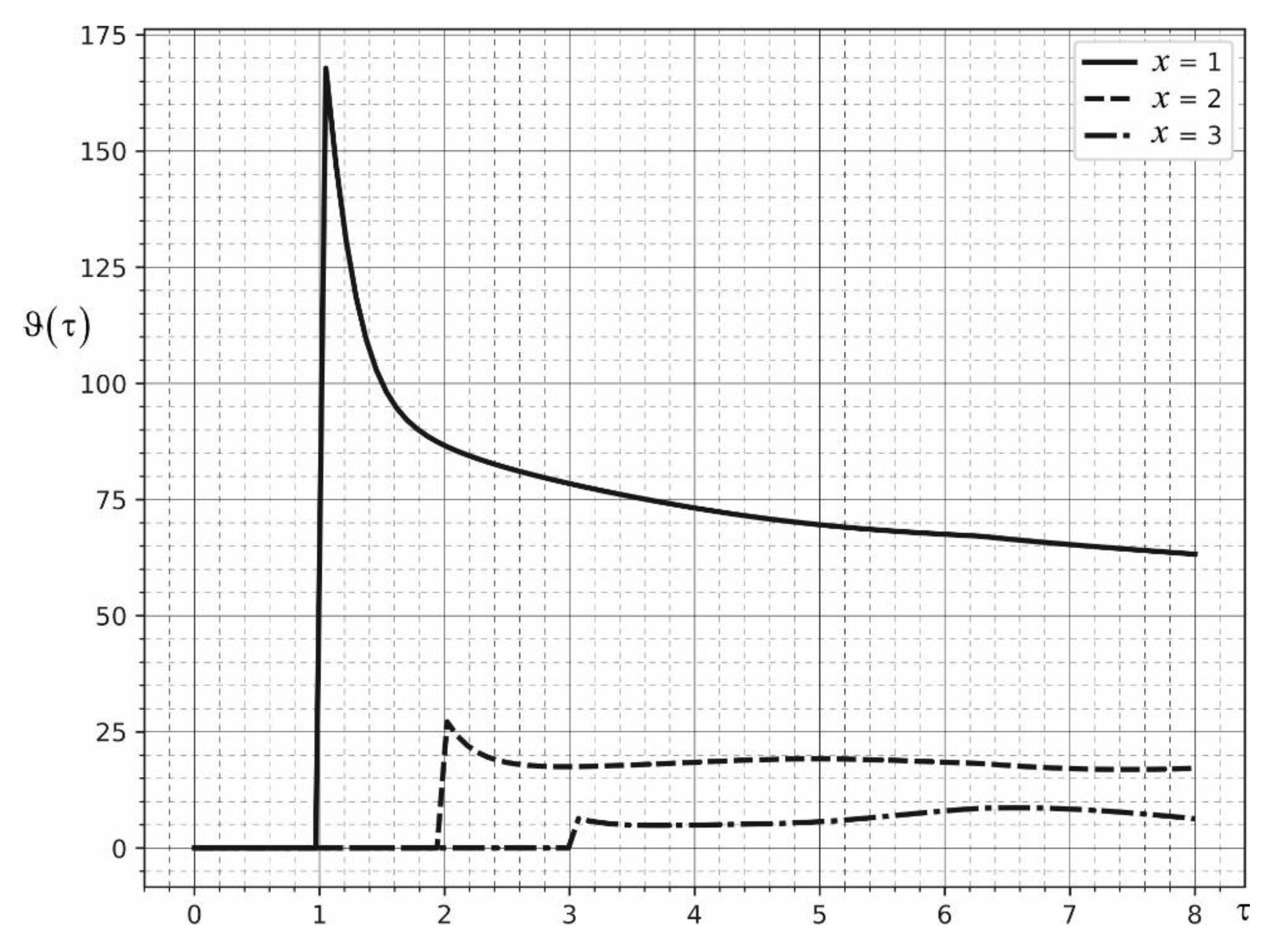
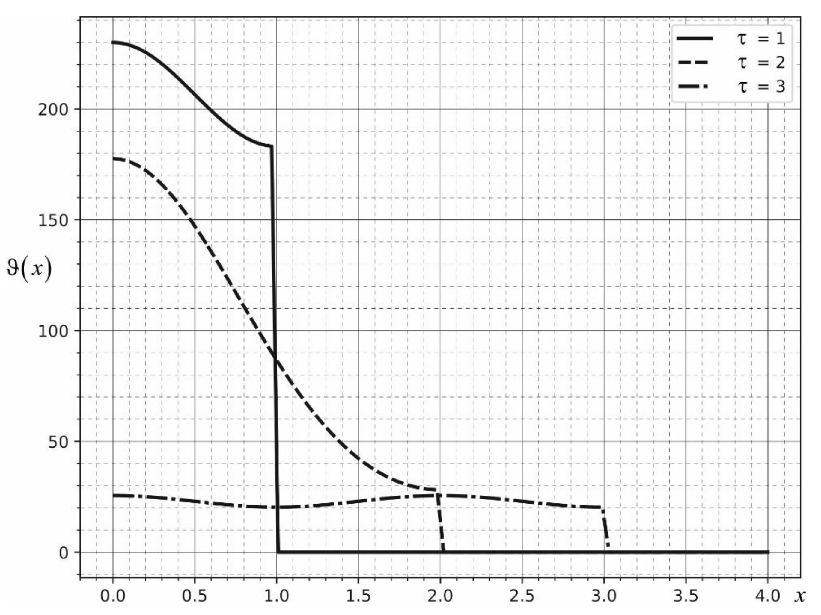
Using the superposition principle [40,41,42,43] and the transient function (26), the solution of the problem of the heat flux $q\left(x,y\right)$ on the surface $z=0$ of the half-space can be represented in the integral form:

$$\mathsf{\vartheta }\left(x,y,z,\mathsf{\tau }\right)=G_f\ast q={\displaystyle \underset{0}{\overset{\mathsf{\tau }}{\int }}dt{\displaystyle \underset{-\infty }{\overset{\infty }{\int }}{\displaystyle \underset{-\infty }{\overset{\infty }{\int }}{G}_f\left(x-\mathsf{\xi },y-\mathsf{\zeta },z,\mathsf{\tau }-t\right)q\left(\mathsf{\xi },\mathsf{\zeta }\right)d\mathsf{\xi }d\mathsf{\zeta }}}}.$$

(28)

The symbol «$\ast$» denotes the convolution of functions in terms of spatial variables $x$, $y$ and time $\mathsf{\tau }$.

To substantiate Formula (28), we consider the initial-boundary value problem for the influence function

$${\ddot{G}}_f+{\dot{G}}_f=\Delta G_f, {\left.-\frac{\partial G_f}{\partial z}\right|}_{z=0}=\mathsf{\delta }\left(x,y\right)\mathsf{\delta }\left(\mathsf{\tau }\right), {\left.G_f\right|}_{\mathsf{\tau }=0}={\left.{\dot{G}}_f\right|}_{\mathsf{\tau }=0}=0.$$

(29)

Performing a convolution operation on Equation (29) with the source function $q=q\left(x,y,\mathsf{\tau }\right)$ using the properties of the delta function and the convolution differentiation operations:

$$\begin{gathered} {\ddot{G}}_f\ast q=G_f\ast \ddot{q}=\frac{{\partial }^2}{{\partial }^2\mathsf{\tau }}\left(G_f\ast q\right),{\dot{G}}_f\ast q=G_f\ast \dot{q}=\frac{\partial }{\partial }\left(G_f\ast q\right), \\ \Delta G_f\ast q=G_f\ast \Delta q=\Delta \left(G_f\ast q\right), \frac{\partial G_f}{\partial z}\ast q=G_f\ast \frac{\partial q}{\partial z}=\frac{\partial }{\partial z}\left(G_f\ast q\right), \\ \mathsf{\delta }\left(x,y\right)\mathsf{\delta }\left(\mathsf{\tau }\right)\ast q=q, \end{gathered}$$

we arrive at the problem

$$\ddot{\mathsf{\vartheta }}+\dot{\mathsf{\vartheta }}=\Delta \mathsf{\vartheta }, {\left.-\frac{\partial \mathsf{\vartheta }}{\partial z}\right|}_{z=0}=q\left(x,y,\mathsf{\tau }\right), {\left.\mathsf{\vartheta }\right|}_{\mathsf{\tau }=0}={\left.\dot{\mathsf{\vartheta }}\right|}_{\mathsf{\tau }=0}=0, \mathsf{\vartheta }=G_f\ast q,$$

(30)

which proves the validity of the integral representation Equation (28).

Let us now show that taking into account the structure of expressions for the transient function Equation (26) and the heat flow model Equation (27), the integrals over the spatial variables in Equation (28) are calculated analytically. To do this, consider an auxiliary integral of the form

$$J\left(x\right)={\displaystyle \underset{-\infty }{\overset{\infty }{\int }}{e}^{-i{p}_n\left(x-\mathsf{\xi }\right)}{e}^{-\frac{{\mathsf{\xi }}^2}{2{\mathsf{\sigma }}^2}}d\mathsf{\xi }}=e^{-\frac{{\mathsf{\sigma }}^2{p}_n^2}{2}}{e}^{-i{p}_{n}x}{\displaystyle \underset{-\infty }{\overset{\infty }{\int }}{e}^{-i\frac{1}{2{\mathsf{\sigma }}^2}{\left(\mathsf{\xi }-i{\mathsf{\sigma }}^2{p}_n\right)}^2}d\mathsf{\xi }}.$$

Taking into account the formula ${\displaystyle \underset{-\infty }{\overset{\infty }{\int }}{e}^{-a{\left(\mathsf{\xi }-b\right)}^2}d\mathsf{\xi }}=\frac{\sqrt{\pi }}{\sqrt{a}}$, $a>0$, the integral is written in the final form:

$$J\left(x\right)=\mathsf{\sigma }\sqrt{2\pi }{e}^{-\frac{{\mathsf{\sigma }}^2{p}_n^2}{2}}{e}^{-i{p}_{n}x}.$$

(31)

Taking into account Equations (26), (28) and (31), we obtain a formula for calculating the temperature distribution in a half-space from the action of a stationary surface heat source:

$$\begin{gathered} \mathsf{\vartheta }\left(x,y,z,\mathsf{\tau }\right)=\frac{Q}{4{\mathsf{\tau }}^2}\cdot {\displaystyle \sum _{n=-\infty }^{\infty }{\displaystyle \sum _{m=-\infty }^{\infty }{a}_{mn}\left(z,\mathsf{\tau }\right){\mathsf{\varphi }}_{nm}\left(x,y\right)}}, \\ {a}_{mn}\left(z,\mathsf{\tau }\right)={\displaystyle \underset{0}{\overset{\mathsf{\tau }}{\int }}{e}^{-\mathsf{\beta }\left(\mathsf{\tau }-t\right)}{F}_f^F\left(p_n,p_m,z,\mathsf{\tau }-t\right)dt}, {\mathsf{\varphi }}_{nm}\left(x,y\right)=e^{-\frac{{\mathsf{\sigma }}^2}{2}\left(p_n^2+p_m^2\right)}{e}^{-i{p}_{n}x}{e}^{-i{p}_{m}y}. \end{gathered}$$

(32)

In the case of a moving heat source, as follows from Equation (2), $q=q\left[\mathsf{\xi }-\mathsf{\phi }\left(t\right),\mathsf{\zeta }-\mathsf{\psi }\left(t\right)\right]=\frac{Q{e}^{-\frac{{\left[\mathsf{\xi }-\mathsf{\phi }\left(t\right)\right]}^2+{\left[\mathsf{\zeta }-\mathsf{\psi }\left(t\right)\right]}^2}{2{\mathsf{\sigma }}^2}}}{2\pi {\mathsf{\sigma }}^2}$. Then Formula (28) takes the form

$$\mathsf{\vartheta }\left(x,y,z,\mathsf{\tau }\right)={\displaystyle \underset{0}{\overset{\mathsf{\tau }}{\int }}dt{\displaystyle \underset{-\infty }{\overset{\infty }{\int }}{\displaystyle \underset{-\infty }{\overset{\infty }{\int }}{G}_f\left(x-\mathsf{\xi },y-\mathsf{\zeta },z,\mathsf{\tau }-t\right)q\left[\mathsf{\xi }-\mathsf{\phi }\left(t\right),\mathsf{\zeta }-\mathsf{\psi }\left(t\right)\right]d\mathsf{\xi }d\mathsf{\zeta }}}}.$$

(33)

In the double integral we make a change of variables $\mathsf{\xi }-\mathsf{\phi }\left(t\right)={\mathsf{\xi }}^{\prime }$, $\mathsf{\zeta }-\mathsf{\psi }\left(t\right)={\mathsf{\zeta }}^{\prime }$, then

$$\mathsf{\vartheta }\left(x,y,z,\mathsf{\tau }\right)={\displaystyle \underset{0}{\overset{\mathsf{\tau }}{\int }}dt{\displaystyle \underset{-\infty }{\overset{\infty }{\int }}{\displaystyle \underset{-\infty }{\overset{\infty }{\int }}{G}_f\left(x-\mathsf{\phi }\left(t\right)-{\mathsf{\xi }}^{\prime },y-\mathsf{\psi }\left(t\right)-{\mathsf{\zeta }}^{\prime },z,\mathsf{\tau }-t\right)q\left({\mathsf{\xi }}^{\prime },{\mathsf{\zeta }}^{\prime }\right)d{\mathsf{\xi }}^{\prime }d{\mathsf{\zeta }}^{\prime }}}}.$$

(34)

The last expression, taking into account transformations similar to those made earlier, is reduced to the following calculation formula

$$\begin{gathered} \mathsf{\vartheta }\left(x,y,z,\mathsf{\tau }\right)=\frac{Q}{4{\mathsf{\tau }}^2}\cdot {\displaystyle \sum _{n=-\infty }^{\infty }{\displaystyle \sum _{m=-\infty }^{\infty }{a}_{mn}\left(z,\mathsf{\tau }\right){\mathsf{\varphi }}_{nm}\left(x,y\right)}}, \\ {a}_{mn}\left(z,\mathsf{\tau }\right)={\displaystyle \underset{0}{\overset{\mathsf{\tau }}{\int }}{e}^{-\mathsf{\beta }\left(\mathsf{\tau }-t\right)+i\left[p_n\mathsf{\phi }\left(t\right)+p_m\mathsf{\psi }\left(t\right)\right]}{F}_f^F\left(p_n,p_m,z,\mathsf{\tau }-t\right)dt}. \end{gathered}$$

(35)

In practical calculations, one should limit oneself to the number of members of the series in expressions Equation (32) or (35) sufficient to ensure the required accuracy:

$$\mathsf{\vartheta }\left(x,y,z,\mathsf{\tau }\right)\approx {\mathsf{\vartheta }}^N\left(x,y,z,\mathsf{\tau }\right)=\frac{Q}{4{\mathsf{\tau }}^2}\cdot {\displaystyle \sum _{n=-N}^N{\displaystyle \sum _{m=-N}^N{a}_{mn}\left(z,\mathsf{\tau }\right){\mathsf{\varphi }}_{nm}\left(x,y\right)}}.$$

(36)

Time integration in Formula (35) was carried out numerically using the adaptive Gauss–Kronrod method of the Python quadpy standard library [47].

6. Results

Figure 4 shows the function $\mathsf{\vartheta }\left(x,y,z,\mathsf{\tau }\right)$ at different points of the surface $z=0$ from time. The solid curve corresponds to the function $\mathsf{\vartheta }\left(0,0,0,\mathsf{\tau }\right)$, the dashed curve corresponds to the function $\mathsf{\vartheta }\left(3,0,0,\mathsf{\tau }\right)$, the dashed line corresponds to the function $\mathsf{\vartheta }\left(5,0,0,\mathsf{\tau }\right)$. It can be seen that until the arrival of the heat wave front, the temperature at the surface point does not change. The source is assumed stationary, located in the center of the coordinate system. The power of the source $Q=350$.

Figure 5 shows the distribution of the function $\mathsf{\vartheta }\left(x,y,z,\mathsf{\tau }\right)$ at the points of the surface $z=0$ along the coordinate $x$ at various points in time. The solid curve corresponds to the function $\mathsf{\vartheta }\left(x,0,0,1\right)$, the dashed curve corresponds to $\mathsf{\vartheta }\left(x,0,0,2\right)$, and the dash-dotted curve corresponds to $\mathsf{\vartheta }\left(x,0,0,3\right)$. The source is assumed to be stationary, located in the center of the coordinate system. Source power $Q=350$. The temperature wave propagation front is also clearly visible here.

Figure 6 shows the distribution of the function $\mathsf{\vartheta }\left(x,y,z,\mathsf{\tau }\right)$ along the coordinate $z$ at various points of time. The solid curve corresponds to the function $\mathsf{\vartheta }\left(0,0,z,1\right)$, the dashed curve corresponds to $\mathsf{\vartheta }\left(0,0,z,2\right)$, and the dash-dotted curve corresponds to $\mathsf{\vartheta }\left(0,0,z,3\right)$. The source is assumed to be stationary, located in the center of the coordinate system. Source power $Q=350$.

7. Conclusions

A numerical–analytical model was developed to determine the temperature field arising in the process of selective laser melting. A three-dimensional transient problem of the impact of a heat flux source on the surface of a half-space is solved using the superposition principle and the method of influence functions. The solution is built in quadratures. The kernel of the corresponding integral operator is the transient function of the surface heat source, constructed using the Fourier and Laplace integral transforms. This mathematical model allows one to determine the temperature distribution not only in the vicinity of the heating spot on the surface of the half-space, but also in depth, which is important in modeling 3D printing processes, as well as in studying heat transfer processes in materials exposed to high-enthalpy gas flows (for example, in conditions of aerogasdynamic flow around and heating of parts and assemblies of high-speed aircraft).

References

1. Biot, M. Thermoelasticity and Irreversible Thermodynamics. J. Appl. Phys. 1956, 27, 240–253. [Google Scholar] [CrossRef]
2. Lord, H.W.; Shulman, Y. A Generalized dynamical theory of thermoelasticity. J. Mech. Phys. Solids 1967, 15, 299–309. [Google Scholar] [CrossRef]
3. Green, A.E.; Lindsay, K.A. Thermoelasticity. J. Elast. 1972, 2, 1–7. [Google Scholar] [CrossRef]
4. Green, A.; Naghdi, P. A re-examination of the basic postulates of thermomechanics. Proc. R. Soc. Lond. A 1991, 432, 171–194. [Google Scholar]
5. Green, A.; Naghdi, P. Thermoelasticity without energy dissipation. J. Elast. 1993, 31, 189–208. [Google Scholar] [CrossRef]
6. Quintanilla, R. Moore-Gibson-Thompson Thermoelasticity. Math. Mech. Solids 2019, 24, 4020–4031. [Google Scholar] [CrossRef]
7. Quintanilla, R. Moore-Gibson-Thompson Thermoelasticity with two temperatures. Appl. Eng. Sci. 2020, 1, 100006. [Google Scholar] [CrossRef]
8. Thompson, P. Compressible-Fluid Dynamics; McGraw-Hill: New York, NY, USA, 1972. [Google Scholar]
9. Starovoitov, E.I.; Leonenko, D.V.; Orekhov, A.A. Bending of an elastoplastic circular sandwich plate on an elastic foundation in a temperature field. INCAS Bull. 2021, 13, 233–244. [Google Scholar] [CrossRef]
10. Starovoitov, E.I.; Leonenko, D.V.; Orekhov, A.A. Dynamic behavior of thin-walled elements of aircraft made of composite materials, excited by heat shock. J. Appl. Eng. Sci. 2020, 18, 724–731. [Google Scholar] [CrossRef]
11. Tushavina, O.V. Coupled heat transfer between a viscous shock gasdynamic layer and a transversely streamlined anisotropic half-space. INCAS Bull. 2020, 12, 211–220. [Google Scholar] [CrossRef]
12. Tushavina, O.V.; Kriven, G.I.; Hein, T.Z. Study of thermophysical properties of polymer materials enhanced by nanosized particles. Int. J. Circuits Syst. Signal Processing 2021, 15, 1436–1442. [Google Scholar] [CrossRef]
13. Abouelregal, A.; Alesemi, M.; Alfadil, H. Thermoelastic reactions in a long and thin flexible viscoelastic cylinder due to non-uniform heat flow under the non-Fourier model with fractional derivative of two different orders. AIMS Math. 2022, 7, 8510–8533. [Google Scholar] [CrossRef]
14. Abouelregal, A.E. Response of thermoelastic cylindrical cavity in a non-local infinite medium due to a varying heat source. Waves Random Complex Media 2020, 32, 1725–1742. [Google Scholar] [CrossRef]
15. Abouelregal, A.E.; Khalil, K.M.; Mohammed, W.W.; Atta, D. Thermal vibration in rotating nanobeams with temperature-dependent due to exposure to laser irradiation. AIMS Math. 2022, 7, 6128–6152. [Google Scholar] [CrossRef]
16. Abouelregal, A.E.; Mohammad-Sedighi, H.; Shirazi, A.H.; Malikan, M.; Eremeyev, V.A. Computational analysis of an infinite magneto-thermoelastic solid periodically dispersed with varying heat flow based on non-local Moore–Gibson–Thompson approach. Contin. Mech. Thermodyn. 2021, 34, 1067–1085. [Google Scholar] [CrossRef]
17. Biswas, S. Fundamental solution of steady oscillations equations in nonlocal thermoelastic medium with voids. J. Therm. Stresses 2020, 43, 284–304. [Google Scholar] [CrossRef]
18. Biswas, S. Three-dimensional nonlocal thermoelasticity in orthotropic medium based on Eringen’s nonlocal elasticity. Waves Random Complex Media 2022, 32, 1128–1149. [Google Scholar] [CrossRef]
19. Das, N.; De, S.; Sarkar, N. Reflection of plane waves in generalized thermoelasticity of type III with nonlocal effect. Math. Methods Appl. Sci. 2020, 43, 1313–1336. [Google Scholar] [CrossRef]
20. Sarkar, N.; Mondal, S.; Othman, M.I.A. Effect of the laser pulse on transient waves in a non-local thermoelastic medium under Green-Naghdi theory. Struct. Eng. Mech. 2020, 74, 471–479. [Google Scholar] [CrossRef]
21. Zhao, X.; Zhu, W.D.; Li, Y.H. Analytical solutions of nonlocal coupled thermoelastic forced vibrations of micro-/nano-beams by means of Green’s functions. J. Sound Vib. 2020, 481, 115407. [Google Scholar] [CrossRef]
22. Sarkar, N.; Bachher, M.; Das, N.; De, S.; Sarkar, N. Waves in nonlocal thermoelastic solids of type III. ZAMM Z. Fur Angew. Math. Und Mech. 2020, 100, e201900074. [Google Scholar] [CrossRef]
23. Deng, W.; Li, L.; Hu, Y.; Wang, X.; Li, X. Thermoelastic damping of graphene nanobeams by considering the size effects of nanostructure and heat conduction. J. Therm. Stresses 2018, 41, 1182–1200. [Google Scholar] [CrossRef]
24. Huang, M.; Wei, P.; Zhao, L.; Li, Y. Multiple fields coupled elastic flexural waves in the thermoelastic semiconductor microbeam with consideration of small scale effects. Compos. Struct. 2021, 270, 114104. [Google Scholar] [CrossRef]
25. Huang, Y.; Wei, P. Modelling the flexural waves in a nanoplate based on the fractional order nonlocal strain gradient elasticity and thermoelasticity. Compos. Struct. 2021, 266, 113793. [Google Scholar] [CrossRef]
26. Po, G.; Admal, N.C.; Svendsen, B. Non-local Thermoelasticity Based on Equilibrium Statistical Thermodynamics. J. Elast. 2020, 139, 37–59. [Google Scholar] [CrossRef]
27. Ge, X.; Li, P.; Fang, Y.; Yang, L. Thermoelastic damping in rectangular microplate/nanoplate resonators based on modified nonlocal strain gradient theory and nonlocal heat conductive law. J. Therm. Stresses 2021, 44, 690–714. [Google Scholar] [CrossRef]
28. Kumar, H.; Mukhopadhyay, S. Surface energy effects on thermoelastic vibration of nanomechanical systems under Moore–Gibson–Thompson thermoelasticity and Eringen’s nonlocal elasticity theories. Eur. J. Mech. A/Solids 2022, 93, 104530. [Google Scholar] [CrossRef]
29. Mohammed, W.W.; Abouelregal, A.E.; Atta, D.; Khelifi, F. Thermoelastic responses in a nonlocal infinite solid with a circular cylindrical cavity due to a moving heat supply under the MGT model of thermal conductivity. Phys. Scr. 2022, 97, 035705. [Google Scholar] [CrossRef]
30. Belov, P.A.; Lurie, S.A.; Dobryanskiy, V.N. Variational Formulation of Linear Equations of Coupled Thermohydrodynamics and Heat Conductivity. Lobachevskii J. Math. 2020, 41, 1949–1963. [Google Scholar] [CrossRef]
31. Lomakin, E.V.; Lurie, S.A.; Belov, P.A.; Rabinskiy, L.N. On the Generalized Heat Conduction Laws in the Reversible Thermodynamics of a Continuous Medium. Dokl. Phys. 2018, 63, 503–507. [Google Scholar] [CrossRef]
32. Lurie, S.A.; Belov, P.A. On the nature of the relaxation time, the Maxwell–Cattaneo and Fourier law in the thermodynamics of a continuous medium, and the scale effects in thermal conductivity . Contin. Mech. Thermodyn. 2020, 32, 503–507. [Google Scholar] [CrossRef]
33. Lurie, S.A.; Belov, P.A.; Volkov-Bogorodskii, D.B. Variational models of coupled gradient thermoelasticity and thermal conductivity. Mater. Phys. Mech. 2019, 42, 564–581. [Google Scholar] [CrossRef]
34. Zhang, K.Z.; AliShah, N.; Vieru, D.; El-Zahar, E.R. Memory effects on conjugate buoyant convective transport of nanofluids in annular geometry: A generalized Cattaneo law of thermal flux. Int. Commun. Heat and Mass Transf. 2022, 135, 106138. [Google Scholar] [CrossRef]
35. Bég, O.A.; Venkatadri, K.; Prasad, V.; Bég, T.; Leonard, H.J.; Gorla, R.; Rajarajeswari, P. Numerical study of magnetohydrodynamic natural convection in a non-Darcian porous enclosure filled with electrically conducting helium gas. Proc. Inst. Mech. Eng. Part C J. Mech. Eng. Sci. 2022, 236, 2203–2223. [Google Scholar] [CrossRef]
36. Cataneo, C.A. Form of heat conduction equation which eliminates the paradox of instantaneous propagation. Compte. Rendus. 1958, 247, 431–4433. [Google Scholar]
37. Vernotte, P. Les paradoxes de la theorie continue de lequation de la chaleur. CR Acad. Sci. 1958, 246, 3154–31555. [Google Scholar]
38. Lykov, A. Teoriya Teploprovodnosti; Vysshaya Shkola: Moscow, Russia, 1967. [Google Scholar]
39. Ditkin, V.; Prudnikov, A. Handbook on Operational Calculation; Vysshaya Shkola: Moscow, Russia, 1965. [Google Scholar]
40. Okonechnikov, A.; Tarlakovsky, D.; Fedotenkov, G. Spatial Non-Stationary Contact Problem for a Cylindrical Shell And Absolutely Rigid Body. Mech. Solids 2020, 55, 366–376. [Google Scholar] [CrossRef]
41. Serdyuk, A.; Serdyuk, D.; Fedotenkov, G. Stress-strain state of a composite plate under the action of a transient movable load. Mech. Compos. Mater. 2021, 57, 493–502. [Google Scholar] [CrossRef]
42. Fedotenkov, G.; Gritskov, A.; Levitskiy, D.; Vahterova, Y.; Sun, Y. Timoshenko beam and plate non-stationary vibrations. INCAS Bull. 2021, 13, 41–56. [Google Scholar] [CrossRef]
43. Serdyuk, A.; Serdyuk, D.; Fedotenkov, G. Unsteady bending function for an unlimited anisotropic plate. J. Samara State Tech. Univ. Ser. Phys. Math. Sci. 2021, 25, 111–126. [Google Scholar] [CrossRef]
44. Orekhov, A.; Rabinskiy, L.; Fedotenkov, G. Analytical Model of Heating an Isotropic Half-Space by a Moving Laser Source with a Gaussian Distribution. Symmetry 2022, 14, 650. [Google Scholar] [CrossRef]
45. Orekhov, A.; Rabinskiy, L.; Fedotenkov, G.; Hein, T. Heating of a half-space by a moving thermal laser pulse source. Lobachevskii J. Math. 2021, 42, 1912–1919. [Google Scholar] [CrossRef]
46. Fedotenkov, G.V.; Tarlakovskii, D.V.; Mitin, A.Y. Transient spatial motion of cylindrical shell under influence of non–stationary pressure. In Proceedings of the Second International Conference on Theoretical, Applied and Experimental Mechanics, Structural Integrity. Corfu, Greece, 23–26 June 2019; Springer: Cham, Switzerland, 2019; pp. 264–269. [Google Scholar]
47. Title of Site. Available online: https://github.com/sigma-py/quadpy (accessed on 3 August 2022).
Figure 1. Heating of a half-space by a moving heat source.
Symmetry 14 01950 g001
Figure 2. The practical convergence of the results. The solid curve corresponds to N = 10 , the dashed curve corresponds to N = 15 , and the dash-dotted curve corresponds to N = 20 .
Symmetry 14 01950 g002
Figure 3. Comparison of the results with the classical theory of heat conduction. Solid curve corresponds to the found generalized influence function G f , and the dashed curve corresponds to the known fundamental solution of the classical heat equation G c .
Symmetry 14 01950 g003
Figure 4. Dependence of temperature on time at different points on the surface of the half-space.
Symmetry 14 01950 g004
Figure 5. Temperature distribution along the coordinate at different points in time.
Symmetry 14 01950 g005
Figure 6. Temperature distribution along the coordinate at different points of time.
Symmetry 14 01950 g006
Publisher’s Note: MDPI stays neutral with regard to jurisdictional claims in published maps and institutional affiliations.