
Basic Statistical Properties of the Knot Efficiency


Abstract
:1. Introduction
- Two randomly selected pieces of rope are picked. A knot is placed on the first rope segment and afterwards it is broken to get value X. A second rope segment is broken in a straight setup without placing a knot to get value Y. Knot efficiency is calculated as the ratio . The total number of performed measurements is 2.This basic approach is the most widely spread because it is simple, relatively fast, and inexpensive (only two pieces of rope need to be destroyed). However, at the same time, results are significantly dependent on rope segment selection because this strategy does not take heterogeneity of inspected rope into account. Risk of improper efficiency assessment is high. Although this may seem obvious for the educated reader, this is the most common mistake, widely spread across the vast majority of texts.
- A more advanced, but still incorrect approach is based on the following idea. Split a rope into segments (unfortunately both n and m are usually a small numbers). Place a particular knot on randomly picked n of them, and perform breaking strength measurements. Get the experimental outcomes and evaluate mean value , and sometimes also the variance is evaluated. Break the remaining m segments in a straight setup without placing a knot to get the set of values with mean value and variance . Evaluate the mean knot efficiency as the ratio . Variances are usually left aside as they are not recognised as being a useful piece of information.This concept is the second most widely spread and slightly better than the first one since it at least reflects the heterogenous nature of rope and it implicitly indicates that the author is familiar with the random nature of breaking strength. However, it remains incorrect even if x and y are independent, at least because it is easy to prove that [8].
- to derive the PDF of the knot efficiency in general (see Section 2.1);
- to derive the special case PDF of the knot efficiency when breaking strength of knotted and straight rope is normally distributed (see Section 2.2);
- to explore properties of (see Section 2.3);
- to find a simpler yet accurate approximation to a relatively complex function in order to make calculations less demanding. In addition, we aim to specify the field of application, advantages, and drawbacks (see Section 2.4).
2. Results
2.1. Probability Density Function of the Knot Efficiency in General
- ;
- .
2.2. Probability Density Function of the Knot Efficiency for Normally Distributed Breaking Strength
- 1.
- p is related to the probability of breaking strength X being a negative (nonphysical) number: ;
- 2.
- q is related to probability of breaking strength Y being a negative (nonphysical) number: ;
- 3.
- r is ratio of expected values .
2.3. Properties of Knot Efficiency PDF
- Knotted rope breaking strength PDF is parameterised by two parameters and straight rope breaking strength PDF by another two parameters . However, knot efficiency PDF is fully parameterised only by three parameters instead of four (see Theorem 3, Equation (24)). Other parameterisations employing another triplets of parameters are also possible.
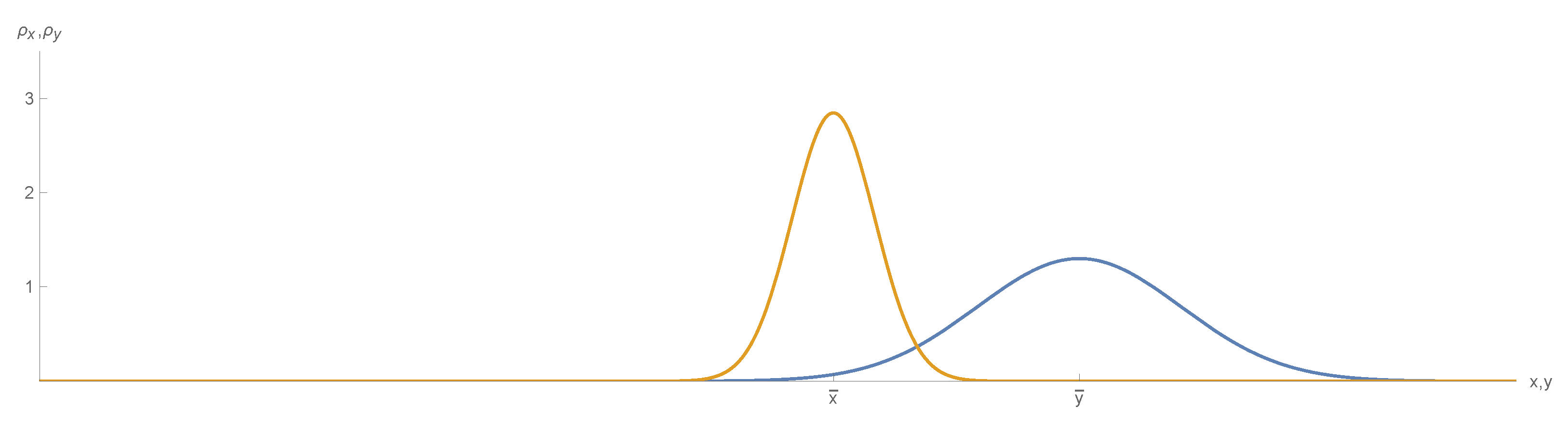
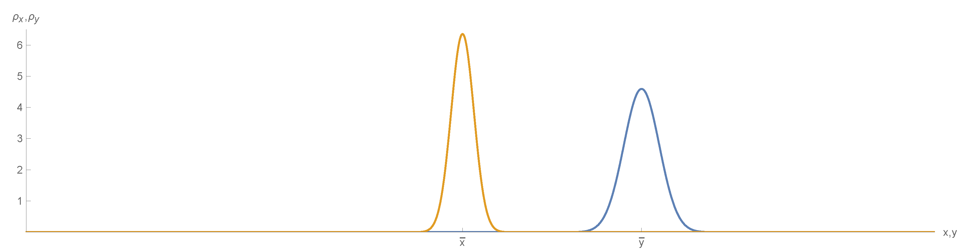
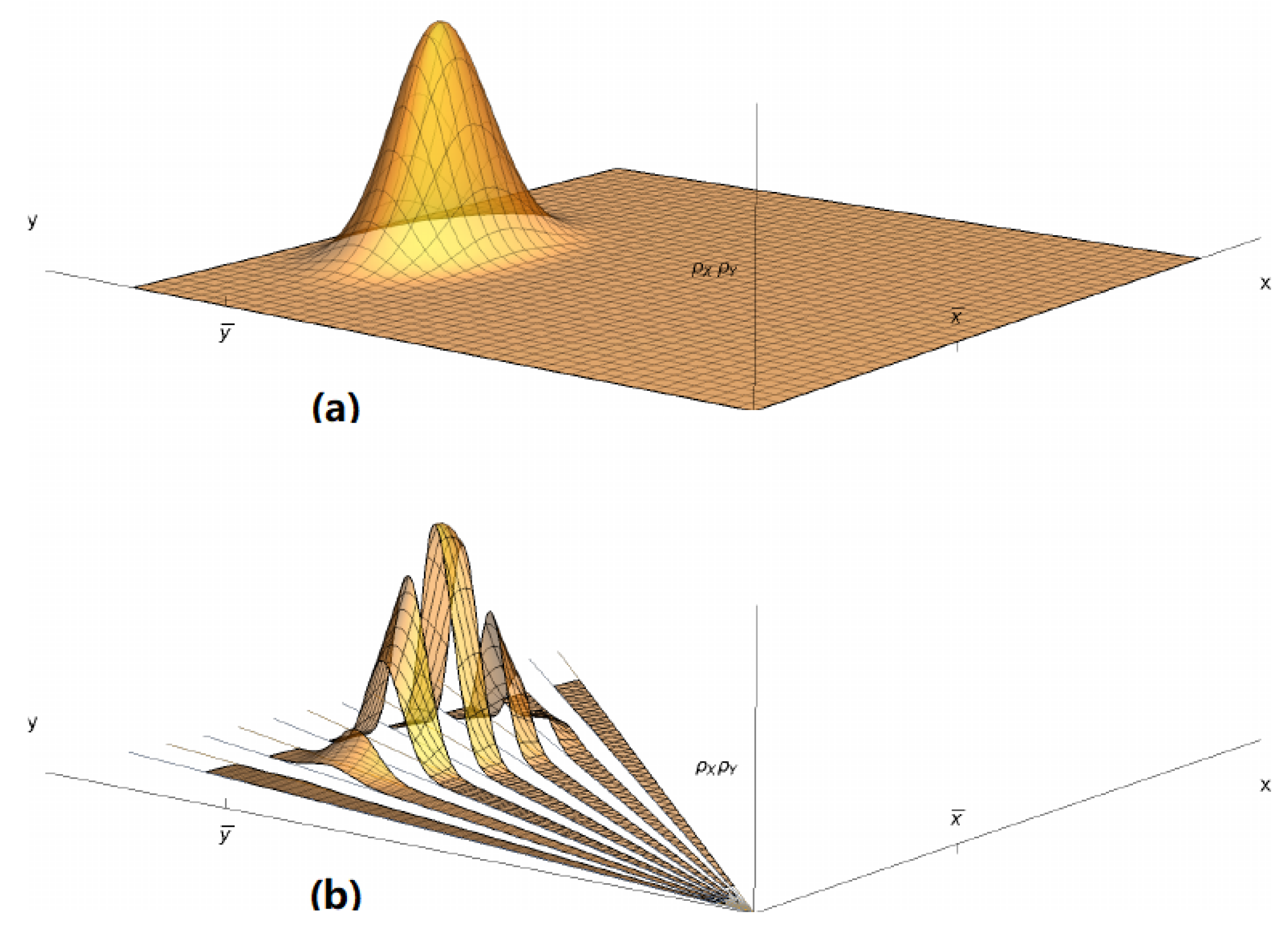
- Knot efficiency PDF is not a symmetric function under general reflection. Although it may seem symmetric upon first sight (see Figure 3a), it is important to stress that, depending on parameters it may be noticeably tailed or even bimodal. This is especially apparent if (see Figure 3b).In other words, for an arbitrary choice of parameters there does not exist such a point that would not change with respect to reflection over it:
- Cumulative distribution function of knot efficiency .Definition 7.Let be the knot efficiency PDF defined in Theorem 3 by Equation (24). Probability that knot efficiency η drawn from PDF is lower than is given by cumulative distribution functionFunction is continuous, non-decreasing (because ) and satisfies properties and . It can be used to calculate probability: . Unfortunately, it is not possible to express as a finite combination of elementary functions because integral does not have a closed-form solution. This is somewhat inconvenient because is essential to calculate probabilities, tolerance intervals, and quantiles. To evaluate any practical outcome, it is required to involve numerical methods. Another possibility is to use Hinkley’s formula [12] using so called Bivariate normal distribution function numerically tabulated by the National Bureau of Standards [29] or some of its approximations [30,31].
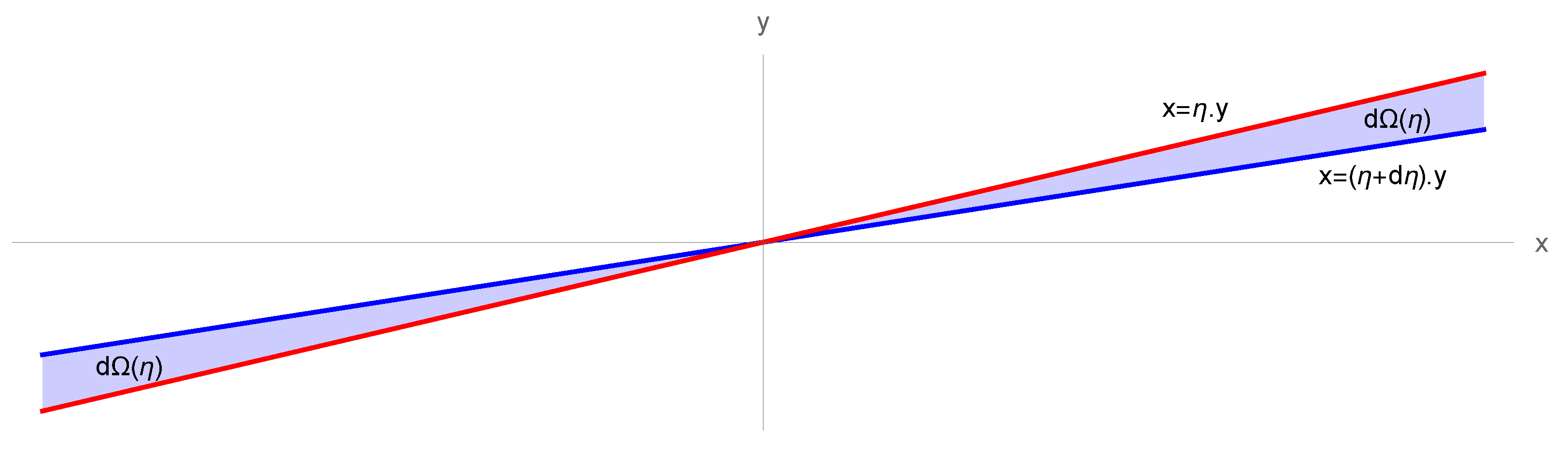
- An interesting feature of Equation (24) is that it entirely depends on argument . Ratio is also omnipresent across the whole body of . Let us call the quantity the relative knot efficiency and reserve symbol to label it. Substitution is directly coupled with related differential transformation . Probability must remain invariant under such a transformation, so the following equation holds true:Several new elements have been introduced to simplify the expressions so let us define them properly:Definition 8.Note that relative knot efficiency PDF is completely parameterised only by two parameters .Let us define a new dimensionless quantity and name it relative knot efficiency.
- Let be a new parameter. If , then parameter w falls into range ;
- PDF of relative knot efficiency is the function :
- cumulative distribution function of relative knot efficiency is the function :
- The relation between and is given by probability conservation principle. Equality of the following integrals is guaranteed , or:
- Probability that knot efficiency is a non-physical negative number is invariant of r and equals: . In order to become familiar with real knots values of , they have been calculated for selected combinations of parameters by means of numerical integration (see Table 2). It is clear that of real knots is negligibly small.
- Let and be non-negative integers. The probability that knot efficiency falls into range does not depend on r and equals:
- Knot efficiency PDF (see Equation (24)) does not have a finite mean or variance. It is a relatively easy task to prove that integrals and are divergent. Therefore, expected value is not finite (i.e., does not exist) and the same goes for variance [32,33].Moreover, real knots never break at negative breaking strength, and a knotted rope breaking higher than a straight one is extremely rare (to our knowledge it has never been reported yet). Function is continuous, non-negative, and bounded for . Therefore, it is well reasoned to calculate certainly finite mean and variance of truncated knot efficiency PDF, restricted on interval .Definition 9.Let ψ be the knot efficiency PDF and Ψ be the knot efficiency CDF introduced by Definition 7. Let ϕ be the solid approximation of relative knot efficiency PDF and Φ be the solid approximation of relative knot efficiency CDF introduced by Definition 8. Then, the expected value of knot efficiency on interval is defined by equation:Analogically, variance of knot efficiency on interval is defined by equation:To our knowledge, both and have to be evaluated by numerical integration techniques.
- In general, neither mode nor median shall be identified with ratio as one may intuitively suppose. The median knot efficiency can be evaluated only by means of numerical integration by solving integral equation orIt will be shown later in the text (see Theorem 5), that median and ratio of knot efficiency PDFs can be considered almost equal.
- PDF is in general bimodal [24], see Figure 3b. This means that it has two local maxima instead of one. According to numerical studies presented in [32], PDF is certainly bimodal if . If then the PDF may be either bimodal or unimodal, depending on the exact position of vector in the space of the parameters. There is a region separated from the rest of space by a simple curve such that for is unimodal. A good rule of thumb to make an accurate decision about PDF modality is to check the following two conditions:
- ;
- .
If both of them are satisfied simultaneously then knot efficiency PDF is almost certainly unimodal.However, one should keep in mind that the left modes of bimodal functions may be ignored in practical applications, as they are likely to occupy only a tiny fraction of the total area under the full density function, typically to or less [32].The mode of knot efficiency is the most likely value to be drawn from knot efficiency population. If the population PDF is continuously differentiable then the mode is a solution to the pair of conditions: - About of values drawn from a normal distribution are within one standard deviation away from the mean. This is a so-called tolerance interval well known in statistics, or . About of the values lie within two standard deviations and about within three standard deviations. For practical purposes, similar thresholds are also needed to be defined for knot efficiency PDF.
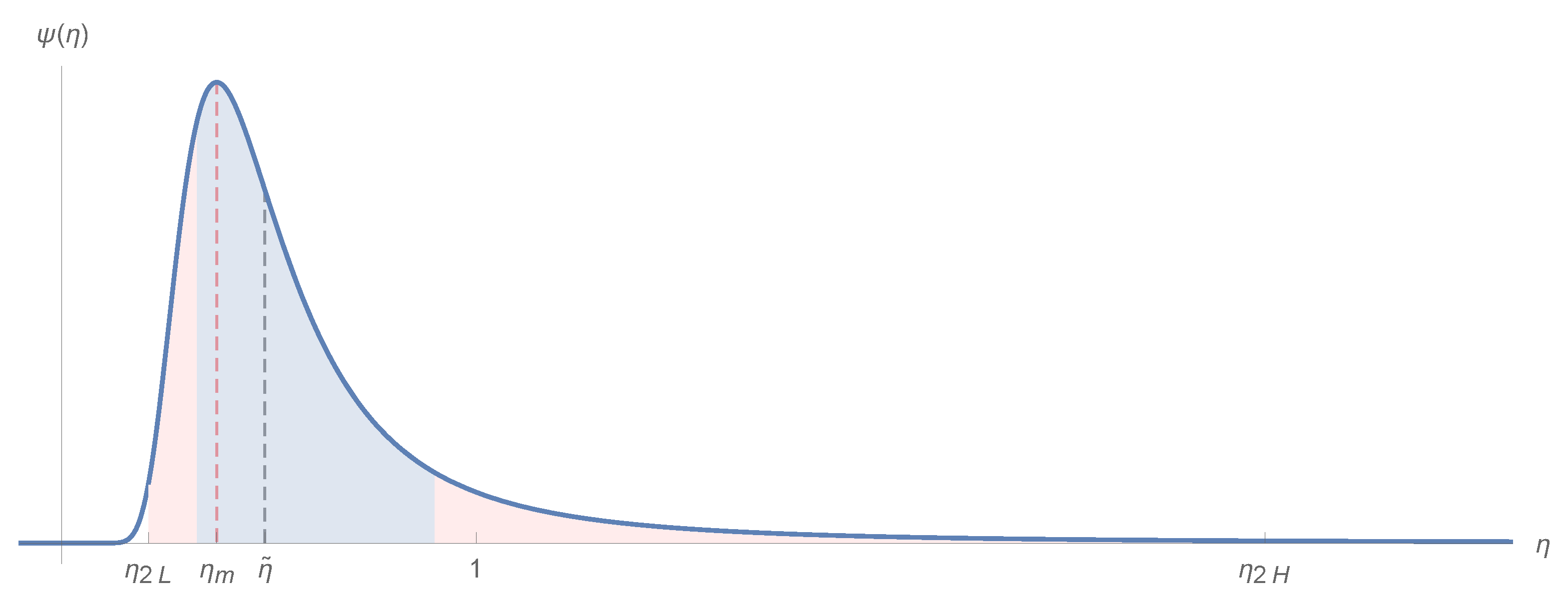
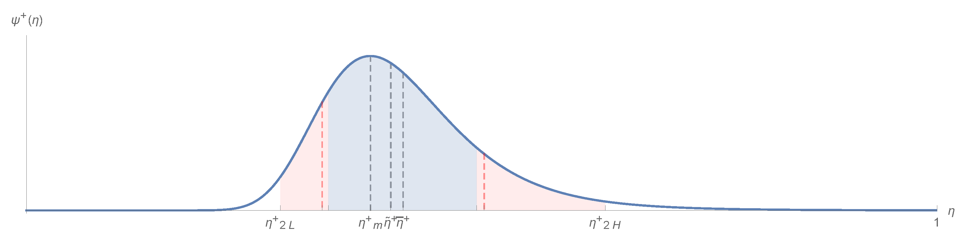
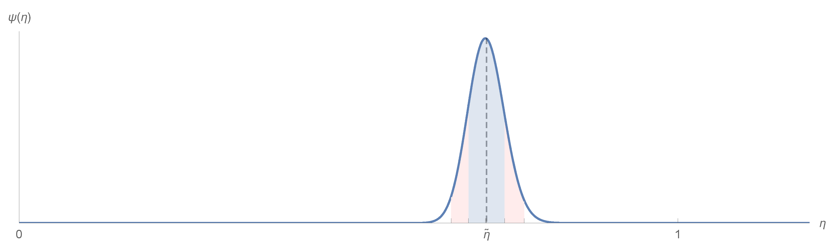
- Knot efficiency analogy to tolerance interval (see Figure 4) is . Thresholds have to meet pair of conditions: ;
- In general, knot efficiency analogy to interval for is . The following pair of conditions have to be fulfilled:Finding thresholds is subject to the numerical integration and depends on triplet of parameters or .
2.4. Solid Approximation to the Knot Efficiency PDF
- Parameters can be in general set to an arbitrary value. However, in the case of real knots, wide range is ruled out by laws of physics; hence, they will never be observed in real measurement. It has already been outlined in Assumption 1 that the vector of parameters always points into region for real data. Regarding the mentioned restrictions, function is bounded:
- Error function is monotonous increasing, as t increases asymptotically reaching . Hence, we are able to bound it:The lower bound of is for so close to the upper one, that with accuracy far beyond all practical needs we can simply write: ;
- Term is many orders of magnitude higher than than 1. Therefore, we can suppose:
- Concluding the above-mentioned reasoning, we are able to say:and after some algebraic manipulations we can proceed to approximationA similar equation can be written for the relative knot efficiency PDF:
- Both PDF formulae are less complex than ; hence, they are more suitable for practical calculations. Both of them are normalised, i.e., they obey integral relation . For any reasonable combination of parameters , solid approximation is indistinguishable from .
- Both CDFs and are closed-form formulae (see Definitions 10 and 11). Function is slightly simpler than so it is recommended to use it for calculations whenever possible. Relation holds true.
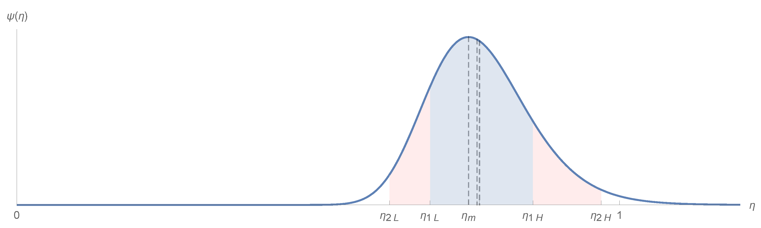
- Since is defined by explicit closed-form formula, median of solid approximation can be simply calculated by the following equation: .Theorem 5(Median ). Let be a solid approximation to relative knot efficiency CDF (see Definition 10). Then solid approximation to the median of knot efficiency is:Proof of Theorem 5.Median can be found from equation . According to Definition 10, it is possible to rewrite the equation:The solution is . □Position of the median is shown in the Figure 5.
- Solid approximation analogy to and tolerance interval can be found explicitly whenever condition is met. Solutions to equations and for are:
- interval:
- interval:
Ranges of and intervals are shown in the Figure 5 by colour shading.Note that and formulae are valid approximations if . Otherwise, more complex closed-form formulae containing inverse function can be easily derived. - It has already been stated that knot efficiency distributed by PDF does not have a finite mean or variance. Solid approximation itself does not bring any progress on this issue because PDF also leads to divergent integrals or . Nonetheless, truncated mean and variance can be calculated on the interval based on the same principles as Definition 9.
- Solid approximation to knot efficiency mean on the interval :
- Solid approximation to knot efficiency variance on the interval :
To our knowledge, both and have to be evaluated by numerical integration. Position of the truncated mean and standard deviation is shown in the Figure 5 by dotted lines.
2.5. Solid Approximation Error Management
- the absolute PDF error is defined by equation:
- the absolute CDF error is defined by equation:
- the absolute mean error is a constant defined by equation:
- the absolute variance error is a constant defined by equation:
- absolute difference of PDF functions is bounded for any :
- absolute difference of CDF functions is bounded for any :
3. Discussion
3.1. Figure Eight Loop Knot, Geometry O, Old Worn Rope
- Parameters are calculated according to Definitions 6 and 8:
- PDF function and CDF function are way too complicated. Let’s check whether using solid approximation counterparts would mean a significant accuracy issue or not.For the sake of appropriate accuracy mode selection, parameters and have to be evaluated firstly:According to Theorem 6, the absolute difference between CDF function and solid approximation counterpart for any is negligible:The same goes for absolute difference of truncated mean and variance calculated using solid approximation:Therefore, it is reasonable to use a wide spectrum of solid approximation advantages and keep results highly accurate at the same time.
- Statistical assessment of knot efficiency.
- -
- Probability density function
- -
- Cumulative distribution function
- -
- Median
- -
- ModeSolid approximation of knot efficiency PDF is a continuously differentiable function so the mode can be found by solving two conditions and . Numerical methods have been employed.
- -
- Truncated mean and variance
- -
- Tolerance intervalsAssumption has been met; therefore, solid approximation tolerance intervals and can be evaluated:
- -
- PDF graph (see Figure 7.)
- The most important conclusion is that knot efficiency is certainly not a sharp valued quantity. Truncated standard deviation is . Tolerance interval is wide and range is even wide. This is one of the reasons why it is so important to make as many breaking strength measurements on knotted and straight rope as possible.
- Niether tolerance intervals nor knot efficiency PDF are not symmetric, with a heavier tail on the right side. Any attempts to approximate this by normal distribution would result in misleading conclusions.
- There is a considerable probability to measure knot efficiency higher than . Namely, . This is not to be confused with truncated mean knot efficiency, median, or mode, which are well below 1 for any real knot.
- Mode, truncated mean and median are not the same number and it is important to decide which of these properties suit user purposes the best.
3.2. Figure Eight Loop Knot, Geometry O, New Rope
- Parameters are calculated according to Definitions 6 and 8:
- Let us check whether using solid approximation would mean a significant accuracy issue or not. For the sake of appropriate accuracy, mode selection parameters and have to be evaluated first:According to Theorem 6, the absolute difference between CDF function and solid approximation counterpart for any is negligible:The same goes for absolute difference of truncated mean and variance calculated using solid approximation:Therefore, it is reasonable to use a wide spectrum of solid approximation advantages and keep the results highly accurate at the same time. Moreover, in this particular case, even normal approximation would be accurate enough for .
- Statistical assessment of knot efficiency.
- -
- Probability density function
- -
- Cumulative distribution function
- -
- Median
- -
- ModeSolid approximation of knot efficiency PDF is a continuously differentiable function, the mode is a solution to relations and .
- -
- Truncated mean and variance
- -
- Tolerance intervalsAssumption has been met; therefore, solid approximation tolerance intervals and can be evaluated:
- -
- PDF graph (see Figure 9.)
- The knot efficiency of the same knot tied on the new rope is much better determined than in the previous example. Truncated standard deviation is approximately four times lower: . However, it is still not a sharp valued quantity.
- Tolerance interval is wide and range is wide. Tolerance intervals and knot efficiency PDF exhibit a high degree of symmetry. Mode, median, and truncated mean are very close to each other. There is high similarity with a normal distribution;
- Probability to measure knot efficiency from interval is negligible.
- Normal approximation is much easier to work with and it is recommended to use it if indicated [37]. In such a case mode, median and mean are considered to be the same value: , variance is given by simple explicit equation: . Note that the truncated solid approximation variance and normal approximation variance agree up to 5 decimal places in this particular example.
4. Conclusions
Author Contributions
Funding
Institutional Review Board Statement
Informed Consent Statement
Data Availability Statement
Acknowledgments
Conflicts of Interest
Abbreviations
| Probability density function; | |
| CDF | Cumulative distribution function; |
| Expected value of the random variable X; | |
| Variance of the random variable X; | |
| Normal distribution given by the mean and the variance ; | |
| Error function: . |
References
- Warner, C. Studies on the behaviour of knots. In History and Science of Knots; Turner, J.C., Griend, P., Eds.; World Scientific Publishing: Singapore, 1998; pp. 181–203. [Google Scholar]
- Šimon, J.; Dekýš, V.; Palček, P. Revision of Commonly Used Loop Knots Efficiencies. Acta Phys. Pol. A 2020, 138, 404–420. [Google Scholar] [CrossRef]
- Milne, K.A.; McLaren, A.J. An assessment of the strength of knots and splices used as eye terminations in a sailing environment. Sports Eng. 2006, 9, 1–13. [Google Scholar] [CrossRef]
- Marbach, G.; Tourte, B. Alpine Caving Techniques: A Complete Guide to Safe and Efficient Caving, 1st ed.; Speleo Projects: Allschwil, Switzerland, 2002; p. 71. [Google Scholar]
- Microys, H. Climbing Ropes. Am. Alpine J. 1977, 21, 137–147. [Google Scholar]
- McKently, J. Rescue knot efficiency revisited. Nylon Highw. 2014, 59, 1–4. [Google Scholar]
- Komorous, M. Connecting Knots and Their Influence on the Breaking Strength of Dynamic Rope. Bachelor’s Thesis, Charles University, Prague, Czech Republic, 2013. [Google Scholar]
- Montgomery, D.C.; Runger, G.C. Applied Statistics and Probability for Engineers, 3rd ed.; John Wiley & Sons: New York, NY, USA, 2003; pp. 157–188. [Google Scholar]
- Narula, S.C. The probability distribution of the ratio of the absolute values of two normal variables. J. Stat. Comput. Sim. 1989, 33, 173–182. [Google Scholar] [CrossRef]
- Geary, R.C. The frequency distribution of the quotient of two normal variates. J. R. Stat. Soc. 1930, 93, 442–446. [Google Scholar] [CrossRef]
- Curtiss, J.H. On the distribution of the quotient of two chance variables. Ann. Math. Stat. 1941, 12, 409–421. [Google Scholar] [CrossRef]
- Hinkley, D.V. On the ratio of two correlated normal variables. Biometrika 1969, 56, 635–639. [Google Scholar] [CrossRef]
- Deaton, L.W.; Kamerud, D.B. 6104: The Random Variable X/Y, X,Y Normal. Am. Math. Mon. 1978, 85, 206–207. [Google Scholar] [CrossRef]
- Shannon, C.E. A mathematical theory of communication. Bell. Syst. Tech. J. 1948, 27, 379–423. [Google Scholar] [CrossRef]
- Jaynes, E.T. Information Theory and Statistical Mechanics. Phys. Rew. 1957, 106, 620–630. [Google Scholar] [CrossRef]
- Cover, T.M.; Thomas, J.A. Elements of Information Theory, 2nd ed.; Wiley: New York, NY, USA, 1991; pp. 243–256. [Google Scholar]
- Grechuk, B.; Molyboha, A.; Zabarankin, M. Maximum Entropy Principle with General Deviation Measures. Math. Oper. Res. 2009, 34, 445–467. [Google Scholar] [CrossRef] [Green Version]
- Ross, S.M. Introductory Statistics, 4th ed.; Academic Press: Cambridge, MA, USA, 2017; pp. 297–328. [Google Scholar]
- Ross, S.M. Chapter 6—Distributions of sampling statistics. In Introduction to Probability and Statistics for Engineers and Scientists, 6th ed.; Ross, S.M., Ed.; Academic Press: Cambridge, MA, USA, 2021; pp. 221–244. [Google Scholar]
- Stover, C.; Weisstein, E.W. Closed-Form Solution. From MathWorld—A Wolfram Web Resource. Available online: https://mathworld.wolfram.com/Closed-FormSolution.html (accessed on 21 July 2022).
- Chow, T.Y. What is a closed-form number? Am. Math. Mon. 1999, 106, 440–448. [Google Scholar] [CrossRef]
- Marsaglia, G. Evaluating the normal distribution. J. Stat. Softw. 2004, 11, 1–11. [Google Scholar] [CrossRef]
- Fieller, E.C. The distribution of the index in a normal bivariate population. Biometrika 1932, 24, 428–440. [Google Scholar] [CrossRef]
- Marsaglia, G. Ratios of normal variables and ratios of sums of uniform variables. J. Am. Stat. Assoc. 1965, 60, 193–204. [Google Scholar] [CrossRef]
- Cedilnik, A.; Košmelj, K.; Blejec, A. The distribution of the ratio of jointly normal variables. Metod. Zv. 2004, 1, 99–108. [Google Scholar] [CrossRef]
- Nadarjah, S. Linear combination, product and ratio of normal and logistic random variables. Kybernetika 2005, 6, 787–798. [Google Scholar]
- Kuethe, D.O.; Caprihan, A.; Gach, H.M.; Lowe, I.J.; Fukushima, E. Imaging obstructed ventilation with NMR using inert fluorinated gases. J. Appl. Physiol. 2000, 88, 2279–2286. [Google Scholar] [CrossRef]
- Oliveira, A.; Oliveira, T.; Macías, S.A. Distribution function for the ratio of two normal random variables. In Proceedings of the International Conference on Numerical Analysis and Applied Mathematics 2014 (ICNAAM-2014), Rhodes, Greece, 22–28 September 2014. [Google Scholar]
- National Bureau of Standards. Tables of the Bivariate Normal Distribution Function and Related Functions, Applied Mathematics Series, 50; U.S. Government Printing Office: Washington, DC, USA, 1959; 258p.
- Cox, D.R.; Wermuth, N. A simple approximation for bivariate and trivariate normal integrals. Int. Stat. Rev. 1991, 59, 263–269. [Google Scholar] [CrossRef]
- Hong, H.P. An approximation to bivariate and trivariate normal integrals. Civ. Eng. Environ. Syst. 1999, 16, 115–127. [Google Scholar] [CrossRef]
- Marsaglia, G. Ratios of normal variables. J. Stat. Softw. 2006, 16, 1–10. [Google Scholar] [CrossRef]
- Frishman, F. On the arithmetic means and variances of products and ratios of random variables. In Statistical Distributions in Scientific Work; Patil, G.P., Kotz, S., Ord, J.K., Eds.; D. Reidel Publishing Company: Dordrecht, The Netherlands, 1975; pp. 401–406. [Google Scholar]
- Hass, J.R.; Heil, C. E; Weir, M.D. Thomas’ Calculus in SI units: Early transcendentals, 14th ed.; Pearson Education: Harlow, UK, 2019; p. AP-4. [Google Scholar]
- Merrill, A.S. Frequency distribution of an index when both the components follow the normal law. Biometrika 1928, 20A, 53–63. [Google Scholar] [CrossRef]
- Hayya, J.; Armstrong, D.; Gressis, N. A Note on the Ratio of Two Normally Distributed Variables. Manag. Sci. 1975, 21, 1338–1341. [Google Scholar] [CrossRef]
- Díaz-Francés, E.; Rubio, F.J. On the existence of a normal approximation to the distribution of the ratio of two independent normal random variables. Stat. Pap. 2013, 54, 309–323. [Google Scholar] [CrossRef]


| q | 1 | 2 | 3 | 4 | 5 |
| w = 0.2 | w = 0.3 | w = 0.4 | w = 0.5 | w = 0.6 | w = 0.7 | w = 0.8 | w = 0.9 | w = 1 | |
|---|---|---|---|---|---|---|---|---|---|
| q = 1 | |||||||||
| q = 2 | |||||||||
| q = 3 | |||||||||
| q = 4 | |||||||||
| q = 5 | |||||||||
| q = 6 | |||||||||
| q = 7 | |||||||||
| q = 8 | |||||||||
| q = 9 | |||||||||
| q = 10 |
Publisher’s Note: MDPI stays neutral with regard to jurisdictional claims in published maps and institutional affiliations. |
© 2022 by the authors. Licensee MDPI, Basel, Switzerland. This article is an open access article distributed under the terms and conditions of the Creative Commons Attribution (CC BY) license (https://creativecommons.org/licenses/by/4.0/).
Share and Cite
Šimon, J.; Ftorek, B. Basic Statistical Properties of the Knot Efficiency. Symmetry 2022, 14, 1926. https://doi.org/10.3390/sym14091926
Šimon J, Ftorek B. Basic Statistical Properties of the Knot Efficiency. Symmetry. 2022; 14(9):1926. https://doi.org/10.3390/sym14091926
Chicago/Turabian StyleŠimon, Ján, and Branislav Ftorek. 2022. "Basic Statistical Properties of the Knot Efficiency" Symmetry 14, no. 9: 1926. https://doi.org/10.3390/sym14091926
APA StyleŠimon, J., & Ftorek, B. (2022). Basic Statistical Properties of the Knot Efficiency. Symmetry, 14(9), 1926. https://doi.org/10.3390/sym14091926