Anti-Symmetric Medium Chirality Leading to Symmetric Field Helicity in Response to a Pair of Circularly Polarized Plane Waves in Counter-Propagating Configuration

Abstract

We examine how a chiral medium responds to a pair of plane waves of circular polarizations. To this goal, we assume the chiral medium to be spatially homogeneous for simplicity. By assuming the medium to be a lossless, we provide analytic formulas of key bilinear parameters such as the pair of electromagnetic and reactive Poynting vectors in addition to the pair of electromagnetic and reactive helicities. By examining two obliquely colliding plane waves, we learned that most of those key parameters are asymmetric with respect to the medium chirality. Only for a counter-propagating pair, some of those key parameters are found to exhibit symmetry with respect to the medium chirality. We will discuss the implications of those asymmetries and symmetries from the viewpoints of typical applications in optics and physics.

1. Introduction

From the viewpoint of light–matter interactions, optics consists of two components: optical media and electromagnetic (EM) waves [1,2,3]. As regards media, optical chirality is an anti-symmetric parameter, while a refractive index is normally a symmetric parameter. As regards EM waves, field helicity is one of the key characters in addition to the omni-important Poynting vector [3,4,5,6,7,8,9,10]. One is normally interested in how a media responds to an incident EM wave. We are here to examine such interactions in terms of symmetry and asymmetry (anti-symmetry being included) [2,11]. It is said in [12] that helical EM fields have long been exploited to characterize chiral matter (translated into our languages).

Before going deeper into chirality and helicity, both being the main topics of this study, let us consider electromagnetic antennas [13,14,15]. Even novices in engineering and technology have some experiences from their daily use of wireless cellular phones. A major function of antennas is to either receive or send EM signals, either from afar or out to far-away targets, respectively. However, ordinary users neglect the small antennas that are sitting within cellular phones. This is because the design of such mini antennas belongs to the job of engineers of commercial companies. Although the far-field behaviors are crucial to antennas considered as detectors [12], sensors [10], and communication gears, the near-field behaviors play important roles in properly designing antennas as electro-optic energy-conversion devices [14].

In this aspect, one could associate one pair of concepts, ‘active’ and ‘reactive’, with another pair of concepts, ‘radiating’ and ‘non-radiative’, respectively. The ‘reactive near field’ is defined as that region immediately surrounding an antenna wherein the reactive field predominates. In between this reactive near field and the ‘(Fraunhofer) far field’ lies the ‘radiating near field’, alternatively called either the ‘(Fresnel) intermediate field’ or the ‘transition field’. In comparison, this ‘reactive near field’ is alternatively called either the ‘nearest part of the near field’ or the ‘non-radiative near field. Meanwhile, consider a Mie scattering off a dielectric sphere illuminated by a plane wave. Here, the EM helicity is especially active in the near field, which arises from interactions among multiple scattered waves even if an external incident wave is linearly polarized [10,16]. As regards EM waves, both EM and reactive helicities make one of the key parameters in addition to the all-important Poynting vector.

With a firm grasp on the meaning of a near field obtained from the preceding paragraph, let us turn to another familiar phenomenon of light focusing. We observe that light focusing is normally accompanied by a spatially inhomogeneous EM field distribution [9,17]. For instance, the focal point is defined by the highest field intensity, while a focusing process is nothing but a process whereby EM energy is spatially intensified. Meanwhile, it is well-established that the angular momentum (AM) of an EM wave is decomposable into its spin and orbital parts [1,18,19,20]. Moreover, spatial alterations in an AM take place through a spatially inhomogeneous EM field, as either spin-to-orbital conversion (SOC) or orbital-to-spin conversion (OSC) [9,10]. In most cases, light focusing entails an OSC (not a SOC) as an EM wave progresses onto a near field (focal point) from a far field.

In our previous study in [16], we have shown that the EM field induced by an electric point dipole exhibits a SOC (not an OSC) from a near field (the dipole location) outwards into a far field. In other words, the spin AM is a near-field phenomenon, whereas the orbital AM is a far-field one from an approximate perspective. In short, a near-field spin AM and a far-field orbital AM prevail in an approximate sense [15]. From another viewpoint, either SOC or OSC takes place in the intermediate field [10]. Of course, a focusing process incurs a succession of varying polarization states [9]. In this study, the spin AM and polarization states will be handled in more detail. Other examples of light focusing are provided in various references of [16].

The constitutive relations for a chiral medium are odd in the chirality parameter of a medium. The resulting solutions to the governing Maxwell equations are thus largely odd in the chirality parameter. The asymmetry of such solutions is what has been conventionally found for the Mie scattering off a dielectric particle through an embedding chiral medium [21]. See Section 8.3 of [22] for details, where a pair of incident waves is employed in a collinear fashion. Recently, the same configuration is investigated with a view to how to enhance the usually weak chiral signals resulting from Mie scatterings [2]. The incident plane waves employed for such Mie scatterings are taken to be elliptically (circularly, included) polarized [16,23].

Two linearly polarized waves constitute an elliptically polarized incident wave. Two such elliptically polarized waves then undergo a co-propagation, namely, propagations in the same direction, although counter-rotations are implemented in the azimuthal direction [9,10,21,22,24,25]. Such a predominance of collinear incident waves led even to calling the co-propagation a ‘precondition’ for Mie scatterings [16,26,27]. Instead, we are interested in how a chiral medium responds to a pair of obliquely colliding plane waves [28,29,30].

Normally, various characteristics of a given EM field are probed by a foreign object immersed in that EM field. In this regard, opto-mechanical responses are utilized to examine the resulting light–matter interactions [3,9,16,19,20,27,31,32]. For instance, a foreign object could experience dilatation, rotation, or torsion due to the surrounding EM field [10,33].

For simplicity, we do not include any foreign objects within a medium, unlike scattering problems. The co-propagating pair and the counter-propagating (a.k.a. inversely propagating) pair will then be considered as two extreme cases by setting the oblique angle to zero and $\pi$, respectively, as sketched in Figure 1a [25,34]. Resultantly, a pair of obliquely colliding waves exhibit such an asymmetry prevailing in the key bilinear parameters [9,10]. What we found out is that the asymmetry turns into symmetry in the chirality parameter only in the rare configuration of two counter-propagating waves. Our system belongs to a type of extrinsic chiral system [26]. Although a pair of co-propagating waves can execute an (o-called simultaneous) oblique incidence on a space-fixed body [26], this configuration is not part of this study.

It is well known that distinct interference effects arise from interactions between a pair of obliquely colliding waves [4,34]. Counter-propagating pairs of beams are quite common in laser trapping [35], although beams of finite cross sections are employed in practical situations. For simplicity of analysis in this study, obliquely colliding plane waves are assumed of infinite extents. Notwithstanding, what makes our study non-simple is the fact that our pair of counter-propagating waves proceeds with wave numbers of different magnitudes because of medium chirality.

From a broader perspective, a generic set of multiple propagating waves should be treated in fully three-dimensional (3D) configurations. Depending on the relative orientations and polarization states of each constituent waves, numerous possibilities arise in terms of various interference effects [1,3,4,6,17,33]. As a special case, a pair of counter-propagating waves could form a standing wave, if the participating wave numbers are of an equal magnitude but of opposite signs [10,36]. Likewise, two crossed pairs of propagating waves could form two respective standing waves, when respective wave numbers in each pair are of equal magnitudes. Indeed, such two-pair standing waves are employed in 3D laser trapping [35].

The issue of symmetry is closely linked not only to geometry [9,11] but also to conservation laws [2,4,7,10,12,18,26,36]. By handling the Maxwell equations with necessary constitutive relations that reflect optical chirality, we can identify several EM parameters that characterize the EM fields: (i) a pair of energy densities (an EM energy density and an reactive energy density) [10,29,36,37], (ii) a pair of Poynting vectors (an EM Poynting vector and a reactive Poynting vector) [3,31,38], and (iii) a pair of field helicities (an EM helicity and a reactive helicity) [7,10,12,15,33]. These six parameters are bilinear in the electric and magnetic fields, which in turn satisfy the linear Maxwell equations. Therefore, we are still solving linear problems in this study, unlike in fluid mechanics which generically carries nonlinearities due mainly to nonlinear convection [2,3,8,9,39,40,41]. Yet, all the physically meaningful quantities are related to those six bilinear parameters. In other words, our upcoming symmetry and nonlinearity arise from considering not nonlinear problems but bilinear physical parameters.

Among these six field properties, we do not even need to mention the importance of the EM energy density, the EM Poynting vector, and the EM helicity as the key field parameters [1]. Notwithstanding, the remaining three reactive properties (the reactive energy density, the reactive Poynting vector, and the reactive helicity) are receiving increasing attention these days although the reactive parameters are less well known than the EM parameters [7,32]. The reactive helicity is alternatively called a ‘magneto-electric’ energy density, [7,15,19,32]. A ‘helicity’ sometimes implies only the sign (i.e., handedness) of the field helicity employed in this study [1,2,7,10,17,28]. It is emphasized for this study that both helicities are the property of the EM fields, while optical chirality is a material property [7]. Numerical studies on the EM field around a 3D ferrite disk show that reactive parameters are indeed strongly localized in the near field of that disk [10].

In a first approximation, forces and/or torques exerted on a nano-object can be evaluated in the small-particle Rayleigh limit [3,7,17]. Normally, the gradient force due to the EM energy density and the radiation pressure due to the Poynting EM vector are dominant [4,6,35]. Magneto-electric nano-objects immersed in EM waves are influenced by both EM and reactive Poynting vectors, when both electric and magnetic polarizabilities of nano-objects contain absorptive components [1,4,6,7,10,19,32]. The photo-kinetic (PK) force exerted on a Rayleigh particle by the EM fields is succinctly expressed in [3] and by Equation (15) of [38]. See [31] as well. The consequential forces and torques exerted on polarizable particles depend not only on the field characters but also on the exact values of the complex particle polarizabilities. When judiciously exploited, the anti-symmetry of the optical chirality of a medium offers several opportunities for sensing [12,42] and enantiomeric separation [24,43].

In case with a Mie scattering off a chiral particle immersed in an achiral medium, the symmetry and/or asymmetry of various bilinear parameters have already been investigated [7]. We may touch upon some analogues found in fluid mechanics as regards vorticities, characteristics, transitions, etc., wherever appropriate [2,3,8,9,40,41].

This study proceeds in the following way. Section 2 provides governing relations and key parameters. Section 3 offers plane-wave solutions to obliquely colliding waves, which are followed by the evaluations of the above-mentioned six EM parameters. Section 4 presents numerical results on the parameter space focusing on symmetry issues. Section 5 examines additional bilinear parameters from different perspectives. Section 6 provides discussions, followed by the conclusion in Section 7.

2. Formulation

Let us start with the Maxwell equations of $\tilde{\nabla }\times \tilde{E}=-\partial \tilde{B}/\partial \tilde{t}$ and $\tilde{\nabla }\times \tilde{H}=\partial \tilde{D}/\partial \tilde{t}$ along with the Gauss laws $\tilde{\nabla }·D=0$ and $\tilde{\nabla }·\tilde{B}=0$. Hereinafter, the tilde denotes dimensional quantities. Likewise, the nabla operator $\tilde{\nabla }$ is working with the dimensional space variables, say, $\left\{\tilde{x},\tilde{y},\tilde{z}\right\}$ in the Cartesian coordinates. Vectors should be formally written as the column vectors, say, ${\left\{\tilde{x},\tilde{y},\tilde{z}\right\}}^T$ with the superscript signifying ‘transpose’. However, to avoid confusion, note that $\left\{\tilde{x},\tilde{y},\tilde{z}\right\}$ is also employed.

Bold letters refer to vectors. The electric displacement $\tilde{D}$ and the magnetic induction $\tilde{B}$ are related to the electric field $\tilde{E}$ and the magnetic field $\tilde{H}$ through the pair of constitutive relations [22]. Here, $\tilde{\epsilon }$ and $\tilde{\mu }$ are the electric permittivity and the magnetic permeability, respectively. Furthermore, either $\tilde{\beta }$ or $\tilde{\kappa }$ is the chiral parameter as a material property of a medium. Hence, an optical medium under this study is characterized by the triad of either $\left\{\tilde{\epsilon },\tilde{\mu },\tilde{\beta }\right\}$ or $\left\{\tilde{\epsilon },\tilde{\mu },\tilde{\kappa }\right\}$, which are assumed spatially uniform for simplicity. Now, both fields of $\left\{\tilde{E},\tilde{H}\right\}$ are assumed to be time-oscillatory according to the temporal factor $\exp \left(-i\tilde{\omega }\tilde{t}\right)$, where $\left\{\tilde{\omega },\tilde{t}\right\}$ denote frequency and time.

Let us introduce the reference quantities: $\left\{{\tilde{\epsilon }}_0,{\tilde{\mu }}_0\right\}$, being equal to $\left\{\tilde{\epsilon },\tilde{\mu }\right\}$ evaluated in vacuum. In addition, ${\tilde{c}}_0={\left({\tilde{\epsilon }}_0{\tilde{\mu }}_0\right)}^{-1/2}$ is the light speed in vacuum, while ${\tilde{Z}}_0=\sqrt{{\tilde{\mu }}_0/{\tilde{\epsilon }}_0}$ is the impedance in vacuum [11]. Furthermore, we define the reference time $1/\tilde{\omega }$ and the reference wave number ${\tilde{k}}_0=\tilde{\omega }/{\tilde{c}}_0$. Here, $\tilde{\omega }$ is an assignable constant, for instance, in case with a monochromatic EM wave [7]. In brief,

$${\tilde{c}}_0\equiv \frac{1}{\sqrt{{\tilde{\epsilon }}_0{\tilde{\mu }}_0}},\begin{array}{c}\end{array}{\tilde{Z}}_0\equiv \sqrt{\frac{{\tilde{\mu }}_0}{{\tilde{\epsilon }}_0}},\begin{array}{c}\end{array}{\tilde{k}}_0=\frac{\tilde{\omega }}{{\tilde{c}}_0}$$

(1)

By use of these reference quantities, we define the following set of dimensionless parameters.

$$\begin{array}{l}\epsilon \equiv \frac{\tilde{\epsilon }}{{\tilde{\epsilon }}_0},\begin{array}{c}\end{array}\mu \equiv \frac{\tilde{\mu }}{{\tilde{\mu }}_0},\begin{array}{c}\end{array}\beta \equiv {\tilde{k}}_0\tilde{\beta },\begin{array}{c}\end{array}\kappa \equiv {\tilde{c}}_0\tilde{\kappa },\\ t\equiv \tilde{\omega }\tilde{t},\begin{array}{c}\end{array}\left\{x,y,z\right\}\equiv {\tilde{k}}_0\left\{\tilde{x},\tilde{y},\tilde{z}\right\},\begin{array}{c}\end{array}\nabla \equiv \frac{\tilde{\nabla }}{{\tilde{k}}_0},\\ E\equiv \frac{\tilde{E}}{{\tilde{E}}_0},\begin{array}{c}\end{array}H\equiv {\tilde{Z}}_0\frac{\tilde{H}}{{\tilde{E}}_0},\begin{array}{c}\end{array}D\equiv \frac{\tilde{D}}{{\tilde{\epsilon }}_0{\tilde{E}}_0},\begin{array}{c}\end{array}B\equiv {\tilde{Z}}_0\frac{\tilde{B}}{{\tilde{\mu }}_0{\tilde{E}}_0}\end{array}$$

(2)

Here, ${\tilde{E}}_0$ is an assignable reference electric field. Correspondingly, the dimensionless form of $\exp \left(-i\tilde{\omega }\tilde{t}\right)$ is the reduced factor $\exp \left(-it\right)$.

In this study, we will examine two types $\left\{C_{\beta }^{curl},C_{\kappa }^{field}\right\}$ of constitutive relations that are placed in the following dimensionless forms [21,22,27].

$$C_{\beta }^{curl}:\begin{array}{c}\end{array}\{\begin{array}{l}D=\epsilon \left(E+\beta \nabla \times E\right)\\ B=\mu \left(H+\beta \nabla \times H\right)\end{array};\begin{array}{c}\end{array}{C}_{\kappa }^{field}:\begin{array}{c}\end{array}\{\begin{array}{l}D=\epsilon E+i\kappa H\\ B=\mu H-i\kappa E\end{array}$$

(3)

For these dimensionless relations, we have started with the four dimensional relations $\tilde{D}=\tilde{\epsilon }\left(\tilde{E}+\tilde{\beta }\tilde{\nabla }\times \tilde{E}\right)$, etc. The first pair $C_{\beta }^{curl}$ is called the ‘curl-$\beta$-based constitutive relations’ [22]. In comparison, the second pair $C_{\kappa }^{field}$ is called the ‘field-$\kappa$-based constitutive relations’ [7,21,24,43]. This first pair is alternatively called the ‘Drude-Born-Fedorov relations’, while the second pair is called the ‘Tellegen relations’ [27,30]. Although $\kappa$ is complex for a generic Pasteur medium with $C_{\kappa }^{field}$ [28], we take $\kappa$ to be real in this study. Molecular implications of these chirality parameters are discussed by [24], where chiral impurities affecting the apparent chiral properties of water were taken as an example.

As intermediaries, let us introduce a pair $\left\{k_L,k_R\right\}$ of dimensionless wave numbers, respectively, for the two types of constitutive relations defined by Equation (3) [27].

$$\begin{array}{l}{C}_{\beta }^{curl}:\begin{array}{c}\end{array}\{\begin{array}{l}{k}_R\equiv \frac{\sqrt{\epsilon \mu }}{1+\beta \sqrt{\epsilon \mu }}\\ k_L\equiv \frac{\sqrt{\epsilon \mu }}{1-\beta \sqrt{\epsilon \mu }}\end{array},\begin{array}{c}\end{array}\beta \equiv \frac{1}{2}\left(\frac{1}{k_R}-\frac{1}{k_L}\right),\begin{array}{c}\end{array}\sqrt{\epsilon \mu }={\left[\frac{1}{2}\left(\frac{1}{k_R}+\frac{1}{k_L}\right)\right]}^{-1}\\ C_{\kappa }^{field}:\begin{array}{c}\end{array}\{\begin{array}{l}{k}_L\equiv \sqrt{\epsilon \mu }+\kappa \\ k_R\equiv \sqrt{\epsilon \mu }-\kappa \end{array}\end{array}$$

(4)

This pair $\left\{k_L,k_R\right\}$ will be derived later. Meanwhile, the Maxwell equations are transformed into the following dimensionless forms [22].

$$\{\begin{array}{l}\nabla \times E=iB\\ \nabla \times H=-iD\end{array},\begin{array}{c}\end{array}\{\begin{array}{l}\nabla ·E=0\\ \nabla ·H=0\end{array}$$

(5)

Our task with Equations (3) and (5) is to solve for the dimensionless field variables $\left\{E,H\right\}$ at the dimensionless space coordinate $\left\{x,y,z\right\}$ for the specified triad of either $\left\{\epsilon ,\mu ,\beta \right\}$ or $\left\{\epsilon ,\mu ,\kappa \right\}$ as dimensionless parameters.

Let us introduce a complex variable $f\equiv \mathrm{Re}\left(f\right)+i\mathrm{Im}\left(f\right)$ for any $f\in ℂ$ being complex, where the superscript $*$ denotes a complex conjugate. Let us define a pair of energy densities.

$$I\equiv \frac{1}{2}\left(\epsilon E^{*}·E+\mu H^{*}·H\right),\begin{array}{c}\end{array}J\equiv \frac{1}{2}\left(\epsilon E^{*}·E-\mu H^{*}·H\right)$$

(6)

Here, $\left\{I,J\right\}$ are the EM energy density and the reactive energy density, respectively. It is obvious that $I$ takes a form based on the electric-magnetic democracy (or duality) [10,18,20], namely, symmetric with respect to the interchange in $\left\{\epsilon E^{*}·E,\mu H^{*}·H\right\}$. $I$ is the positive definite for $\epsilon ,\mu >0$ [2]. In contrast, $J$ is of an anti-electric-magnetic democracy, i.e., inverting its sign with respect to the interchange in $\left\{\epsilon E^{*}·E,\mu H^{*}·H\right\}$.

Furthermore, we establish two pairs of complex parameters $E·H^{*}\equiv K+iC$ and $E\times H^{*}\equiv P+iR$ based on the field vectors $\left\{E,H\right\}$.

$$\{\begin{array}{l}P\equiv \mathrm{Re}\left(E\times H^{*}\right)\\ R\equiv \mathrm{Im}\left(E\times H^{*}\right)\end{array},\begin{array}{c}\end{array}\{\begin{array}{l}C\equiv \mathrm{Im}\left(E·H^{*}\right)\\ K\equiv \mathrm{Re}\left(E·H^{*}\right)\end{array}$$

(7)

Here, $\left\{P,R\right\}$ are the EM Poynting vector and the reactive Poynting vector, respectively. As the most important parameter in characterizing EM fields [5,20], the EM Poynting vector is alternatively called a ‘kinetic Abraham momentum density’ [18,27]. The EM Poynting vector is related to a radiation pressure exerted on nano-objects immersed in the EM fields [3,6]. In this connection, we remark that the scattering cross sections are evaluated based on the EM Poynting vector when it comes to Mie scatterings [21,22]. Meanwhile, the polarization states of EM fields are linked to $E·H^{*}\equiv K+iC$ [6].

In addition, $\left\{C,K\right\}$ are the EM helicity and the reactive helicity (densities), respectively [20,42,44]. We learn that $C$ is alternatively called an ‘active helicity’ [43], whereas $K$ is alternatively called a ‘active chirality’ or just a ‘chirality’ [7]. Since $\beta$ is dubbed an ‘optical chirality’ of a medium, we decided to intentionally call $\left\{C,K\right\}$ an ‘EM helicity’ and a ‘reactive helicity’, respectively, so as to differentiate them from the medium chirality, viz., either $\beta$ or $\kappa$.

Notice in Equation (2) that $\left\{\epsilon ,\mu \right\}$ denote a relative permittivity and a relative permeability, respectively. From here on, we assume a medium under consideration to be lossless so that $\left\{\epsilon ,\mu ,\beta ,\kappa \right\}$ are real for simplicity. In this study, we place a further restriction that $\epsilon ,\mu >0$. Hence, the conventional refractive index $n$ is given by $n\equiv \sqrt{\epsilon \mu }$ [1]. Consulting the constitutive relations in Equation (3), $C\equiv \mathrm{Im}\left(E·H^{*}\right)$ can be alternatively defined by $C\equiv \mathrm{Im}\left(D·B^{*}\right)$ [12]. This distinction between the two defining formulas for $C$ is essentially linked to the Abraham–Minkowski dilemma [18,27,45], details of which lie beyond the scope of this study.

We can invert the Maxwell equations in Equation (5) together with Equation (3) to obtain the matrix relation $\nabla \times {\left\{E,H\right\}}^T=K{\left\{E,H\right\}}^T$ with the interaction matrix $K$ defined below, differing according to the constitutive relations.

$$\nabla \times \left\{\begin{array}{c}E\\ H\end{array}\right\}=K\left\{\begin{array}{c}E\\ H\end{array}\right\},\begin{array}{c}\end{array}\{\begin{array}{l}{C}_{\beta }^{curl}:\begin{array}{c}\end{array}K\equiv \frac{1}{1-\epsilon \mu {\beta }^2}\left(\begin{array}{cc}\epsilon \mu \beta & i\mu \\ -i\epsilon & \epsilon \mu \beta \end{array}\right)\\ C_{\kappa }^{field}:\begin{array}{c}\end{array}K\equiv \left(\begin{array}{cc}\kappa & i\mu \\ -i\epsilon & \kappa \end{array}\right)\end{array}$$

(8)

It is implied by Equation (8) that one of $\left\{E,H\right\}$ is the vorticity of the other and vice versa [4], analogues of which are amply found in fluid mechanics [2,40]. A key point is the near-anti-symmetry of $K$ except for the distinct off-diagonal factors of $\left\{\epsilon ,\mu \right\}$. Both $K$-matrices in Equation (8) are of an identical structure. This aspect can be easily verified, say, for the second relation of Equation (8) in case with $C_{\kappa }^{field}$.

$$\left(\begin{array}{cc}\kappa & i\mu \\ -i\epsilon & \kappa \end{array}\right)=\kappa \left(\begin{array}{cc}1& 0\\ 0& 1\end{array}\right)+i\frac{1}{2}\left(\mu -\epsilon \right)\left(\begin{array}{cc}0& 1\\ 1& 0\end{array}\right)-\frac{1}{2}\left(\mu +\epsilon \right)\left(\begin{array}{cc}0& -i\\ i& 0\end{array}\right)$$

(9)

We have on the right-hand side of Equation (9) a pair $\left\{{\sigma }_1,{\sigma }_2\right\}$ of Pauli matrices. The first relation of Equation (8) in case with $C_{\beta }^{curl}$ can be understood in an analogous fashion. Among the three matrices on the right-hand side of Equation (9), the first diagonal matrix refers to a rate of stretching, while the second matrix implies a rate of shearing [3,28]. These two matrices are symmetric. In comparison, the third anti-symmetric matrix of Equation (9) signifies vorticity. The corresponding plane of rotation lies on the $xy$-plane as depicted in Figure 1. This vorticity is associated with a certain axial vector, which we choose to be directed along the $z$-coordinate in Figure 1. Linked to vortices, there are diverse phenomena such as toroidal rolls, rotating clouds, helical streamlines, etc. [3,8,10].

Let us introduce the following pairs of auxiliary vectors.

$$\{\begin{array}{l}{A}_{\pm }\equiv {\left[E^{*}·\left(\nabla \times H\right)\mp H^{*}·\left(\nabla \times E\right)\right]}^{*}\\ B_{\pm }\equiv \mu H^{*}·\left(\nabla \times H\right)\mp \epsilon E^{*}·\left(\nabla \times E\right)\end{array}$$

(10)

Let us form dot products such that the Faraday law $\nabla \times E=iB$ and the Ampère law $\nabla \times H=-iD$ both in (5) give rise to $H^{*}·\left(\nabla \times E\right)=i{H}^{*}·B$ and $E^{*}·\left(\nabla \times H\right)=-i{E}^{*}·D$. They are then denoted by $\left(FL\right)$ and $\left(AL\right)$, respectively. We then take the difference $\left(FL\right)-\left(AL\right)$ and the sum $\left(FL\right)+\left(AL\right)$, whence their respective real and imaginary parts are separated. In this manner, we obtain the following pair of conservation laws involving $\left\{\nabla ·P,\nabla ·R\right\}$ together with another pair of constraint relations [17,27,29,37].

$$C_{\beta }^{curl}:\begin{array}{c}\end{array}\{\begin{array}{l}\{\begin{array}{l}I=\frac{1}{2}\mathrm{Im}\left(A_{+}\right)-\frac{1}{2}\beta \mathrm{Re}\left(B_{-}\right)\\ \nabla ·P=-\frac{1}{2}\mathrm{Re}\left(A_{+}\right)-\frac{1}{2}\beta \mathrm{Im}\left(B_{-}\right)\end{array}\\ \{\begin{array}{l}J+\nabla ·R=-\frac{1}{2}\mathrm{Im}\left(A_{-}\right)+\frac{1}{2}\beta \mathrm{Re}\left(B_{+}\right)\\ \mathrm{Re}\left(A_{-}\right)+\beta \mathrm{Im}\left(B_{+}\right)=0\end{array}\end{array};\begin{array}{c}\end{array}{C}_{\kappa }^{field}:\begin{array}{c}\end{array}\{\begin{array}{l}\{\begin{array}{l}I=\frac{1}{2}\mathrm{Im}\left(A_{+}\right)-\kappa \mathrm{Im}\left(E·H^{*}\right)\\ \nabla ·P+\frac{1}{2}\mathrm{Re}\left(A_{+}\right)=0\end{array}\\ \{\begin{array}{l}J+\nabla ·R+\frac{1}{2}\mathrm{Im}\left(A_{-}\right)=0\\ \frac{1}{2}\mathrm{Re}\left(A_{-}\right)=\kappa \mathrm{Re}\left(E·H^{*}\right)\end{array}\end{array}$$

(11)

Here, we employed the two types of constitutive relations listed in Equation (3). This rather complicated set of relations in Equation (11) is reduced to a simpler set for an achiral medium. In this respect, Equations (3) and (5) are reduced to $\nabla \times E=i\mu H$ and $\nabla \times H=-i\epsilon E$ for an achiral medium with either $\beta =0$ or $\kappa =0$. Hence, Equation (10) is reduced to $\left\{A_{+},A_{-}\right\}=2i\left\{I,J\right\}$ and $B_{+}+B_{-}=-i2\epsilon \mu E·H^{*}$. For an achiral medium with $\beta =0$, especially for the curl-$\beta$-based constitutive relations, we have a more physically meaningful reduced pair of $B_{+}=-i2\epsilon \mu K$ and $B_{-}=2\epsilon \mu C$ as proved in Supplementary Material. Notice that $B_{+}=-i2\epsilon \mu K$ is linked to $R$ as seen from $J+\nabla ·R=-\frac{1}{2}\mathrm{Im}\left(A_{-}\right)+\frac{1}{2}\beta \mathrm{Re}\left(B_{+}\right)$ in Equation (11). For this reason, $\frac{1}{2}K$ is alternatively called a magneto-electric energy density [10].

For an achiral medium with either type of constitutive relations, the second relation of the first pair in Equation (11) is reduced to the familiar conservation law $\nabla ·P=0$, while the first relation of the second pair in Equation (11) is reduced to $\nabla ·R+2J=0$ [9,10]. In comparison, the remaining two relations in Equation (11) are trivially satisfied. The equations involving $\nabla ·P$ in the conservation laws of Equation (11) carry a non-conservative term $\mathrm{Re}\left(A_{-}\right)$, which cannot be expressed as a divergence of something such as $\nabla {\Phi }_{-}$ [6]. Likewise, the equations involving $\nabla ·R$ in the conservation laws of Equation (11) carry a non-conservative term $\mathrm{Re}\left(A_{+}\right)$, which cannot be expressed as a divergence of something such as $\nabla {\Phi }_{+}$ [6]. According to Equation (10), both of $\mathrm{Re}\left(A_{\pm }\right)$ account for curl components [4]. We will examine in the future the conditions under which $\frac{1}{2}\mathrm{Re}\left(A_{\pm }\right)$ can be expressed as divergences of scalar potentials ${\Phi }_{\pm }$, namely, in $\mathrm{Re}\left(A_{\pm }\right)=\nabla {\Phi }_{\pm }$.

Among many works on the conservation laws [2,4,7,26], details can be found in the Supplementary Material of [12], where lossy media are handled as well. Notwithstanding, we can hardly find conservation laws that explicitly involve $\beta$ or $\kappa$ as in Equation (11). In addition to Equation (11), we have placed in Supplementary Material other forms of $\left\{P,R\right\}$ that are of lesser utility to this study but warrant further investigations [1,2,3,4,12,18,20,43,44,45].

There are other set of chirality–helicity conservation laws that hold true between the pair $\left\{C,K\right\}$ of Equation (7) and the pair $\left\{E^{*}\times E,H^{*}\times H\right\}$. Consider the polarization states $\mathrm{Im}\left(E^{*}\times E\right)$ and $\mathrm{Im}\left(H^{*}\times H\right)$ in the physical $EH$-space [8]. We can then define the average spin angular momentum (AM) density $M\equiv \frac{1}{2}\mathrm{Im}\left(\epsilon E^{*}\times E+\mu H^{*}\times H\right)$ suitable for the electric-magnetic democracy. It is alternatively called a canonical spin angular momentum (AM) density [2,9,17,18]. As a counterpart to the energy conservation laws presented in Equation (11), we can then derive the chirality conservation law involving $\nabla ·M$ as easily proved in Supplementary Material.

$$M\equiv \frac{1}{2}\mathrm{Im}\left(\epsilon E^{*}\times E+\mu H^{*}\times H\right),\begin{array}{c}\end{array}\{\begin{array}{l}{C}_{\beta }^{curl}:\begin{array}{c}\end{array}\nabla ·M+\frac{2\epsilon \mu }{1-\epsilon \mu {\beta }^2}K=0\\ C_{\kappa }^{field}:\begin{array}{c}\end{array}\nabla ·M=0\end{array}$$

(12)

Our dimensionless scheme relying on Equations (1)–(3), (5)–(7) and (12) is consistent with the formulas of [20]. In addition, the average induced current $\nabla \times M$ is related to the spin part [18] as discussed in Supplementary Material. The curl $\nabla \times M$ is also related to the spin-curl forces [3,8,17].

Thanks to the cancellation by $\exp \left(-it\right)\exp \left(+it\right)=1$, the six parameters of Equations (6) and (7) as well as $M$ in Equation (12) are devoid of time dependence. For these seven parameters, we have neglected the factor of half arising from the time average of time-oscillatory parameters [33]. It is stressed that the seven parameters listed in Equations (6), (7), and (12) are bilinear (quadratic included) in the field variables $\left\{E,H\right\}$. Therefore, the linear properties $\left\{E,H\right\}$ are not directly transferred to these six bilinear parameters, which carry many interesting mathematically nonlinear properties.

For a generic EM wave with $\left\{E,H\right\}$, let us form the pair of spin angular momentum (AM) densities:$M_E\equiv \mathrm{Im}\left(\epsilon E^{*}\times E\right)$ (electric) and $M_H\equiv \mathrm{Im}\left(\epsilon H^{*}\times H\right)$ (magnetic). We then evaluate their respective spatial divergences $\left\{\nabla ·M_E,\nabla ·M_H\right\}$. It is well-known that $K\equiv \mathrm{Re}\left(E·H^{*}\right)$ is proportional to either of $\left\{\nabla ·M_E,\nabla ·M_H\right\}$. Meanwhile, the EM Poynting vector $P$ can be decomposed into its spin and orbital parts [1,18,19,20]. It is then easy to relate the spin part to the curl $\frac{1}{2}\nabla \times M_E$ (electric) and $\frac{1}{2}\nabla \times M_H$. These relations have been proven only for achiral media in [32,46]. Modified versions for chiral media should contain terms proportional to either of $\left\{\beta ,\kappa \right\}$ depending on the constitutive relations as in Equation (11). We leave that topic to another future work.

3. Plane-Wave Solutions for Obliquely Colliding Waves

The pair $\left\{E,H\right\}$ of vectors lies in the ‘physical $EH$-space’, which can be rewritten in terms of the pair $\left\{Q_L,Q_R\right\}$ of vectors in the ‘circular $Q$-space’. Both pairs are related through the following transformation rule.

$$\left\{\begin{array}{c}E\\ H\end{array}\right\}=A\left\{\begin{array}{c}{Q}_L\\ Q_R\end{array}\right\},\begin{array}{c}\end{array}Z\equiv \sqrt{\frac{\mu }{\epsilon }},\begin{array}{c}\end{array}A\equiv \left(\begin{array}{cc}1& -iZ\\ -i{Z}^{-1}& 1\end{array}\right)=\left(\begin{array}{cc}1& 0\\ 0& 1\end{array}\right)-i\left(\begin{array}{cc}0& Z\\ Z^{-1}& 0\end{array}\right)$$

(13)

Here, $Z\equiv \sqrt{\mu /\epsilon }$ is the relative impedance, which constitutes another medium property as does the pair $\left\{\epsilon ,\mu \right\}$. Unlike the specifiable constant ${\tilde{Z}}_0\equiv \sqrt{{\tilde{\mu }}_0/{\tilde{\epsilon }}_0}$ in Equation (1), $Z\equiv \sqrt{\mu /\epsilon }$ is a key parameter in this study [17]. The off-diagonal part of matrix $A$ is symmetric only if $Z=1$. From another viewpoint, this off-diagonal part exhibits a log-anti-symmetry because $\log \left(Z^{-1}\right)=-\log \left(Z\right)$ [29]. Inverting the matrix relation ${\left\{E,H\right\}}^T=A{\left\{Q_L,Q_R\right\}}^T$ gives rise to a pair of the Riemann–Silberstein vectors $Q_L=\frac{1}{2}\left(E+iZH\right)$ and $-iZ{Q}_R=\frac{1}{2}\left(E-iZH\right)$ [28,29,36]. This last pair $E\pm iZH$ signifies the circular-basis (i.e., helicity-basis) nature of $\left\{Q_L,Q_R\right\}$ in the aforementioned circular $Q$-space [7].

Recall that the pair $\left\{k_L,k_R\right\}$ was provided in Equation (4) for two different types of constitutive relations. It is straightforward to show, through the concept of diagonalization, that the pair $\left\{Q_L,Q_R\right\}$ satisfies the following set of relations [22].

$$\nabla ·\left\{\begin{array}{c}{Q}_L\\ Q_R\end{array}\right\}=\left\{\begin{array}{c}0\\ 0\end{array}\right\},\begin{array}{c}\end{array}\nabla \times \left\{\begin{array}{c}{Q}_L\\ Q_R\end{array}\right\}=\left(\begin{array}{cc}{k}_L& 0\\ 0& -k_R\end{array}\right)\left\{\begin{array}{c}{Q}_L\\ Q_R\end{array}\right\},\begin{array}{c}\end{array}\{\begin{array}{l}{\nabla }^2{Q}_L+k_L^2{Q}_L=0\\ {\nabla }^2{Q}_R+k_R^2{Q}_R=0\end{array}$$

(14)

In particular, the divergence-free Gauss laws in Equation (5) are easily transformed into $\nabla ·Q_L=\nabla ·Q_R=0$. It is noteworthy that the second pair of the curl relations carry distinct eigenvalues $\left\{k_L,-k_R\right\}$. Solutions to $\left\{Q_L,Q_R\right\}$ in Equation (14) with Equations (8) and (13) are provided in Section 8.3 of [22] in case with two co-propagating waves. What we are doing henceforth is to make some modifications to Equation (14) for obliquely colliding waves. Let us take $\left\{\widehat{x},\widehat{y},\widehat{z}\right\}$ to be the unit vectors in the Cartesian coordinates $\left\{x,y,z\right\}$. Let a generic wave vector $Q_{LR}\in \left\{Q_L,Q_R\right\}$ refer to either of the left and right waves with a corresponding generic wave number $k_{LR}\in \left\{k_L,-k_R\right\}$. Here, the subscript ‘LR’ stands for either a left or a right wave.

Our immediate task is to solve a generic vector Helmholtz equation ${\nabla }^2{Q}_{LR}+k_{LR}^2{Q}_{LR}=0$ under two attendant conditions of $\nabla ·Q_{LR}=0$ and the vector relation $\nabla \times Q_{LR}=k_{LR}{Q}_{LR}$ [27]. Recall that solutions to both of $\left\{Q_L,Q_R\right\}$ are independent of each other unless they are related by boundary conditions between them, say, in Mie scatterings [7] or across interfaces [25]. In our study, plane waves in an unbounded bulk media guarantee such an independence. Meanwhile, both of $\left\{k_L,k_R\right\}$ presented in Equation (8) in terms of either $\left\{\sqrt{\epsilon \mu },\beta \right\}$ or $\left\{\sqrt{\epsilon \mu },\kappa \right\}$ have been derived during the process of obtaining ${\nabla }^2{Q}_{LR}+k_{LR}^2{Q}_{LR}=0$ [21,22].

To seek a plane-wave solution, we could specify any direction of propagations. For a later generalization to a pair of obliquely colliding waves, we assume a plane-wave propagation to be executed on a certain plane, for instance, the $xy$-plane. Therefore, the Helmholtz equation ${\nabla }^2{Q}_{LR}+k_{LR}^2{Q}_{LR}=0$ admits solutions with a propagation factor $\exp \left[i{k}_{LR}\left(fx+gy\right)\right]$ with a normalization condition $f^2+g^2=1$ for a pair of constants $a,b\in ℝ$. As usual, we assume further that the plane-wave solution $Q_{LR}$ is structureless except for $\exp \left[i{k}_{LR}\left(fx+gy\right)\right]$ such that $Q_{LR}\propto \left(a\widehat{x}+b\widehat{y}+c\widehat{z}\right)\exp \left[i{k}_{LR}\left(fx+gy\right)\right]$ for a triad of constants $a,b,c\in ℂ$ [1]. The divergence-free condition $\nabla ·Q_{LR}=0$ demands immediately that the propagation factor takes the form $\exp \left[i{k}_{LR}\left(\pm \frac{1}{\sqrt{2}}\right)\left(x-y\right)\right]$. Here, the double sign $\pm 1$ should be introduced because of the quadratic relation $f^2+g^2=1$. In fact, a proper choice of sign out of the two multiplying factors of $\pm 1$ provides a clue to our ensuing dynamical considerations.

At this point, we are left with a single curl condition $\nabla \times Q_{LR}=k_{LR}{Q}_{LR}$ or three scalar conditions, from which we obtain the following relations.

$$\mp ci\frac{1}{\sqrt{2}}{k}_{LR}\widehat{x}\mp ci\frac{1}{\sqrt{2}}{k}_{LR}\widehat{y}\pm \left(ib\frac{1}{\sqrt{2}}{k}_{LR}+ia\frac{1}{\sqrt{2}}{k}_{LR}\right)\widehat{z}=k_{LR}\left(a\widehat{x}+b\widehat{y}+c\widehat{z}\right)$$

(15)

Here, we have $\left|A\right|\equiv \sqrt{A^{*}·A}$ as a vector magnitude for $A\in {ℂ}^3$, whereas $\left|a\right|\equiv \sqrt{a^{*}a}$ is a scalar magnitude with $a\in ℂ$. We can solve the above three scalar equations with another normalization condition ${\left|a\right|}^2+{\left|b\right|}^2+{\left|c\right|}^2=1$ such that $\left|Q_{LR}\right|\equiv \left|Q_{LR}\right|$. Because $Q_{LR}\in ℂ$, we can take $c\in ℝ$ in Equation (15) so that our solution ends up with $Q_{LR}\equiv Q_{LR}\frac{1}{\sqrt{2}}\left[\widehat{z}\mp i\frac{1}{\sqrt{2}}\left(\widehat{x}+\widehat{y}\right)\right]\exp \left[\pm i{k}_{LR}\frac{1}{\sqrt{2}}\left(x-y\right)\right]$.

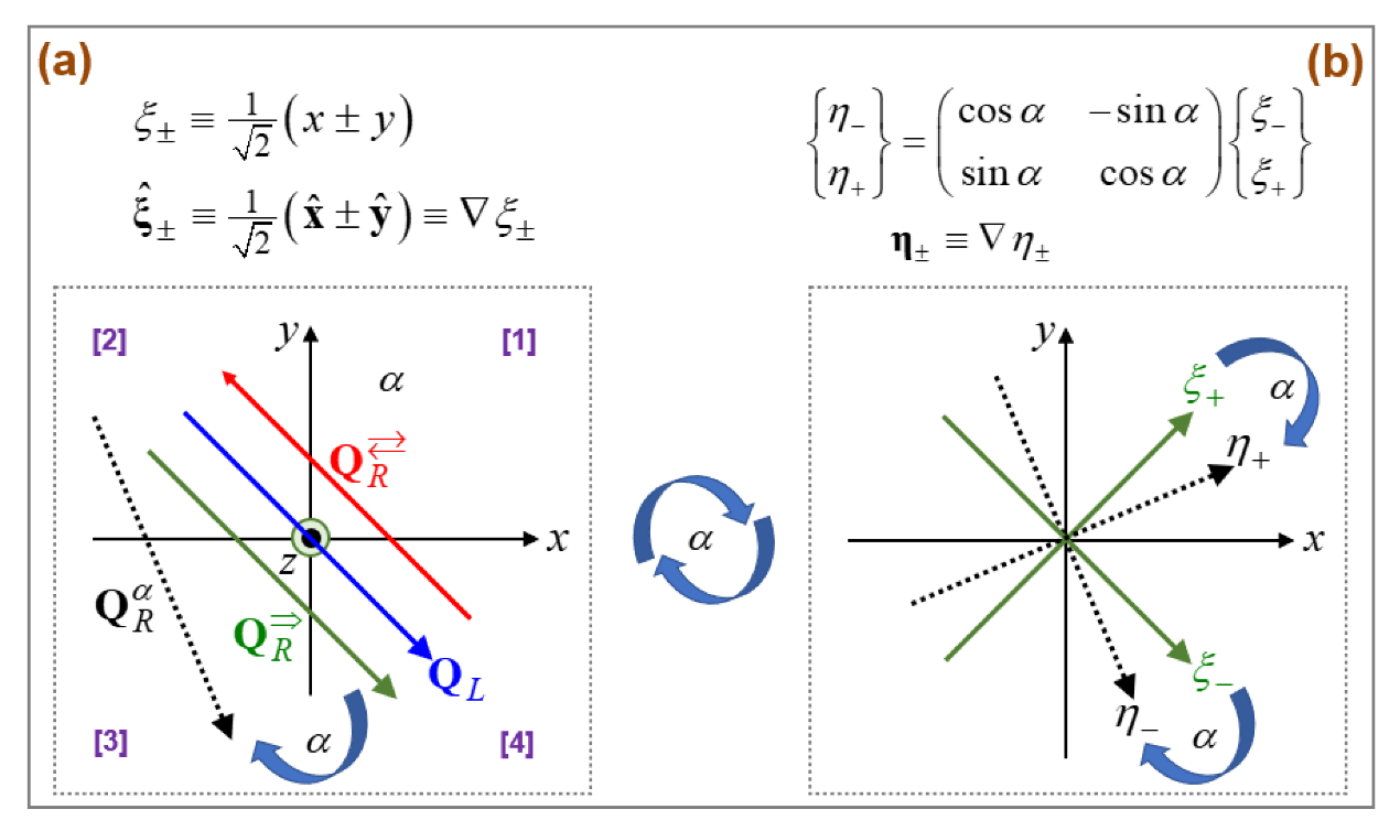
It is appropriate from the form $\exp \left[\pm i{k}_{LR}\frac{1}{\sqrt{2}}\left(x-y\right)\right]$ to introduce the following pair of characteristic coordinates ${\xi }_{\pm }\equiv \frac{1}{\sqrt{2}}\left(x\pm y\right)$ and their corresponding vectors ${\widehat{\xi }}_{\pm }\equiv \nabla {\xi }_{\pm }\equiv \frac{1}{\sqrt{2}}\left(\widehat{x}\pm \widehat{y}\right)$ [39]. We further define a pair of rotated (proper) characteristic coordinates ${\eta }_{\pm }$ and their corresponding vectors ${\eta }_{\pm }\equiv \nabla {\eta }_{\pm }$ [17]. Let us list below their definitions and attendant properties, while consulting Figure 1.

$$\begin{array}{l}\{\begin{array}{l}{\xi }_{\pm }\equiv \frac{1}{\sqrt{2}}\left(x\pm y\right)\\ {\widehat{\xi }}_{\pm }\equiv \frac{1}{\sqrt{2}}\left(\widehat{x}\pm \widehat{y}\right)\end{array},\begin{array}{c}\end{array}\left\{\begin{array}{c}{\eta }_{-}\\ {\eta }_{+}\end{array}\right\}=\left(\begin{array}{cc}\cos \alpha & -\sin \alpha \\ \sin \alpha & \cos \alpha \end{array}\right)\left\{\begin{array}{c}{\xi }_{-}\\ {\xi }_{+}\end{array}\right\}\begin{array}{c}\end{array}\Rightarrow \begin{array}{c}\end{array}\\ \{\begin{array}{l}{\eta }_{\pm }\equiv \frac{1}{\sqrt{2}}\left[\left(\cos \alpha \pm \sin \alpha \right)x\pm \left(\cos \alpha \mp \sin \alpha \right)y\right]\\ {\widehat{\eta }}_{\pm }\equiv \frac{1}{\sqrt{2}}\left[\left(\cos \alpha \pm \sin \alpha \right)\widehat{x}\pm \left(\cos \alpha \mp \sin \alpha \right)\widehat{y}\right]\end{array}\begin{array}{c}\end{array}\Rightarrow \begin{array}{c}\end{array}\\ \{\begin{array}{l}{\widehat{\xi }}_{\pm }\equiv \nabla {\xi }_{\pm },\begin{array}{c}\end{array}{\widehat{\xi }}_{\pm }\times \widehat{z}=\pm {\widehat{\xi }}_{\mp },\begin{array}{c}\end{array}\left|{\widehat{\xi }}_{\pm }\right|=1\\ {\widehat{\eta }}_{\pm }\equiv \nabla {\eta }_{\pm },\begin{array}{c}\end{array}{\widehat{\eta }}_{\pm }\times \widehat{z}=\pm {\widehat{\eta }}_{\mp },\begin{array}{c}\end{array}\left|{\widehat{\eta }}_{\pm }\right|=1\end{array},\begin{array}{c}\end{array}\{\begin{array}{l}{\widehat{\xi }}_{\pm }·{\eta }_{\pm }=\cos \alpha \\ {\widehat{\xi }}_{\pm }\times {\widehat{\eta }}_{\pm }=-\sin \alpha \widehat{z}\end{array}\end{array}$$

(16)

We learn that both of $\left\{{\widehat{\xi }}_{-},{\widehat{\xi }}_{+},\widehat{z}\right\}$ and $\left\{{\widehat{\eta }}_{-},{\widehat{\eta }}_{+},\widehat{z}\right\}$ are right handed triads of basis vectors as $\left\{\widehat{x},\widehat{y},\widehat{z}\right\}$, while $\widehat{z}$ is the common axial vector [10]. Take further notice that the rotation angle $\alpha \in ℝ$ is a specifiable constant in this study. In stark contrast, the usual azimuthal angle $\phi \in ℝ$ in both cylindrical and spherical polar coordinates is defined through $\tan \phi \equiv y/x$ [3]. Hence, $\phi$ is an independent parameter measured in the counter-clockwise direction on the $xy$-plane. Since $\alpha \ne \phi$, we introduced a different symbol of $\alpha$.

We can prove from Equation (16) the relationship ${\widehat{\xi }}_{\pm }·{\eta }_{\pm }=\cos \alpha$ of Equation (16), thus falling in conformance with the definition of the clockwise rotation angle $\alpha$. Both characteristic pairs $\left\{{\xi }_{\pm },{\eta }_{\pm }\right\}$ and their respective characteristic vectors $\left\{{\widehat{\xi }}_{\pm },{\widehat{\eta }}_{\pm }\right\}$ are straight lines on the physical $xy$-plane. Yet, the rotated pair $\left\{{\eta }_{\pm },{\widehat{\eta }}_{\pm }\right\}$ can be considered highly nonlinear in the clockwise rotation angle $\alpha$. Indeed, this nonlinear dependence will turn out to be a key player in the symmetry argument of this study.

With the help of Equation (16), the aforementioned solution $Q_{LR}$ found from Equation (15) can be specialized into the following three types of vectors $\left\{Q_L,Q_R^{\Rightarrow },Q_R^{\rightleftarrows }\right\}$ [28].

$$\{\begin{array}{l}{Q}_{LR}=Q_{LR}\frac{1}{\sqrt{2}}\left(\widehat{z}\mp {\widehat{\xi }}_{+}\right)\exp \left(\pm i{k}_{LC}{\xi }_{-}\right)\\ Q_{LR}\in \left\{\begin{array}{c}{Q}_L\\ Q_R\end{array}\right\}\end{array}\begin{array}{c}\end{array}\Rightarrow \begin{array}{c}\end{array}\{\begin{array}{l}{Q}_L=Q_L\frac{1}{\sqrt{2}}\left(\widehat{z}-i{\widehat{\xi }}_{+}\right)\exp \left(i{k}_L{\xi }_{-}\right)\\ Q_R:\begin{array}{c}\end{array}\{\begin{array}{l}{Q}_R^{\Rightarrow }=Q_R^{\Rightarrow }\frac{1}{\sqrt{2}}\left(\widehat{z}+i{\widehat{\xi }}_{+}\right)\exp \left(i{k}_R{\xi }_{-}\right)\\ Q_R^{\rightleftarrows }=Q_R^{\rightleftarrows }\frac{1}{\sqrt{2}}\left(\widehat{z}-i{\widehat{\xi }}_{+}\right)\exp \left(-i{k}_R{\xi }_{-}\right)\end{array}\end{array}$$

(17)

Here, we neglected the common temporal factor $e^{-it}$, which has been rendered dimensionless according to Equation (2). There is another solution $\frac{1}{\sqrt{2}}\left(\widehat{z}+{\widehat{\xi }}_{+}\right)\exp \left(-i{k}_L{\xi }_{-}\right)$ in addition to the left wave $Q_L=Q_L\frac{1}{\sqrt{2}}\left(\widehat{z}-i{\widehat{\xi }}_{+}\right)\exp \left(i{k}_L{\xi }_{-}\right)$ presented in the above set. To fix an idea, we selected only $Q_L$, which serves as a reference wave in this study. In stark contrast, the right wave $Q_R$ is specialized into two vectors $\left\{Q_R^{\Rightarrow },Q_R^{\rightleftarrows }\right\}$. In conventional sense, a linear combination of the co-propagating pair $\left\{Q_L,Q_R^{\Rightarrow }\right\}$ constitutes an elliptically polarized plane wave [21,22]. Moreover, there will be no standing waves as a result of the collision between $\left\{Q_L,Q_R^{\rightleftarrows }\right\}$ since $\left|k_L\right|\ne \left|k_R\right|$ for a chiral medium [10].

The vectors $\frac{1}{\sqrt{2}}\left(\widehat{z}\mp {\widehat{\xi }}_{+}\right)\exp \left(\pm i{k}_{LC}{\xi }_{-}\right)$ have a rotational character due to the vector $\widehat{z}\mp {\widehat{\xi }}_{+}$, while being advanced on the ${\xi }_{\pm }$-plane. Resultantly, these vectors could undergo either spiral or helical trajectories [2,3,9,11]. A non-zero field helicity is linked to the existence of the $z$-component in all $Q$’s listed in Equation (17) along the rotation axis [2]. Refractions through a planar slab offer an existence of co- and counter-propagating waves [25]. Since all vectors in Equation (17) carry spatially homogeneous polarizations, unlike in [9], the ensuing analysis in this study is rather straightforward.

Notice from Equation (4) that both of $\left\{k_L,k_R\right\}$ assume positive signs under the condition of a small (weak) chirality parameter such that either $\left|\beta \sqrt{\epsilon \mu }\right|<1$ or $\left|\kappa \right|<\sqrt{\epsilon \mu }$ [2,3,11,28]. Correspondingly, $k_L,k_R>0$ is assumed throughout this study. As displayed in Figure 1a, $Q_L$ then undergoes propagations from the second quadrant denoted by ‘[2]’ to the fourth quadrant denoted by ‘[4]’ on the $xy$-plane. Because the right wave $Q_R^{\Rightarrow }$ in Equation (17) carries its phase speed $k_R$ of the same sign as $k_L$ for $Q_L$, the pair $\left\{Q_L,Q_R^{\Rightarrow }\right\}$ constitutes a co-propagating pair.

In comparison, the pair $\left\{Q_L,Q_R^{\rightleftarrows }\right\}$ constitutes a counter-propagating pair, because the right wave $Q_R^{\rightleftarrows }$ in Equation (17) carries its phase speed $-k_R$ of the opposite sign to $k_L$ for $Q_L$. This is the reason why we have intentionally chosen the superscripts $\left\{\Rightarrow ,\rightleftarrows \right\}$ to denote such pairs of co- and counter-propagations. Any wary reader can easily verify the curl conditions that $\nabla \times Q_L=k_L{Q}_L$, $\nabla \times Q_R^{\Rightarrow }=-k_R{Q}_R^{\Rightarrow }$, and $\nabla \times Q_R^{\rightleftarrows }=-k_R{Q}_R^{\rightleftarrows }$ for Equation (17). Consulting Figure 1b, let us replace the space-fixed parameters $\left\{{\widehat{\xi }}_{+},{\xi }_{-}\right\}$ of $Q_R^{\Rightarrow }=Q_R^{\Rightarrow }\frac{1}{\sqrt{2}}\left(\widehat{z}+i{\widehat{\xi }}_{+}\right)\exp \left(i{k}_R{\xi }_{-}\right)$ in Equation (17) with their rotated parameters $\left\{{\widehat{\eta }}_{+},{\eta }_{-}\right\}$ to form another solution vector as follows.

$$\{\begin{array}{l}\left\{{\widehat{\xi }}_{+},{\xi }_{-}\right\}\\ Q_R^{\Rightarrow }=Q_R^{\Rightarrow }\frac{1}{\sqrt{2}}\left(\widehat{z}+i{\widehat{\xi }}_{+}\right)\exp \left(i{k}_R{\xi }_{-}\right)\end{array}\begin{array}{c}\end{array}\Rightarrow \begin{array}{c}\end{array}\{\begin{array}{l}\left\{{\widehat{\eta }}_{+},{\eta }_{-}\right\}\\ Q_R^{\alpha }=Q_R^{\alpha }\frac{1}{\sqrt{2}}\left(\widehat{z}+i{\widehat{\eta }}_{+}\right)\exp \left(i{k}_R{\eta }_{-}\right)\end{array}$$

(18)

Here, the superscript $\alpha$ signifies that $Q_R^{\alpha }$ is a right wave rotated clockwise through the angle $\alpha$ as measured from the right wave $Q_R^{\Rightarrow }$. It is obvious that this rotated vector $Q_R^{\alpha }$ satisfies all the necessary conditions listed in Equation (14), namely, $\nabla ·Q_R^{\alpha }=0$, $\nabla \times Q_R^{\alpha }=-k_R{Q}_R^{\alpha }$, and ${\nabla }^2{Q}_R^{\alpha }+k_R^2{Q}_R^{\alpha }=0$. In fact, $Q_R^{\alpha }$ of Equation (18) encompasses both $Q_R^{\Rightarrow }$ and $Q_R^{\rightleftarrows }$ of Equation (17) as two special cases. In other words, setting $\alpha =0$ in Equation (16) leads to ${\xi }_{\pm }={\eta }_{\pm }$ and ${\widehat{\xi }}_{\pm }={\widehat{\eta }}_{\pm }$ in Equation (15), thus leading to $Q_R^{\alpha }=Q_R^{\Rightarrow }$. Likewise, setting $\alpha =\pi$ in Equation (16) leads to ${\xi }_{\pm }=-{\eta }_{\pm }$ and ${\widehat{\xi }}_{\pm }=-{\widehat{\eta }}_{\pm }$ in Equation (15), thus leading to $Q_R^{\alpha }=Q_R^{\rightleftarrows }$. Consequently, the pair of $\left\{Q_L,Q_R^{\alpha }\right\}$ for $0<\alpha <\pi$ (two end angles being subtracted) designates a pair of obliquely colliding waves.

It is worth stressing that this kind of thorough discussion on $Q_R^{\alpha }$ presented in Equation (18) has been handled only by a few, for instance, [17]. Notwithstanding, only an achiral medium was considered by [17]. In comparison, $Q_R^{\alpha }$ has been discussed neither by [21] nor by [22]. Hence, our illumination parameters for the pair $\left\{Q_L,Q_R^{\alpha }\right\}$ are $\left\{{\xi }_{-},{\eta }_{-},\alpha ,Q_L,Q_R^{\alpha }\right\}$ [11]. We have thus accomplished a type of ‘switchable directional excitation’ [25].

Based further on the fields $\left\{E_{LR}^{\alpha },H_{LR}^{\alpha }\right\}$, let us customize the EM and reactive energy densities derived in Equation (6) as follows under the assumption $\epsilon \mu >0$.

$$\{\begin{array}{l}{I}_{LR}^{\alpha }\equiv \frac{1}{2}\left[\epsilon {\left(E_{LR}^{\alpha }\right)}^{*}·E_{LR}^{\alpha }+\mu {\left(H_{LR}^{\alpha }\right)}^{*}·H_{LR}^{\alpha }\right]=\sqrt{\epsilon \mu }\left(Z^{-1}{\left|Q_L\right|}^2+Z{\left|Q_R^{\alpha }\right|}^2\right)\\ J_{LR}^{\alpha }\equiv \frac{1}{2}\left[\epsilon {\left(E_{LR}^{\alpha }\right)}^{*}·E_{LR}^{\alpha }-\mu {\left(H_{LR}^{\alpha }\right)}^{*}·H_{LR}^{\alpha }\right]=0\end{array}$$

(19)

An alternative form $I_{LR}^{\alpha }=\epsilon {\left|Q_L\right|}^2+\mu {\left|Q_{LR}^{\alpha }\right|}^2$ is acceptable as well, where the factor of half (not the half arising from time averaging) happens to be missing. It is noticeable that the cross terms ${\left(Q_L\right)}^{*}·Q_R^{\alpha }$ and $Q_L·{\left(Q_R^{\alpha }\right)}^{*}$ cancel each other for $I_{LR}^{\alpha }$. Meanwhile, it surprises us that the resulting reactive energy density $J_{LR}^{\alpha }$ identically vanishes for any pair $\left\{\left|Q_L\right|,\left|Q_{LR}^{\alpha }\right|\right\}$ for any strengths of the two constituent waves whenever $\left\{Q_L,Q_{LR}^{\alpha }\right\}$ satisfy Equation (14).

Based on the fields $\left\{E_{LR}^{\alpha },H_{LR}^{\alpha }\right\}$ in terms of $\left\{Q_L,Q_R^{\alpha }\right\}$ according to Equation (13), we form both complex helicity $E_{LR}^{\alpha }·{\left(H_{LR}^{\alpha }\right)}^{*}$ and Poynting vectors $E_{LR}^{\alpha }\times {\left(H_{LR}^{\alpha }\right)}^{*}$ as follows [1].

$$\{\begin{array}{l}{E}_{LR}^{\alpha }·{\left(H_{LR}^{\alpha }\right)}^{*}=i\left(Z^{-1}{\left|Q_L\right|}^2-Z{\left|Q_R^{\alpha }\right|}^2\right)+2\mathrm{Re}\left[Q_R^{\alpha }·{\left(Q_L\right)}^{*}\right]\\ E_{LR}^{\alpha }\times {\left(H_{LR}^{\alpha }\right)}^{*}=i\left[Z^{-1}{Q}_L\times Q_L^{*}-Z{Q}_R^{\alpha }\times {\left(Q_R^{\alpha }\right)}^{*}\right]+2i\mathrm{Im}\left[Q_R^{\alpha }\times {\left(Q_L\right)}^{*}\right]\end{array}$$

(20)

By taking real and imaginary parts of Equation (20) according to Equation (7), we arrive at the following two pairs of EM and reactive parameters after finding the intermediaries of $E_{LR}^{\alpha }·{\left(H_{LR}^{\alpha }\right)}^{*}$ and $E_{LR}^{\alpha }\times {\left(H_{LR}^{\alpha }\right)}^{*}$.

$$\begin{array}{l}\{\begin{array}{l}{C}_{LR}^{\alpha }=Z^{-1}{\left|Q_L\right|}^2-Z{\left|Q_R^{\alpha }\right|}^2\\ K_{LR}^{\alpha }=2\mathrm{Re}\left[{\left(Q_L\right)}^{*}·Q_R^{\alpha }\right]\end{array}\\ \{\begin{array}{l}{P}_{LR}^{\alpha }=\mathrm{Im}\left[Z{Q}_R^{\alpha }\times {\left(Q_R^{\alpha }\right)}^{*}-Z^{-1}{Q}_L\times {\left(Q_L\right)}^{*}\right]\\ R_{LR}^{\alpha }=\mathrm{Re}\left[Z^{-1}{Q}_L\times {\left(Q_L\right)}^{*}-Z{Q}_R^{\alpha }\times {\left(Q_R^{\alpha }\right)}^{*}\right]-2\mathrm{Im}\left[{\left(Q_L\right)}^{*}\times Q_R^{\alpha }\right]\end{array}\end{array}$$

(21)

We learn from Equation (21) that both $\left\{C_{LR}^{\alpha },P_{LR}^{\alpha }\right\}$ involve self-products between the two constituent waves, whereas both $\left\{K_{LR}^{\alpha },R_{LR}^{\alpha }\right\}$ incur cross-products. An exception is that $R_{LR}^{\alpha }$ carries self-products as well. It turns out sometimes that $K_{LR}^{\alpha }=2\mathrm{Re}\left[{\left(Q_L\right)}^{*}·Q_R^{\alpha }\right]$ carries a more physical importance because of its interference implications than $C_{LR}^{\alpha }=Z^{-1}{\left|Q_L\right|}^2-Z{\left|Q_R^{\alpha }\right|}^2$ that bears only a magnitude information [7,12].

Consider the polarization states of $\left\{Q_L,Q_R^{\alpha }\right\}$ in the circular $Q$-space: ${\left|Q_L\right|}^{-2}\mathrm{Im}\left[{\left(Q_L\right)}^{*}\times Q_L\right]={\widehat{\xi }}_{-}$ and ${\left|Q_R^{\alpha }\right|}^{-2}\mathrm{Im}\left[{\left(Q_R^{\alpha }\right)}^{*}\times Q_R^{\alpha }\right]=-{\widehat{\eta }}_{-}$ for a left wave and an oblique right wave, respectively [25]. Therefore, the angle of polarization rotation is equal to $-\alpha$, thereby being the negative of the oblique collision angle according to ${\widehat{\xi }}_{\pm }·{\eta }_{\pm }=\cos \alpha$ in Equation (16). The phase modulation is thus achieved by $\alpha$ in our study. With the help of Equations (12) and (13), we specialize the spin AM density $M\equiv \frac{1}{2}\mathrm{Im}\left(\epsilon E^{*}\times E+\mu H^{*}\times H\right)$ to our obliquely colliding waves as follows.

$$\begin{array}{l}{M}_{LR}^{\alpha }\equiv \frac{1}{2}\mathrm{Im}\left[\epsilon {\left(E_{LR}^{\alpha }\right)}^{*}\times E_{LR}^{\alpha }+\mu {\left(H_{LR}^{\alpha }\right)}^{*}\times H_{LR}^{\alpha }\right]\\ \begin{array}{c}\begin{array}{c}\end{array}=\epsilon \mathrm{Im}\left[{\left(Q_L\right)}^{*}\times Q_L\right]+\end{array}\mu \mathrm{Im}\left[{\left(Q_R^{\alpha }\right)}^{*}\times Q_R^{\alpha }\right]+Z\left(\mu -\epsilon \right)\mathrm{Re}\left[{\left(Q_L\right)}^{*}\times Q_R^{\alpha }\right]\end{array}$$

(22)

Here, we assumed $\epsilon ,\mu \in ℝ$. Resultantly, the average spin AM density $M_{LR}^{\alpha }$ takes a mixture of symmetric and anti-symmetric forms with respect to $\left\{\epsilon ,\mu \right\}$. It turns out that both parts $\left\{\mathrm{Re}\left[{\left(Q_L\right)}^{*}\times Q_R^{\alpha }\right],\mathrm{Im}\left[{\left(Q_L\right)}^{*}\times Q_R^{\alpha }\right]\right\}$ contain not only the longitudinal vector ${\widehat{\xi }}_{-}-{\widehat{\eta }}_{-}$ but also the transverse vector $\widehat{z}$ [1,20,29]. The 3D polarization vector is thus given by $M_{LR}^{\alpha }/I_{LR}^{\alpha }$, being normalized by the average energy density $I_{LR}^{\alpha }$ provided by Equation (19).

It is stressed that Equations (19)–(22) hold true for both types of constitutive relations presented in Equation (3). Utilizing Equations (17) and (18), various self- and cross-products between $\left\{Q_L,Q_R^{\alpha }\right\}$ necessary for Equation (21) are straightforwardly evaluated in Supplementary Material. Those formulas are made concise by introducing the following pair $\left\{{\Gamma }_{LR}^{\alpha },{\delta }_{LR}^{\alpha }\right\}$ of parameters.

$$\{\begin{array}{l}{\Gamma }_{LR}^{\alpha }\equiv k_L{\xi }_{-}-k_R{\eta }_{-}\\ {\left(Q_L\right)}^{*}{Q}_R^{\alpha }\equiv \left|{\left(Q_L\right)}^{*}{Q}_R^{\alpha }\right|\exp \left(-i{\delta }_{LR}^{\alpha }\right)\end{array}$$

(23)

Here, we have made use of both $\left\{k_L,k_R\right\}$ of Equation (4) and $\left\{{\xi }_{-}{\eta }_{-}\right\}$ of Equation (16). Firstly, we defined an ‘interference function’ ${\Gamma }_{LR}^{\alpha }\left(\alpha \right)$ that depends especially on the oblique angle $\alpha$, thus signifying interactions between the reference left wave and an oblique right wave [11,33]. The magnitude $\left|{\xi }_{-}-{\eta }_{-}\right|$ is an offset distance [25]. Secondly, we introduced a specifiable ‘amplitude factor’ ${\delta }_{LR}^{\alpha }$ for a given pair $\left\{Q_L,Q_R^{\alpha }\right\}$ of specified magnitudes [6]. For concreteness, we set $0\le {\delta }_{LR}^{\alpha }<2\pi$. It is further noted that $\left|{\left(Q_L\right)}^{*}{Q}_R^{\alpha }\right|\ne \left|Q_L\right|\left|Q_R^{\alpha }\right|$ in general. This interference function ${\Gamma }_{LR}^{\alpha }\left(\epsilon ,\mu ,\alpha ,x,y;\beta \right)$ or ${\Gamma }_{LR}^{\alpha }\left(\epsilon ,\mu ,\alpha ,x,y;\kappa \right)$ introduced in Equation (23) is the first key parameter for a two-wave system, whereas the amplitude factor ${\delta }_{LR}^{\alpha }$ defined by Equation (23) is the second key parameter [1,4,17].

We further evaluate the as-yet-undetermined three parameters $\left\{K_{LR}^{\alpha },P_{LR}^{\alpha },R_{LR}^{\alpha },M_{LR}^{\alpha }\right\}$ presented in Equations (21) and (22) by use of Equation (23) and necessary dot- and cross-products evaluated in Supplementary Material.

$$\begin{array}{l}{K}_{LR}^{\alpha }=\left(1-\cos \alpha \right)\left|{\left(Q_L\right)}^{*}{Q}_R^{\alpha }\right|\cos \left({\Gamma }_{LR}^{\alpha }+{\delta }_{LR}^{\alpha }\right)\\ \{\begin{array}{l}{P}_{LR}^{\alpha }=Z^{-1}{\left|Q_L\right|}^2{\widehat{\xi }}_{-}+Z{\left|Q_R^{\alpha }\right|}^2{\eta }_{-}\\ R_{LR}^{\alpha }=-\sqrt{2}\left|{\left(Q_L\right)}^{*}{Q}_R^{\alpha }\right|\cos \left({\Gamma }_{LR}^{\alpha }+{\delta }_{LR}^{\alpha }\right)\frac{1}{\sqrt{2}}\left({\widehat{\xi }}_{-}-{\eta }_{-}\right)\end{array}\\ M_{LR}^{\alpha }=\epsilon {\left|Q_L\right|}^2{\widehat{\xi }}_{-}-\mu {\left|Q_R^{\alpha }\right|}^2{\widehat{\eta }}_{-}\\ \begin{array}{c}\end{array}+Z\left(\mu -\epsilon \right)\left|{\left(Q_L\right)}^{*}{Q}_R^{\alpha }\right|\frac{1}{2}\left[\sin \alpha \cos \left({\Gamma }_{LR}^{\alpha }+{\delta }_{LR}^{\alpha }\right)\widehat{z}+\sin \left({\Gamma }_{LR}^{\alpha }+{\delta }_{LR}^{\alpha }\right)\left({\widehat{\xi }}_{-}-{\widehat{\eta }}_{-}\right)\right]\end{array}$$

(24)

The two leading components $\epsilon {\left|Q_L\right|}^2{\widehat{\xi }}_{-}-\mu {\left|Q_R^{\alpha }\right|}^2{\widehat{\eta }}_{-}$ of $M_{LR}^{\alpha }$ are not dependent on the interference function ${\Gamma }_{LR}^{\alpha }$. As stated shortly before as regards Equation (22), the remaining components $\left\{\widehat{z},{\widehat{\xi }}_{-}-{\widehat{\eta }}_{-}\right\}$ of $M_{LR}^{\alpha }$ are in-phase and out-of-phase with respect to $\left\{K_{LR}^{\alpha },R_{LR}^{\alpha }\right\}$. Their common multiplier $\left(\mu -\epsilon \right)$ appearing on the interference term $\mathrm{Re}\left[{\left(Q_L\right)}^{*}\times Q_R^{\alpha }\right]$ in Equation (22) and in Equation (24) prompts us to examine the following relation [6,25].

$$Z^{-1}-Z\equiv \sqrt{\frac{\epsilon }{\mu }}-\sqrt{\frac{\mu }{\epsilon }}=\frac{\epsilon -\mu }{\sqrt{\epsilon \mu }}$$

(25)

Notice incidentally that the numerator $\epsilon -\mu$ on the right-hand side of Equation (25) is related to the second matrix for a rate of shearing on the right-hand side of Equation (9). As an example of Equation (25), $\mu =p\left(\epsilon -1\right)+1$ with the duality parameter $p$ over $0\le p\le 1$ has been employed in [7] so that $\epsilon -\mu =\left(\epsilon -1\right)\left(1-p\right)$. In this case, it is found that ${\left[\left(d/dp\right)\left(Z^{-1}-Z\right)\right]|}_{\epsilon }>0$.

Let us find the two limits of the pair $\left\{{\eta }_{-}^{\alpha },{\Gamma }_{LR}^{\alpha }\right\}$ from Equations (16) and (23) as follows [17].

$$\alpha =0:\begin{array}{c}\end{array}\{\begin{array}{l}{\eta }_{-}^{\alpha =0}=\frac{1}{\sqrt{2}}\left(x-y\right)={\xi }_{-}\\ {\Gamma }_{LR}^{\alpha =0}=0\end{array},\begin{array}{c}\end{array}\alpha =\pi :\begin{array}{c}\end{array}\{\begin{array}{l}{\eta }_{-}^{\alpha =\pi }=-\frac{1}{\sqrt{2}}\left(x-y\right)=-{\xi }_{-}\\ {\Gamma }_{LR}^{\alpha =\pi }=\left(k_L+k_R\right){\xi }_{-}\end{array}$$

(26)

We then find the two limits for the key bilinear parameters of a co-propagating case and a counter-propagating case, respectively, from Equations (23) and (24) [10].

$$\begin{array}{l}\alpha =0:\begin{array}{c}\end{array}{K}_{LR}^{\alpha =0}=0,\begin{array}{c}\end{array}{P}_{LR}^{\alpha =0}={\left(\epsilon \mu \right)}^{-1/2}{I}_{LR}^{\alpha }{\widehat{\xi }}_{-},\begin{array}{c}\end{array}{R}_{LR}^{\alpha =0}=0\\ \alpha =\pi :\begin{array}{c}\end{array}\{\begin{array}{l}{K}_{LR}^{\alpha =\pi }=2\left|{\left(Q_L\right)}^{*}{Q}_R^{\rightleftarrows }\right|\cos \left[\left(k_L+k_R\right){\xi }_{-}+{\delta }_{LR}^{\alpha }\right]\\ P_{LR}^{\alpha =\pi }=C_{LR}^{\alpha }{\widehat{\xi }}_{-}\\ R_{LR}^{\alpha =\pi }=-2\left|{\left(Q_L\right)}^{*}{Q}_R^{\rightleftarrows }\right|\cos \left[\left(k_L+k_R\right){\xi }_{-}+{\delta }_{LR}^{\alpha }\right]{\widehat{\xi }}_{-}=-K_{LR}^{\alpha =\pi }{\widehat{\xi }}_{-}\end{array}\end{array}$$

(27)

With the limits in Equation (26), $M_{LR}^{\alpha =0}$ and $M_{LR}^{\alpha =\pi }$ can be easily deduced from Equation (24). As seen from Supplementary Material, ${\left(Q_L\right)}^{*}·Q_R^{\alpha }=\left|{\left(Q_L\right)}^{*}{Q}_R^{\alpha }\right|\frac{1}{2}\left(1-\cos \alpha \right)\exp \left[-i\left({\Gamma }_{LR}^{\alpha }+{\delta }_{LR}^{\alpha }\right)\right]$ so that $\left\{Q_L,Q_R^{\alpha }\right\}$ are of crossed polarizations with each other at $\alpha =0$ if viewed in the circular $Q$-space.

As a direct consequence of this pair of limit behaviors in Equation (26), the pair of $\left\{Q_L,Q_R^{\alpha }\right\}$ for $0<\alpha <\pi$ (two end angles being subtracted) designates a spatially non-uniform wave [3,8]. Based on $\left\{Q_L,Q_R^{\alpha }\right\}$ and the transformation rule in Equation (13), let us form a pair of electric and magnetic fields $\left\{E_{LR}^{\alpha },H_{LR}^{\alpha }\right\}$ for such a combined wave by $E_{LR}^{\alpha }=Q_L-iZ{Q}_R^{\alpha }$ and $H_{LR}^{\alpha }=-i{Z}^{-1}{Q}_L+Q_R^{\alpha }$ [21,22]. Because $\left\{E_{LR}^{\alpha },H_{LR}^{\alpha }\right\}$ are described by two independent spatial coordinates, namely, $\left\{{\xi }_{-},{\eta }_{-}\right\}$, the pair $\left\{Q_L,Q_R^{\alpha }\right\}$ exhibits a non-uniform $X$-wave-like configuration on the circular $Q$-space [29,36].

4. Symmetry with Respect to Medium Chirality

We recognize from Equations (26) and (27) the importance of the algebraic average $\frac{1}{2}\left(k_R+k_L\right)$ appearing for the counter-propagating pair $\left\{Q_L,Q_R^{\rightleftarrows }\right\}$ in Equation (17), the latter being evaluated with $\alpha =\pi$. It is curious enough that $\sqrt{\epsilon \mu }$ is the inverse of the geometric mean between $\left\{k_L,k_R\right\}$ as seen from Equation (4) for the curl-$\beta$-based constitutive relations. From Equation (4), this algebraic average $\frac{1}{2}\left(k_R+k_L\right)$ takes the following simple forms [27].

$$\{\begin{array}{l}{C}_{\beta }^{curl}:\begin{array}{c}\end{array}\frac{1}{2}\left(k_R+k_L\right)=\frac{\sqrt{\epsilon \mu }}{1-{\beta }^2\epsilon \mu }\\ C_{\kappa }^{field}:\begin{array}{c}\end{array}\frac{1}{2}\left(k_R+k_L\right)=\sqrt{\epsilon \mu }\end{array}$$

(28)

Therefore, $\frac{1}{2}\left(k_R+k_L\right)$ is symmetric with respect to $\beta =0$ for $C_{\beta }^{field}$. In comparison, $\frac{1}{2}\left(k_R+k_L\right)$ is independent of $\kappa$ for $C_{\kappa }^{field}$, which can also be considered to signify symmetry with respect to $\kappa =0$. In this connection, let us revisit Equation (12) for the conservation law involving $\nabla ·M$. We notice in $\nabla ·M+{\left(1-\epsilon \mu {\beta }^2\right)}^{-1}2\epsilon \mu K=0$ for the curl-$\beta$-based constitutive relations $C_{\beta }^{field}$ can rewritten as $\nabla ·M+2k_L{k}_{R}K=0$ via Equation (4), which also features an evenness with respect to $\beta$. In stark contrast, it surprises us that $\nabla ·M=0$ does not explicitly contain $K$ (thus meaning an apparent independence on $\kappa$) for a chiral media with the field-$\kappa$-based constitutive relations $C_{\kappa }^{field}$.

Physically, both chirality parameters $\left\{\beta ,\kappa \right\}$ in Equation (3) are small. To find a relationship holding between $\left\{\beta ,\kappa \right\}$ in the limit $\beta ,\kappa \to 0$, consider temporarily the approximate version of Maxwell equations $\nabla \times E=i\mu H$ and $\nabla \times H=-i\epsilon E$ from Equations (3) and (5) for an achiral medium. Meanwhile, the constitutive relations $C_{\beta }^{field}$ in Equation (3) are reduced in the following fashion.

$$\beta \to 0:\begin{array}{c}\end{array}\{\begin{array}{l}\nabla \times E=i\mu H\\ \nabla \times H=-i\epsilon E\end{array}\begin{array}{c}\end{array}\Rightarrow \begin{array}{c}\end{array}{C}_{\beta }^{curl}:\begin{array}{c}\end{array}\{\begin{array}{l}D=\epsilon E+i\beta \epsilon \mu H\\ B=\mu H-i\beta \epsilon \mu E\end{array}$$

(29)

When comparing the reduced constitutive relations in Equation (29) with those for $C_{\kappa }^{field}$ defied in Equation (3), we find that $\kappa \to \beta \epsilon \mu$ as $\beta ,\kappa \to 0$ [21]. Of course, we are dealing with small chiral parameter with $\left|\beta \sqrt{\epsilon \mu }\right|<<1$ for $C_{\beta }^{curl}$ in Equation (4) such that both $\left\{k_L,k_R\right\}$ are positive as seen in Equation (4).

Let us come to the interference function ${\Gamma }_{LR}^{\alpha }\equiv k_L{\xi }_{-}-k_R{\eta }_{-}$ given in Equation (23). We find in Equation (8) that each of $\left\{k_L,k_R\right\}$ is odd in $\beta$ over $0<\alpha <\pi$ with the attendant anti-symmetry that $k_L\left(\pm \beta \right)=k_R\left(\mp \beta \right)$ with $\sqrt{\epsilon \mu }$ fixed. Consequently, for a pair of obliquely colliding waves, ${\Gamma }_{LR}^{\alpha }\left(\beta \right)$ encompasses both odd and even features in $\beta$. In this connection, a key result of our study is identifying the transition with increasing $\alpha$ from asymmetry (anti-symmetry included) into symmetry as $\alpha \uparrow \pi$ as indicated by Equations (26) and (27). As seen on Equation (27) in case of counter-propagating waves with $\alpha =\pi$, we encounter an appearance of the collaborative factor $\left(k_L+k_R\right)$ within the cosine function $\cos \left[\left(k_L+k_R\right){\xi }_{-}+{\delta }_{LR}^{\alpha }\right]$ [9]. Indeed, the symmetry exhibited by a pair of counter-propagating waves is a rare event. This rarity can be imagined by the experimental fact that a slightest misalignment or an off-axis illumination between two presumably counter-propagating waves leads just to an obliquely colliding wave [25,28].

Let us hence numerically evaluate $\cos \left({\Gamma }_{LR}^{\alpha }+{\delta }_{LR}^{\alpha }\right)$ in Equation (24) with ${\Gamma }_{LR}^{\alpha }\equiv k_L{\xi }_{-}-k_R{\eta }_{-}$ in Equation (23) for a pair of obliquely colliding waves. The optical properties are set such that $\epsilon \mu =4$, while the amplitude factor ${\delta }_{LR}^{\alpha }$ in Equation (23) is set to zero for simplicity. For the pair $\left\{x,y\right\}$, we took $x-y=1$ so that ${\xi }_{-}\equiv \frac{1}{\sqrt{2}}\left(x-y\right)=\frac{1}{\sqrt{2}}$ is fixed. In comparison, ${\xi }_{-}\equiv \frac{1}{\sqrt{2}}\left[\left(\cos \alpha -\sin \alpha \right)x-\left(\cos \alpha +\sin \alpha \right)y\right]$ in Equation (23) undergoes variations with varying $\alpha$. 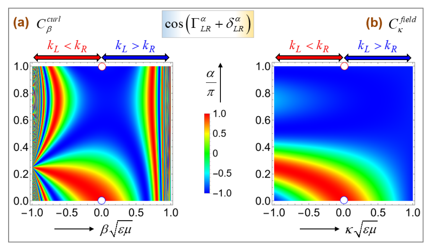Hence, we need to additionally specify $y$, which is set at $y=0$ in Figure 2.

Figure 2 shows ${\Gamma }_{LR}^{\alpha }\left(\epsilon ,\mu ,\alpha ,x,y;\beta \right)$ on panel (a) and ${\Gamma }_{LR}^{\alpha }\left(\epsilon ,\mu ,\alpha ,x,y;\kappa \right)$ on panel (b), based on the curl-$\beta$-based constitutive relations $C_{\beta }^{curl}$ and the field-$\kappa$-based constitutive relations $C_{\kappa }^{field}$, respectively, given in Equation (3). The vertical axis is taken to be the normalized rotation angle $\alpha /\pi$ over the range $0\le \alpha /\pi \le 1$. Meanwhile, the horizontal axis is chosen to be the normalized chirality parameters over the respective ranges of $-1\le \beta \sqrt{\epsilon \mu },\kappa \sqrt{\epsilon \mu }\le 1$. With $\epsilon \mu =4$ fixed, $-\frac{1}{2}<\beta <\frac{1}{2}$ and $-\frac{1}{2}<\kappa <\frac{1}{2}$ are hence implied on the respective panels. Such horizontal ranges ensure that $k_L,k_R\ge 0$ according to Equation (4). We placed two double-head arrows on top of each panel to show the zones with $k_L<k_R$ (in red) and $k_L>k_R$ (in blue), respectively.

To check the validity of numerical values, we evaluated ${\Gamma }_{LR}^{\alpha }$ on two special points on each of two panels of Figure 2. Both points are marked by circles in white fillings, while being evaluated for vanishing optical chirality, namely, $\beta =\kappa =0$. Therefore, Equation (4) gives rise to $k_R=k_L=\sqrt{\epsilon \mu }=2$ at both points lying on the central vertical lines. The doubling from $k_L$ to $k_R+k_L$ appearing in ${\Gamma }_{LR}^{\alpha =\pi }=\left(k_L+k_R\right){\xi }_{-}$ of Equation (26) is linked to the well-established fact that a typical standing wave is created by two counter-propagating waves, where the period of the intensity peaks is generally half the common wavelength [25,36]. The lower points in blue boundaries refer to $\alpha =0$ in correspondence to Equations (26) and (27), whereas the upper points in red boundaries refer to $\alpha =\pi$. Therefore, ${\Gamma }_{LR}^{\alpha }$ in Equation (26) is further evaluated as follows with the data $\epsilon \mu =4$, ${\delta }_{LR}^{\alpha }=0$, and $\left\{x,y\right\}=\left\{1,0\right\}$.

$$\begin{array}{l}\{\begin{array}{l}\alpha =0:\begin{array}{c}\end{array}{\Gamma }_{LR}^{\alpha =0}=\left(2\right)\frac{1}{\sqrt{2}}\left(1\right)-\left(2\right)\frac{1}{\sqrt{2}}\left[\left(1-0\right)1-\left(1+0\right)0\right]=0\\ \alpha =\pi :\begin{array}{c}\end{array}{\Gamma }_{LR}^{\alpha =\pi }=\left(2\right)\frac{1}{\sqrt{2}}\left(1\right)-\left(2\right)\frac{1}{\sqrt{2}}\left[\left(-1-0\right)1-\left(-1+0\right)0\right]=2\sqrt{2}\end{array}\\ \begin{array}{c}\end{array}\Rightarrow \begin{array}{c}\end{array}\{\begin{array}{l}\alpha =0:\begin{array}{c}\end{array}\cos \left({\Gamma }_{LR}^{\alpha =0}\right)=1\\ \alpha =\pi :\begin{array}{c}\end{array}\cos \left({\Gamma }_{LR}^{\alpha =\pi }\right)=\cos \left(2\sqrt{2}\right)\approx -0.951\end{array}\end{array}$$

(30)

According to the color bar lying on the center of Figure 2, the numerical values of the above pair of ${\Gamma }_{LR}^{\alpha }$ is thus confirmed. Otherwise, $\cos \left({\Gamma }_{LR}^{\alpha }\right)$ is seen to take varied values on the planes of $\left\{\alpha /\pi ,\beta \sqrt{\epsilon \mu }\right\}$ and $\left\{\alpha /\pi ,\kappa \sqrt{\epsilon \mu }\right\}$, respectively. Notice incidentally from Equation (23) that specifying the amplitude factor ${\delta }_{LR}^{\alpha }$ differently in $\cos \left({\Gamma }_{LR}^{\alpha }+{\delta }_{LR}^{\alpha }\right)$ could lead to $\cos \left({\Gamma }_{LR}^{\alpha }+{\delta }_{LR}^{\alpha }\right)=-1$ at $\alpha =\pi$ other than $\cos \left({\Gamma }_{LR}^{\alpha }\right)\approx -0.951$ given in Equation (30). By this way, phase control can be exercised to achieve a desired performance [25]. Both panels of Figure 2 being taken together, $\cos \left({\Gamma }_{LR}^{\alpha }\right)$ is not symmetric with respect to the vanishing chirality parameter at any $\alpha$ other than $\alpha =\pi$. Only at $\alpha =\pi$ designating a counter-propagating collision, does $\cos \left({\Gamma }_{LR}^{\alpha }\right)$ assume a symmetric feature.

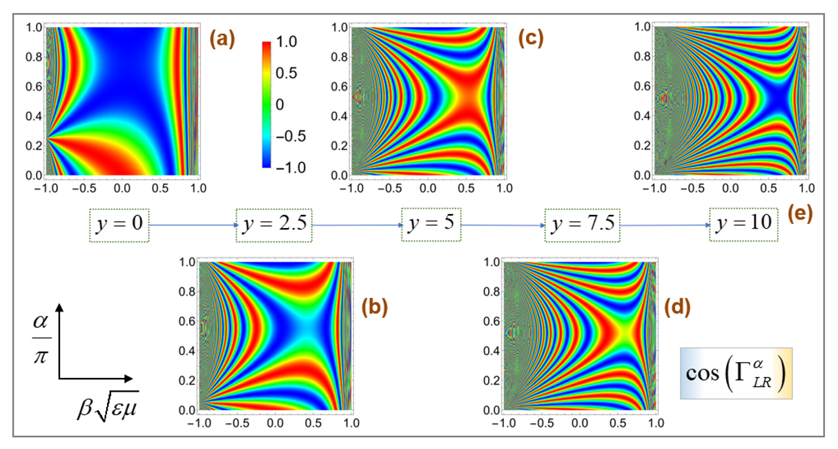
In correspondence to Figure 2a, we have made variations in $y$ for $\cos \left({\Gamma }_{LR}^{\alpha }\right)$ over $y=0,\frac{5}{2},\frac{10}{2},\frac{15}{2},\frac{20}{2}$ on five panels in Figure 3. All other parameters stay the same including $\sqrt{2}{\xi }_{-}\equiv x-y=1$. Therefore, the five panels are made with increasing field points from left to right such that $\left\{x,y\right\}=\left\{1,0\right\},\left\{\frac{7}{2},\frac{5}{2}\right\},\left\{\frac{12}{2},\frac{10}{2}\right\},\left\{\frac{17}{2},\frac{15}{2}\right\},\left\{\frac{22}{2},\frac{20}{2}\right\}$. Figure 3a is hence a reproduction of Figure 2a. The color bar located on the right of Figure 3a is applicable equally well to all panels of Figure 3.

Resultantly, the two invariant aspects of $\cos \left({\Gamma }_{LR}^{\alpha =0}\right)=1$ and $\cos \left({\Gamma }_{LR}^{\alpha =\pi }\right)\approx -0.951$ are still visible at $\beta =0$ on all panels of Figure 3. Of course, $\cos \left({\Gamma }_{LR}^{\alpha =\pi }\right)$ carries symmetry with respect to a vanishing medium chirality $\beta$. In addition, we confirm that the spatial variations on each panel are intensified as the field point is removed from the origin from panel (a) to panel (e). That is, the far-field effect manifests itself through higher spatial oscillations. We also find that the state $\cos \left({\Gamma }_{LR}^{\alpha =\pi }\right)$ is a fixed-point state for any combination of $\left\{x,y\right\}=\left\{y+1,y\right\}$ such that $\sqrt{2}{\xi }_{-}\equiv x-y=1$. Although an analogous set of five panels has been generated for Figure 2b for the other type of constitutive relations, it is not presented in this study for space reasons.

Movie 1 is a more continuous version of $\cos \left({\Gamma }_{LR}^{\alpha }\right)$ shown in Figure 3 for the curl-$\beta$-based constitutive relations $C_{\beta }^{curl}$, where one hundred panels are presented in sequel with an equal step of $\Delta y=\frac{1}{10}$ over the whole range $0\le y\le 10$. Likewise, Movie 2 is a more continuous version of $\cos \left({\Gamma }_{LR}^{\alpha }\right)$ corresponding to Figure 2b for the field-$\kappa$-based constitutive relations. The cancellations become stronger in the far field as seen in Figure 3e, whence the reactive properties carrying the factor $\cos \left({\Gamma }_{LR}^{\alpha }+{\delta }_{LR}^{\alpha }\right)$ become dominant in the near field as seen in Figure 3a [12,29,36,37]. See both $\left\{K_{LR}^{\alpha },R_{LR}^{\alpha }\right\}$ in Equation (24), where the interference function $\cos \left({\Gamma }_{LR}^{\alpha }+{\delta }_{LR}^{\alpha }\right)$ is incorporated.

5. Other Bilinear Parameters

With sufficient information on the interference function $\cos \left({\Gamma }_{LR}^{\alpha }+{\delta }_{LR}^{\alpha }\right)$ available so far, let us come back to the generic solutions: $\left\{I_{LR}^{\alpha },J_{LR}^{\alpha }\right\}$ in Equation (19), $C_{LR}^{\alpha }$ in Equation (21), and $\left\{K_{LR}^{\alpha },P_{LR}^{\alpha },R_{LR}^{\alpha },M_{LR}^{\alpha }\right\}$ in Equation (24) for more interpretation. Their special values in Equation (27) will be also examined. The fact is that $J_{LR}^{\alpha }=0$ in Equation (19) is only specific to our pair of obliquely colliding waves [37]. We have made a simple calculation of the reactive energy density for the EM fields resulting from the Mie scattering [22], which is not presented in this study. Resultantly, we learned that the reactive energy density is strongly non-zero, especially in the near field.

Recall the transformation rule in Equation (13) that there are two distinct representations of solutions: (i) the pair $\left\{Q_L,Q_R\right\}$ in the circular $Q$-space, and (ii) the pair $\left\{E,H\right\}$ in the physical $EH$-space. In this connection, Equation (19) offers two forms for the EM energy density. Namely, $I_{LR}^{\alpha }\equiv \frac{1}{2}\left[\epsilon {\left(E_{LR}^{\alpha }\right)}^{*}·E_{LR}^{\alpha }+\mu {\left(H_{LR}^{\alpha }\right)}^{*}·H_{LR}^{\alpha }\right]$ is the energy density in the physical $EH$-space, whereas $I_{LR}^{\alpha }=\sqrt{\epsilon \mu }\left(Z^{-1}{\left|Q_L\right|}^2+Z{\left|Q_R^{\alpha }\right|}^2\right)$ is its counterpart in the circular $Q$-space.

Meanwhile, we can consider the environ to be the medium through which both waves undergo propagations. The environmental effects show themselves up through the admittance $Z^{-1}\equiv \sqrt{\epsilon /\mu }$ and the impedance $Z\equiv \sqrt{\mu /\epsilon }$ differently for the left and oblique right waves [25]. Moreover, the environmental effects are log-anti-symmetric with the factors of $\left\{Z^{-1},Z\right\}$, respectively, as regards $I_{LR}^{\alpha }=\sqrt{\epsilon \mu }\left(Z^{-1}{\left|Q_L\right|}^2+Z{\left|Q_R^{\alpha }\right|}^2\right)$ in Equation (19). See the off-diagonal part of matrix $A$ in Equation (13). That is, the environ affects the EM energy density by a pair of logarithmic weightings, which are then modified equally by the additional factor of $\sqrt{\epsilon \mu }$.

Let us turn to Equation (21) listing the EM helicity $C_{LR}^{\alpha }=Z^{-1}{\left|Q_L\right|}^2-Z{\left|Q_R^{\alpha }\right|}^2$, which takes the form of square-norm difference [28]. From the energy viewpoint, $C_{LR}^{\alpha }$ signifies a difference between the environ-modified energy densities in the circular $Q$-space. The EM helicity is annihilated, namely, $C_{LR}^{\alpha }=0$, when $Z^{-1}{\left|Q_L\right|}^2=Z{\left|Q_R^{\alpha }\right|}^2$ [7]. Notice that the reactive energy density vanishes as $J_{LR}^{\alpha }=0$ in Equation (19) so that this pair $\left\{I_{LR}^{\alpha },J_{LR}^{\alpha }\right\}$ loses its usefulness. Instead, we have a complementary pair $\left\{{\left(\epsilon \mu \right)}^{-1/2}{I}_{LR}^{\alpha },C_{LR}^{\alpha }\right\}$ that represents together $Z^{-1}{\left|Q_L\right|}^2\pm Z{\left|Q_R^{\alpha }\right|}^2$. Instead of $J_{LR}^{\alpha }$, $C_{LR}^{\alpha }$ could thus serve as a quasi-reactive energy density in the circular $Q$-space.

The EM Poynting vector $P_{LR}^{\alpha =0}={\left(\epsilon \mu \right)}^{-1/2}{I}_{LR}^{\alpha }{\widehat{\xi }}_{-}$ in Equation (27) is presented in case of a co-propagating pair, where ${\left(\epsilon \mu \right)}^{-1/2}{I}_{LR}^{\alpha }=Z^{-1}{\left|Q_L\right|}^2+Z{\left|Q_R^{\alpha }\right|}^2$ is taken from Equation (19). This case corresponds to the energy flow being luminal [29]. Since $\left|Q_R^{\alpha }\right|$ is taken to be an assignable constant in this study, the rotation angle $\alpha$ does not need to be specified for $I_{LR}^{\alpha }$. Meanwhile, we employed $C_{LR}^{\alpha }=Z^{-1}{\left|Q_L\right|}^2-Z{\left|Q_R^{\alpha }\right|}^2$ from Equation (21) for the EM Poynting vector $P_{LR}^{\alpha =\pi }=C_{LR}^{\alpha }{\widehat{\xi }}_{-}$ in Equation (27) in case of a counter-propagating pair. Here again, the rotation angle $\alpha$ does not need to be specified for $C_{LR}^{\alpha }$ since $\left|Q_R^{\alpha }\right|$ is taken to be an assignable constant in Equation (21).

The distinction between $P_{LR}^{\alpha =0}={\left(\epsilon \mu \right)}^{-1/2}{I}_{LR}^{\alpha }{\widehat{\xi }}_{-}$ and $P_{LR}^{\alpha =\pi }=C_{LR}^{\alpha }{\widehat{\xi }}_{-}$ in Equation (27) is significant. In the co-propagating case, the EM Poynting vector $P_{LR}^{\alpha =0}$ is proportional to the energy sum (viz., the EM energy density) $I_{LR}^{\alpha }$ in the circular $Q$-space [25]. In the counter-propagating case, the EM Poynting vector $P_{LR}^{\alpha =\pi }$ is proportional to the energy difference $C_{LR}^{\alpha }$ (viz., the EM helicity) in the circular $Q$-space. We learned from [1] that the proportionality $P_{LR}^{\alpha =0}={\left(\epsilon \mu \right)}^{-1/2}{I}_{LR}^{\alpha }{\widehat{\xi }}_{-}$ is not new, while the proportionality $P_{LR}^{\alpha =\pi }=C_{LR}^{\alpha }{\widehat{\xi }}_{-}$ is relatively unfamiliar [2].

The reactive helicity $K_{LR}^{\alpha }=\left(1-\cos \alpha \right)\left|{\left(Q_L\right)}^{*}{Q}_R^{\alpha }\right|\cos \left({\Gamma }_{LR}^{\alpha }+{\delta }_{LR}^{\alpha }\right)$ in Equation (24) tells us that the reactive helicity is non-zero for non-co-propagating pair because of the factor $\left(1-\cos \alpha \right)$. In other words, $K_{LR}^{\alpha }=0$ solely for a co-propagating pair in Equation (27). For the reactive helicity, a pair of co-propagating waves with $\alpha =0$ leads to a rare event. Therefore, the reactive helicity is largely accompanied by rotatory processes [2,43]. Furthermore, Equation (24) shows that both $\left\{K_{LR}^{\alpha },R_{LR}^{\alpha }\right\}$ exhibit the same factor of $\left|{\left(Q_L\right)}^{*}{Q}_{LR}^{\alpha }\right|\cos \left({\Gamma }_{LR}^{\alpha }+{\delta }_{LR}^{\alpha }\right)$. In this connection, let us examine the following pair of parameters based on $\left\{K_{LR}^{\alpha },P_{LR}^{\alpha },R_{LR}^{\alpha }\right\}$ listed by Equation (24).

$$\begin{array}{l}{L}_{LR}^{\alpha }\equiv \frac{K_{LR}^{\alpha }}{2\left|{\left(Q_L\right)}^{*}{Q}_{LR}^{\alpha }\right|}=\frac{1}{2}\left(1-\cos \alpha \right)\cos \left({\Gamma }_{LR}^{\alpha }+{\delta }_{LR}^{\alpha }\right)\\ \cos \left(P_{LR}^{\alpha }·R_{LR}^{\alpha }\right)\equiv \frac{P_{LR}^{\alpha }·R_{LR}^{\alpha }}{\left|P_{LR}^{\alpha }\right|\left|R_{LR}^{\alpha }\right|}\\ \begin{array}{c}\end{array}=-\mathrm{sgn}\left[\cos \left({\Gamma }_{LR}^{\alpha }+{\delta }_{LR}^{\alpha }\right)\right]\frac{\left(Z^{-1}{\left|Q_L\right|}^2-Z{\left|Q_R^{\alpha }\right|}^2\right)\sqrt{\frac{1}{2}\left(1-\cos \alpha \right)}}{\sqrt{Z^{-2}{\left|Q_L\right|}^4+Z^2{\left|Q_R^{\alpha }\right|}^4+2{\left|Q_L\right|}^2{\left|Q_R^{\alpha }\right|}^2\cos \alpha }}\end{array}$$

(31)

Hence, $L_{LR}^{\alpha }$ is half the normalized reactive helicity, whereas $\cos \left(P_{LR}^{\alpha }·R_{LR}^{\alpha }\right)$ is the cosine of the angle subtended between the two types of Poynting vectors $\{P_{LR}^{\alpha },R_{LR}^{\alpha }\}$. Notice that one obtains $P_{LR}^{\alpha }·R_{LR}^{\alpha }=0$ only under rare circumstances [10]. We formed this pair of normalized parameters such that both are bounded by unity, namely, $\left|L_{LR}^{\alpha }\right|\le 1$ and $\left|\cos \left(P_{LR}^{\alpha }·R_{LR}^{\alpha }\right)\right|\le 1$, as can be easily proved.

It is useful to consider the special case of $\cos \left(P_{LR}^{\alpha }·R_{LR}^{\alpha }\right)$ in Equation (31) with equal magnitudes of $\left|Q_L\right|=\left|Q_R^{\alpha }\right|$ for simplicity.

$$\cos \left(P_{LR}^{\alpha }·R_{LR}^{\alpha }\right)=-\mathrm{sgn}\left[\cos \left({\Gamma }_{LR}^{\alpha }+{\delta }_{LR}^{\alpha }\right)\right]\frac{\left(Z^{-1}-Z\right)\sqrt{\frac{1}{2}\left(1-\cos \alpha \right)}}{\sqrt{Z^{-2}+Z^2+2\cos \alpha }}$$

(32)

According to Equation (32), $\cos \left(P_{LR}^{\alpha }·R_{LR}^{\alpha }\right)$ requires another parameter $Z$ in comparison to those necessary for evaluating $L_{LR}^{\alpha }$ in Equation (31). Obviously, $\cos \left(P_{LR}^{\alpha }·R_{LR}^{\alpha }\right)=0$ for a dual medium (vacuum included) defined by $Z=1$, irrespectively of the oblique angle $\alpha$ [7]. As discussed in Equation (25), $Z$ is still undetermined even for a specified $\epsilon \mu$ as performed for Figure 2 and Figure 3 where we set $\epsilon \mu =4$.

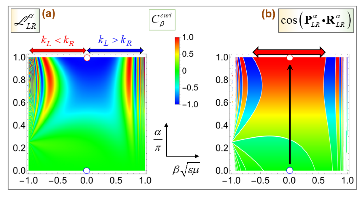
As with Figure 2, we present both $\left\{L_{LR}^{\alpha },\cos \left(P_{LR}^{\alpha }·R_{LR}^{\alpha }\right)\right\}$ in Figure 4 to see the effects of the rotation angle $\alpha$ the chirality parameter $\beta$ on the transition between asymmetry to symmetry. As in Figure 2a, we are handling only the curl-$\beta$-based constitutive relations $C_{\beta }^{curl}$ in Equation (3). Its counterpart for the field-$\kappa$-based constitutive relations $C_{\kappa }^{field}$ will not be much different as can be seen by comparing both panels of Figure 2. All input settings for Figure 4 are the same as those in Figure 2a. Added are $\left|Q_L\right|=\left|Q_R^{\alpha }\right|$ and $Z=1/2$ for evaluating $\cos \left(P_{LR}^{\alpha }·R_{LR}^{\alpha }\right)$ in Figure 4b.

In this regard, let us consider Equation (25) with two extreme types of materials with a specified $\epsilon \mu >0$: (i) $\left\{\epsilon ,\mu \right\}=\left\{\epsilon >0,1\right\}$ for a non-magnetic medium such that $\mathrm{sgn}\left(Z^{-1}-Z\right)=\mathrm{sgn}\left(\epsilon -1\right)=\mathrm{sgn}\left(\epsilon \mu -1\right)$, and (ii) $\left\{\epsilon ,\mu \right\}=\left\{1,\mu \right\}$ for a non-electric medium such that $\mathrm{sgn}\left(Z^{-1}-Z\right)=\mathrm{sgn}\left(1-\mu \right)=\mathrm{sgn}\left(1-\epsilon \mu \right)$. When assuming $\epsilon \mu >1$, $\mathrm{sgn}\left(Z^{-1}-Z\right)=\pm \mathrm{sgn}\left(\epsilon \mu -1\right)$ depending on either $\mu =1$ or $\epsilon =1$. We take $\mu =1$ for Figure 4 for concreteness so that $\mathrm{sgn}\left(Z^{-1}-Z\right)=\mathrm{sgn}\left(\epsilon \mu -1\right)=\mathrm{sgn}\left(4-1\right)=+1$ with a specified $\epsilon \mu =4$. Therefore, we try a nontrivial case with $Z\ne 1$.

Figure 4a is obtained by multiplying $\cos \left({\Gamma }_{LR}^{\alpha }+{\delta }_{LR}^{\alpha }\right)$ in Figure 2a through the factor $\frac{1}{2}\left(1-\cos \alpha \right)$. Therefore, we find in Figure 4a that $L_{LR}^{\alpha =0}=0$ on the lower boundary at $\alpha =0$. In comparison, $L_{LR}^{\alpha =\pi }=0$ on the upper boundary at $\alpha =\pi$ shows the same behavior as in Figure 2a.

We now turn to $\cos \left(P_{LR}^{\alpha }·R_{LR}^{\alpha }\right)$ in Equation (32). Let us take $\alpha =0$ and $\alpha =\pi$ in Equation (32) to obtain the following reduced formula for $\cos \left(P_{LR}^{\alpha =\pi }·R_{LR}^{\alpha =\pi }\right)$ with the assignment ${\delta }_{LR}^{\alpha }=0$.

$$\{\begin{array}{l}\cos \left(P_{LR}^{\alpha =0}·R_{LR}^{\alpha =0}\right)=0\\ \cos \left(P_{LR}^{\alpha =\pi }·R_{LR}^{\alpha =\pi }\right)=-\mathrm{sgn}\left[\cos \left({\Gamma }_{LR}^{\alpha =\pi }\right)\right]\end{array}$$

(33)

At $\alpha =0$, $\cos \left(P_{LR}^{\alpha =0}·R_{LR}^{\alpha =0}\right)=0$ corresponds the green color in Figure 4b. In comparison, $\cos \left(P_{LR}^{\alpha =\pi }·R_{LR}^{\alpha =\pi }\right)=-\mathrm{sgn}\left[\cos \left({\Gamma }_{LR}^{\alpha =\pi }\right)\right]$ at $\alpha =\pi$ from Equation (32). Therefore, $\cos \left(P_{LR}^{\alpha =\pi }·R_{LR}^{\alpha =\pi }\right)=\pm 1$ depending on $\beta$, as can be verified by either the true-red color or the true-blue color in Figure 4b at $\alpha =\pi$. Therefore, perfectly opposite flows in $\left\{P_{LR}^{\alpha =\pi },R_{LR}^{\alpha =\pi }\right\}$ are possible [36]. The symmetry of $\cos \left(P_{LR}^{\alpha =\pi }·R_{LR}^{\alpha =\pi }\right)$ with respect to $\beta =0$ is also easily seen in Figure 4b and by the behavior discussed for $\cos \left({\Gamma }_{LR}^{\alpha =\pi }\right)$ in Figure 2a and in Equation (26).

Let us perform numerical evaluations on the horizontal line at $\alpha =\pi$ in Figure 4b. We employ the formula ${\Gamma }_{LR}^{\alpha =\pi }=\left(k_L+k_R\right){\xi }_{-}$ from Equation (26) at $\alpha =\pi$ and the specified values of ${\xi }_{-}=\frac{1}{\sqrt{2}}$ and $\epsilon \mu =4$ with the help of $k_R+k_L={\left(1-{\beta }^2\epsilon \mu \right)}^{-1}2\sqrt{\epsilon \mu }$ from Equation (28) for $C_{\beta }^{curl}$. We thus have the following:

$${\Gamma }_{LR}^{\alpha =\pi }\left(\beta \right)=-\mathrm{sgn}\left[\cos \left(\frac{2\sqrt{\epsilon \mu }}{1-{\beta }^2\epsilon \mu }\frac{1}{\sqrt{2}}\right)\right]=-\mathrm{sgn}\left[\cos \left(\frac{2\sqrt{2}}{1-4{\beta }^2}\right)\right]$$

(34)

Of course, ${\Gamma }_{LR}^{\alpha =\pi }\left(0\right)=-\mathrm{sgn}\left[\cos \left(2\sqrt{2}\right)\right]=-\mathrm{sgn}\left(-0.951\right)>+1$. Meanwhile, the first incidence of the sign reversal away from $\beta =0$ takes place for ${\left(1-4{\beta }^2\right)}^{-1}2\sqrt{2}=\pi$, thus giving rise to numerical solution $\beta =\pm 0.158$. The resulting region of $-0.316\le \beta \sqrt{\epsilon \mu }\le +0.316$ on the plot scale is indicated by the horizontal red arrow over the top of Figure 4b. Positive and negative regions of $\cos \left(P_{LR}^{\alpha =\pi }·R_{LR}^{\alpha =\pi }\right)$ repeat themselves more frequently in the left and right regions in correspondence to higher modes of the cosine function [36].

Let us follow the vertical black arrow on the parametric plane of $\left\{\beta \sqrt{\epsilon \mu },\alpha /\pi \right\}$ in Figure 4b. With $\beta =0$ along this line, $\cos \left(P_{LR}^{\alpha }·R_{LR}^{\alpha }\right)=0$ at the lowest point with $\alpha =0$, thereby referring to an orthogonality between $\left\{P_{LR}^{\alpha },R_{LR}^{\alpha }\right\}$ for a co-propagating pair. As the oblique collision angle $\alpha$ is increased upward along this line, $\cos \left(P_{LR}^{\alpha }·R_{LR}^{\alpha }\right)$ is increased in magnitude as well, thus referring to a more anti-parallel alignment between $\left\{P_{LR}^{\alpha },R_{LR}^{\alpha }\right\}$. At $\alpha =\pi$ on the uppermost point, $\cos \left(P_{LR}^{\alpha }·R_{LR}^{\alpha }\right)=-1$, thus indicating a perfect anti-parallel alignment.

If $P_{LR}^{\alpha }·R_{LR}^{\alpha }=0$ holds true, the level lines of $P_{LR}^{\alpha }$ on the $xy$-plane would be orthogonal to those of $R_{LR}^{\alpha }$. Considering $R\equiv \mathrm{Im}\left(E\times H^{*}\right)$ and $R\equiv \mathrm{Im}\left(E\times H^{*}\right)$ in Equation (7), $E\times H^{*}\equiv P+iR$ would become an analytic function of complex variables if $P_{LR}^{\alpha }·R_{LR}^{\alpha }=0$. We have thus shown that such a complex analyticity is hardly achievable for generic oblique collisions. Instead, Figure 4b shows that $-1<\cos \left(P_{LR}^{\alpha }·R_{LR}^{\alpha }\right)<1$ over most of the $\beta \alpha$-plane. According to the color bar, Figure 4b confirms that $P_{LR}^{\alpha }·R_{LR}^{\alpha }=0$ (in green color) belong to a rare event that takes place only at $\alpha =0$. In comparison, symmetry with respect to $\beta$ is visible solely at $\alpha =\pi$.

6. Discussions

For lossless media with $\epsilon ,\mu >0$, $\left\{I,P,R\right\}$ and $\left\{I,C,K\right\}$ of Equations (6) and (7) admit the following boundedness properties via the Cauchy–Schwarz inequality [1,9,15,29,33,36].

$$I\equiv \frac{1}{2}\left(\epsilon E^{*}·E+\mu H^{*}·H\right),\begin{array}{c}\end{array}\{\begin{array}{l}I\ge \sqrt{\epsilon \mu }\left|E\times H^{*}\right|\equiv \sqrt{\epsilon \mu }\sqrt{{\left|P\right|}^2+{\left|R\right|}^2}\\ I\ge \sqrt{\epsilon \mu }\left|E·H^{*}\right|\equiv \sqrt{\epsilon \mu }\sqrt{C^2+K^2}\end{array}$$

(35)

Here, we recognize the importance of the relative light speed $c\equiv {\left(\epsilon \mu \right)}^{-1/2}$. Due to the complementary nature between $\left\{P,R\right\}$, the hot spots of the EM Poynting vector are roughly off the hot spots of the reactive Poynting vector [10,29]. A conventional inequality that $I\ge \sqrt{\epsilon \mu }\left|P\right|$ is not enough without consideration of its reactive counterpart $R$ [18]. Likewise, the complementary nature between $\left\{C,K\right\}$ suggests that the hot spots of the EM helicity are not likely to coincide with the hot spots of the reactive helicity [7]. A conventional inequality that $I\ge \sqrt{\epsilon \mu }\left|C\right|$ is not enough without consideration of its reactive counterpart $K$ [33].

To sum up, the symmetry between an EM parameter and a reactive parameter renders complete a boundedness property. This symmetry is another manifestation of the electric-magnetic democracy (or duality) [10,18,20]. This completeness has not been properly highlighted up until now.

Let us check how the first inequality of Equation (35) holds true to our obliquely colliding pair. This is easily seen that the specific inequality $\sqrt{\epsilon \mu }\sqrt{{\left|P_{LR}^{\alpha }\right|}^2+{\left|R_{LR}^{\alpha }\right|}^2}\le I_{LR}^{\alpha }$ is satisfied by combining $I_{LR}^{\alpha }$ from Equation (19) with $\left\{P_{LR}^{\alpha },R_{LR}^{\alpha }\right\}$ from Equation (24), while making use of $\left|\cos \left({\Gamma }_{LR}^{\alpha }+{\delta }_{LR}^{\alpha }\right)\right|\le 1$.

Likewise, combining Equations (21) and (24) for both helicities gives rise to the following steps.

$$\begin{array}{l}{\left(C_{LR}^{\alpha }\right)}^2+{\left(K_{LR}^{\alpha }\right)}^2={\left(Z^{-1}{\left|Q_L\right|}^2-Z{\left|Q_{LR}^{\alpha }\right|}^2\right)}^2+{\left[\left(1-\cos \alpha \right)\left|{\left(Q_L\right)}^{*}{Q}_R^{\alpha }\right|\cos \left({\Gamma }_{LR}^{\alpha }+{\delta }_{LR}^{\alpha }\right)\right]}^2\\ \begin{array}{c}\end{array}\le Z^{-2}{\left|Q_L\right|}^4+Z^2{\left|Q_R^{\alpha }\right|}^4-2{\left|Q_L\right|}^2{\left|Q_R^{\alpha }\right|}^2+4{\left|Q_L\right|}^2{\left|Q_R^{\alpha }\right|}^2={\left(Z^{-1}{\left|Q_L\right|}^2+Z{\left|Q_R^{\alpha }\right|}^2\right)}^2\end{array}$$

(36)

Resultantly, Equation (19) for the EM energy density leads to the desired inequality $\sqrt{\epsilon \mu }\sqrt{{\left(C_{LR}^{\alpha }\right)}^2+{\left(K_{LR}^{\alpha }\right)}^2}\le I_{LR}^{\alpha }$ [2,7]. We learn from the above series of steps that the equality is established under the more restrictive set of conditions that $\cos \alpha =-1$, $\left|{\left(Q_L\right)}^{*}{Q}_R^{\alpha }\right|=\left|Q_L\right|\left|Q_R^{\alpha }\right|$, and $\left|\cos \left({\Gamma }_{LR}^{\alpha }+{\delta }_{LR}^{\alpha }\right)\right|=1$. These three requirements correspond to a counter-propagating pair with a vanishing amplitude factor ${\delta }_{LR}^{\alpha }=0$. We can conclude from the Cauchy–Schwarz inequalities in Equation (35) that a pair of EM and reactive parameters are not only complementary but also complete. This notion of simultaneous complementarity and completeness has been largely overlooked in the existing literature [7].

In line with the first inequality in Equation (35), it is appropriate to find how much of the total energy density is divided, respectively, into the following three portions.

$$\frac{\sqrt{\epsilon \mu }\left|P_{LR}^{\alpha }\right|}{I_{LR}^{\alpha }},\frac{\sqrt{\epsilon \mu }\left|R_{LR}^{\alpha }\right|}{I_{LR}^{\alpha }},1-\frac{\sqrt{\epsilon \mu }\sqrt{{\left|P_{LR}^{\alpha }\right|}^2+{\left|R_{LR}^{\alpha }\right|}^2}}{I_{LR}^{\alpha }}$$

(37)

Since the medium chirality is normally very small, we have examined the resulting seven field properties in the limit of a small medium parameter, namely, $\left|\beta \sqrt{\epsilon \mu }\right|<<1$ or $\left|\kappa \right|<<\sqrt{\epsilon \mu }$ [3,28]. Such small medium chirality demands extreme sensitivities in sensing medium chiralities by measuring field helicities [42]. The symmetry in the signals acquired in response to the medium chirality would play an appropriate role in planning pertinent sensing experiments. Understanding gained in this study would be helpful to the shaping or fabrication of proper chiral media as well [28].

Consider for instance an inverse problem of deducing the medium chirality from the measured values of all or some of $\left\{I,J\right\}$ in Equation (6) and $\left\{P,R,C,K,M\right\}$ in Equations (7) and (12) [2,7,8]. In fact, we are not sure which pair of constitutive relations in Equation (3) are applicable to a medium at hand. Careful examination of the measured data will be of great help around the state near $\alpha =\pi$, namely, around the red boundary points in Figure 2. In this case, an evenness around $\beta =0$ and/or an independence on $\kappa$ will help to determine a correct pair of constitutive relations.

Recall that our problem stays essentially two-dimensional since we can always find a plane on which two colliding plane waves undergo propagations. Whenever more than three obliquely colliding waves are considered, we encounter in general three-dimensional situations [6]. In such three-dimensional configurations, the parameters so far found to vanish, say, $J_{LR}^{\alpha }=0$ in Equation (19), are highly likely to survive. In addition, other parameters would then become more complicated due to diverse possibilities of interferences. Such problems will make future topics of research.

Suppose that the angle $\alpha$ in $Q_R^{\alpha }$ of Equation (18) is considered spatially distributed along a certain straight line. A series of the resulting $Q_R^{\alpha }$ could then resemble the dynamics of the ‘phase-gradient geometric metasurfaces’ or simply ‘gradient metasurfaces’, where elemental units of structured metamolecules are arranged according to a predesigned orientation as in Equation (16). See Figure 60 in [25]. Our interference function ${\Gamma }_{LR}^{\alpha }\left(\alpha \right)$ in Equation (23) serves as a phase in $\cos \left({\Gamma }_{LR}^{\alpha }+{\delta }_{LR}^{\alpha }\right)$ of Equation (24). This function ${\Gamma }_{LR}^{\alpha }\equiv k_L{\xi }_{-}-k_R{\eta }_{-}$ is a sort of geometric phase although the oblique angle $\alpha$ is not geometric but more of a dynamic nature.

When a media under consideration is lossy, say, $\epsilon ,\mu \in ℂ$, almost all formulas handled in this study should be amended [2]. Spatially inhomogeneous properties, say, $\epsilon \left(x,y,z\right)$ and/or $\mu \left(x,y,z\right)$, would add more complexities [33]. Frequency-dispersive properties have also been worked out. Attendant interpretations would become complicated and require care [12,17,18,25]. In this aspect, $\tilde{\kappa }\left(\tilde{\omega }\right)$ could also be tackled in case with the ‘field-$\kappa$-based constitutive relations’ [24]. When asymmetrically shaped bodies immersed in an achiral medium are illuminated by circularly polarized plane waves, there should appear non-zero EM helicities [26]. Such Mie scatterings will make interesting hunting grounds for chiral optics [16].

In fluid mechanics, we find an interesting analogue to our problem. To this end, recall the simple inviscid Euler equations in a one-dimensional configuration, where a spatially dependent fluid velocity is given by $u\left(t,x\right)$. Meanwhile, the medium property manifests itself through a spatially dependent speed of sound $c\left(t,x\right)$. The usual pair of characteristics is given by $c\pm u$ so that the role of a medium chirality is played by $u\left(t,x\right)$ [36,39,41]. Here, the acoustic limit is given by the limit $\left|u\right|<<c$ as with our limit of small medium chirality, viz., $\left|\beta \sqrt{\epsilon \mu }\right|<1$ or $\left|\kappa \right|<\sqrt{\epsilon \mu }$. What we have presented in all of Figure 2, Figure 3, and Figure 4 correspond to the subsonic regime with $\left|u\right|<c$. In comparison, supersonic flows with $\left|u\right|>c$ are allowed in fluid mechanics, whereby various nonlinear issues of transitions and stability would come into play. In the future, we may explore such hypothetical transition phenomena that might take place over the critical point of either $\left|\beta \sqrt{\epsilon \mu }\right|=1$ or $\left|\kappa \right|=\sqrt{\epsilon \mu }$ [39]. We notice in this connection that a rather high value of $\kappa =0.85$ has been tested for an analytic investigation with $n\equiv \sqrt{\epsilon \mu }=3.5$ [7].

In fact, the problem formulation and its attendant solution presented in this section are rather simple in the sense that only a single unbounded chiral medium is under consideration. When an EM wave passes through two semi-infinite spaces occupied by a chiral medium and an achiral medium, respectively, there arise two distinct problems. Both problems will require enormous human efforts in making appropriate analysis in view of the complexity expounded by [30], even if the two media are separated by a planar interface.

We are looking into the behaviors of a plane incident wave as usual. Depending on where an incident and an accompanying reflected wave are located, the two problems are defined as follows. As the first problem, the ‘achiral-to-chiral (‘AC-to-C’ for short) problem is defined by the configuration, where an incident wave is illuminated from an achiral medium and a transmitted wave passes through a chiral medium. This AC-to-C problem has been extensively (but not completely) solved by [30]. As the second problem, the ‘chiral-to-achiral (‘C-to-AC’ for short) problem is defined by the configuration, where an incident wave is illuminated from a chiral medium and a transmitted wave passes through an achiral medium. This C-to-AC problem has never been solved as far as we are aware of.

The relative refractive indices of the two media do not affect the ensuing analysis to an appreciable degree except where a total internal reflection takes place. For simplicity, we continue to assume that the two media are loss-free. The two problems are certainly not space-invertible due to chiral constitutive relations. In other words, no reflection symmetry holds true between these two problems [27]. As a reference, the classical achiral-to-achiral (AC-to-AC) problem is defined by a configuration, where both semi-infinite media are dielectric with distinct positive refractive indices.

Let us make a brief review of the analytic solution for the first AC-to-C problem as presented in [30]. As usual, we can identify an incidence plane, whence a transverse-electric (TE) or s-wave and a transverse-magnetic (TM) or p-wave. An incident wave is here considered to be a linear combination of a TE-wave and a TM-wave. In the reference AC-to-AC problem, a TE-wave and a TM-wave are completely at our disposal, where we could arbitrarily combine them with a complex coherence factor. In comparison, the transmitted wave for the AC-to-C problem is normally a linear combination of the co-propagating pair $\left\{Q_L,Q_R^{\Rightarrow }\right\}$ listed in Equations (14) and (17) as dictated by the chiral medium. Resultantly, there is an inherent coupling between a TE-wave and a TM-wave employable for an incident wave.

Furthermore, let us mention that the first AC-to-C problem was investigated by [30] only with the field-$\kappa$-based constitutive relations $C_{\kappa }^{field}$ listed in Equation (4). Overall, algebraic manipulations involved in the first AC-to-C problem are unbearably complicated for ordinary impatient readers. For instance, a modified Brewster angle for this AC-to-C problem requires a long list of successive formulas. Notwithstanding, the key parameters $\left\{I,J\right\}$, $\left\{P,R\right\}$, and $\left\{C,K\right\}$ presented in Equations (6) and (7) have not been evaluated in both sides of the semi-infinite media. We expect that the evaluation of those key parameters involves a lot of algebra as well.

For the not-yet-solved second C-to-AC problem, an incident wave consists inherently of a linear combination of $\left\{Q_L,Q_R^{\Rightarrow }\right\}$. Notice that $\left\{Q_L,Q_R^{\Rightarrow }\right\}$ carry distinct wave numbers although their wave vectors are directed in an identical propagation direction [27]. The resulting reflected wave and transmitted wave should consist of two constituent waves. In other words, TE-TM or s-p interferences are inherent for this C-to-AC problem. There are still many fuzzy and unresolved aspects of this problem. This problem poses a variety of challenging tasks (both analytical and experimental) to us. For both problems, we might then be able to locate specific incidence angles where helicity neutralities prevail, i.e., $C=0$ and/or $K=0$ [10].

7. Conclusions

We have examined how a chiral medium responds to a pair of obliquely colliding plane waves. To this goal, we established a correct set of solutions to the Maxwell equations for a rotational pair of left and right waves. We have thus examined key bilinear parameters of energy densities, Poynting vectors, field helicities, and the spin angular momentum density. By evaluating these key parameters on the parametric plane of the medium chirality and the oblique rotation angle, we have shown that a collaborative and symmetric response can be obtained for a pair of counter-propagating plane waves. Ways of exploiting such symmetric properties are also suggested for a few applications.