Abstract
In this paper, we describe iterative derivative-free algorithms for multiple roots of a nonlinear equation. Many researchers have evaluated the multiple roots of a nonlinear equation using the first- or second-order derivative of functions. However, calculating the function’s derivative at each iteration is laborious. So, taking this as motivation, we develop second-order algorithms without using the derivatives. The convergence analysis is first carried out for particular values of multiple roots before coming to a general conclusion. According to the Kung–Traub hypothesis, the new algorithms will have optimal convergence since only two functions need to be evaluated at every step. The order of convergence is investigated using Taylor’s series expansion. Moreover, the applicability and comparisons with existing methods are demonstrated on three real-life problems (e.g., Kepler’s, Van der Waals, and continuous-stirred tank reactor problems) and three standard academic problems that contain the root clustering and complex root problems. Finally, we see from the computational outcomes that our approaches use the least amount of processing time compared with the ones already in use. This effectively displays the theoretical conclusions of this study.
MSC:
65H05; 49M15; 41A25
1. Introduction
There are many studies regarding the solution of nonlinear equations or systems; for example, see Traub [1], the first chapter of the book in Ref. [2], and the Refs. [3,4,5,6,7]. One of these studies involves finding multiple roots for a given nonlinear equation, which is the most demanding task; hence, various iterative algorithms have been suggested and studied by researchers [8,9,10,11,12,13,14] to find the simple and multiple roots of nonlinear equations. A root with a multiplicity of is called a multiple zero, also known as multiple points or a repeating root. Moreover, is called a simple zero. Solving a nonlinear equation with multiple zeros is a difficult task. In this article, we are interested in developing iterative algorithms for finding multiple root with a multiplicity of a nonlinear equation i.e., and .
In the literature [15,16], iterative algorithms using multiple steps (and points) to enhance the solution are referred to as multi-point iterations. In Ref. [15], the author presented a new Hermite interpolation-based iterative technique with a convergence order of , which requires, at each step, only two function evaluations. In Ref. [16], the author reviewed the Newton method’s most important theoretical results concerning the algorithm’s convergence properties, error estimates, numerical stability, and computational complexity.
Due to some interesting factors, many scholars have become interested in such algorithms. First, they can overcome the efficiency index of one-point algorithms, and second, multiple-step algorithms reduce the number of iterations and increase the order of convergence, reducing the computational load in numeric work. To find the multiple roots of a nonlinear equation, many scholars [17,18,19,20,21,22,23,24,25] developed higher-order iterative algorithms employing the first-order derivative. In the literature [17,18,20,21,22,24,25], researchers have developed optimal fourth-order methods requiring one function and two derivative evaluations per step. In Ref. [19], the authors presented six new fourth-order methods. The first four require one function and three-derivative evaluations per iteration, and the last two require one function and two derivative evaluations per iteration. In Ref. [23], the authors presented a class of two-point sixth-order multiple-zero finders with two functions and derivative evaluations per step.
The modified Newton’s method [26], which is defined as:
where is the multiplicity of root and is the first derivative of function , is one of the fundamental methods for finding multiple roots of a function. (1) has a quadratic convergence order if the multiplicity is known.
On the other hand, derivative-free algorithms to handle cases of multiple roots are extremely rare in contrast to the algorithms that require a derivative evaluation. The principle difficulty in developing derivative-free algorithms is studying their convergence order. For any complex problem, the derivative-free algorithms are important when the derivative of function is difficult to calculate or is expensive to evaluate. In the literature, to obtain the multiple roots of an equation using the second-order modified Traub–Steffensen technique [1], some authors [27,28,29,30,31,32,33,34] derived optimal derivative-free iterative algorithms. Now, the Traub–Steffensen technique [1] is given by:
Traub–Steffensen method (TM):
where , and . Without evaluating any derivatives, the modified Traub–Steffensen technique maintains its order of convergence.
Recently, Kumar et al. [30] and Kansal et al. [32] presented the second-order optimal schemes defined as:
Kumar method (M):
where is a weight function and .
Kansal method (KM):
where
So, constructing iterative methods with less function evaluation plays a key role. For this, optimal methods are introduced that satisfy the Kung–Traub conjecture [35]. Motivated by this, the goal of this work is to develop a method that can find multiple roots with the multiplicity . The salient feature of the proposed method is its simple body structure, which means no new evaluation of the function without the computation of the derivative. However, the main advantage of the proposed scheme is that it is equally suitable for both categories, viz., both simple and multiple roots. It demonstrates the generality of the proposed method.
The proposed work is divided into four sections. Section 2 includes the construction of a new scheme and a convergence analysis of the scheme. Some special cases of the new scheme are studied in Section 3, and stability is also verified in this section. Last, the conclusion is discussed in Section 4.
2. Development of Novel Scheme
Here, we present a new one-point algorithm of order two, requiring two (functional) evaluations per iteration. This means the proposed algorithm supports the Kung–Traub conjecture [35]. Let us consider the scheme for multiplicity ,
where the , , , , and parameters and are arbitrary.
The convergence of (5) is obtained by Theorems 1–3. First, we will discuss the case of in Theorem 1, in Theorem 2, and in Theorem 3. The study of the convergence analysis of scheme (5) is discussed in different parts because we will see the behaviour of the parameter as the multiplicity root of the function increase.
Theorem 1.
Let represent an analytical function in the vicinity of a simple zero (say, η) . Consider that initial guess is sufficiently close to η; then, the scheme defined by (5) has a second order of convergence, provided that and
Proof.
Let be the error in the q-th iteration. Using Taylor’s expansion of and about , and taking into account that and , we have
where , for . Using (6) and (7) in (5), we have
Equation (8) will have second order convergence if we set and Then, the final error Equation (8) is given by
Thus, the theorem is proved. □
Theorem 2.
Assume the hypothesis of Theorem 1 for multiplicity . Then, scheme (5) has a second order of convergence, provided that and
Proof.
Consider an error at the q-th iteration . Now, considering the expansion of and about by Taylor’s series, and taking into account that , , and , we have
where , for .
If we take , (12) becomes
In (13), we can see the parameter is present. So, making this error equation free from the parameter , we take . Then, error Equation (12) gives
Thus, the theorem is proved. □
Theorem 3.
Use the hypothesis of Theorem 1 for multiplicity . Then, scheme (5) has convergence order 2, provided that
Proof.
Taking into account that and , then, developing and about in the Taylor’s series, we get
where , for .
Take . Then, (17) becomes
Hence, the theorem is proved. □
Remark 1.
The presented scheme (5) reaches the second-order convergence provided that the conditions of Theorems 1, 2, and 3 are satisfied. This convergence rate is achieved by using only two function evaluations, viz., and , per iteration. Therefore, the scheme in Equation (5) is optimal according to the Kung–Traub hypothesis [35].
3. Numerical Results
In this section, the new algorithm NM is applied to solve some real-life practical problems, and to check the performance of the new algorithm, we apply the new algorithm NM for , , and . For numeric work, we denote the algorithm NM as NM1, NM2, and NM3 corresponding to , , and , respectively. To verify the theoretical order of convergence, we used the formula (see Ref. [36])
The performances of NM1, NM2, and NM3 are compared with a modified Traub–Steffensen method (2) and the Kansal et al. method (4). The considered method (4) is denoted by KM1, KM2, KM3, and KM4 for , and , respectively. These values of parameter a are the best for the numerical results, as argued in ref. [32].
All numerical problems given in Table 1 were performed with Mathematica 9 with stopping criterion . To check the performance of the presented algorithm, we display the (i) number of the iterations required, (ii) the last four differences between two consecutive iterations , (iii) the computational convergence order (COC) in Table 2, Table 3, Table 4, Table 5, Table 6 and Table 7, and (iv) the time consumption (CPU time) of methods in seconds to satisfy the criterion in Table 8.

Table 1.
The following numerical problems are considered for experimentation.
Table 2.
Performance of methods for problem 1.
Table 3.
Performance of methods for problem 2.
Table 4.
Performance of methods for problem 3.
Table 5.
Performance of methods for problem 4.
Table 6.
Performance of methods for problem 5.
Table 7.
Performance of methods for problem 6.
Table 8.
CPU time consumed by methods for considered problems (averages from 10 runs).
The computed results in Table 2, Table 3, Table 4, Table 5, Table 6 and Table 7 and Figure 1, Figure 2, Figure 3, Figure 4, Figure 5 and Figure 6 show that the suggested algorithms NM2 and NM3 exhibit good convergence characteristics in all considered problems, whereas in problem 1, the existing methods, namely KM1, KM2, KM3, and KM4, are not preserving their order of convergence. For problem 1, the efficient nature of the new methods is also displayed in Figure 1. In problem 2, the new methods NM1 and NM2 take less iterations for a particular initial guess for converging the required root, and the time consumption of all methods is shown in Figure 2, which shows the robust character of the new methods. In problem 3, we used D, which shows the diverging nature of the method. In problem 3, all considered methods, including the new method NM1, do not converge to the required root (except new methods NM2 and NM3 for a particular initial guess). Figure 3 explains the efficient character of new methods NM2 and NM3. Problems 4–6 and Figure 4, Figure 5 and Figure 6 also show the stability of the new methods. The increase in accuracy of the subsequent approximations, which is visible from the values of the differences , is the cause of the algorithm’s strong convergence. This also suggests that algorithms NM2 and NM3 are stable. Additionally, the accuracy of the approximations to solutions computed by the suggested algorithms is higher or equal to that of the approximations to solutions computed by the existing algorithms. The calculation of the convergence order, as shown in the last column in Table 2, Table 3, Table 4, Table 5, Table 6 and Table 7, verified the theoretical second order of convergence of the methods. Table 8, which shows that the CPU time is smaller than that of the CPU time used by existing algorithms, can also be used to assess the robustness of new algorithms (see Figure 4, Figure 5 and Figure 6). Many other different problems also confirm the stability of the new algorithms. Since the new methods use first-divided difference , a drawback of the method is that, if at some stage (say q) the denominator in the methods, then the methods may fail to converge. This section concludes that the new methods NM2 and NM3 are more stable and efficient.
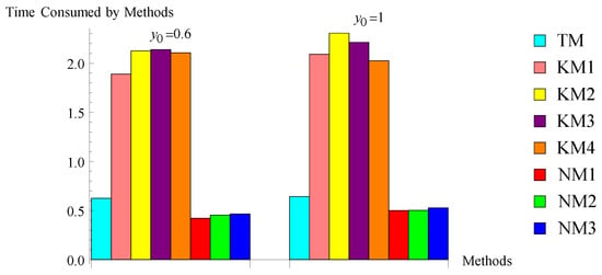
Figure 1.
Bar chart of problem .
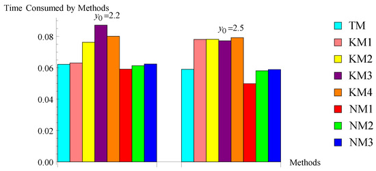
Figure 2.
Bar chart of problem .
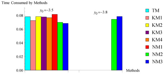
Figure 3.
Bar chart of problem .
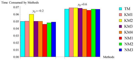
Figure 4.
Bar chart of problem .
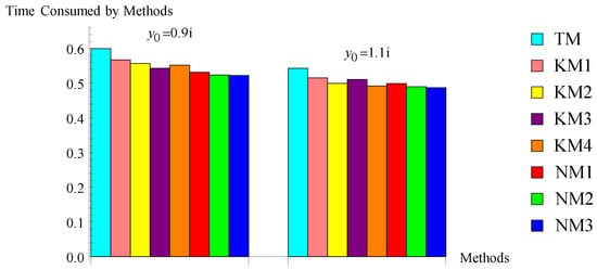
Figure 5.
Bar chart of problem .
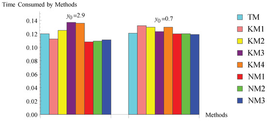
Figure 6.
Bar chart of problem .
4. Conclusions
The novel second-order optimal derivative-free family to find multiple roots of nonlinear equations is presented. Some new optimal methods are generated based on parameter . For comparison, the well-known modified Traub method is also taken into account. The order of convergence is examined. Additionally, by testing the proposed methods on some practical problems, the stability of the methods is confirmed. The efficient nature of the presented algorithms can be observed by the fact that the error is less than or equal to existing methods. The amount of CPU time consumed by the new methods NM2 and NM3 is less than that of the time taken by existing methods of the same nature. This shows the novelty of the presented algorithms. The main advantages of new algorithms NM2 and NM3 are that they are suitable for both categories, viz., simple and multiple roots. So, we conclude this study by remarking that the new algorithms NM2 and NM3 are good options for finding the simple and multiple roots of the equations.
Author Contributions
Conceptualization, methodology, S.K.; Formal analysis, validation, resources, L.J.; Software, writing—original draft preparation, J.B. All authors have read and agreed to the published version of the manuscript.
Funding
This research received no external funding.
Acknowledgments
We would like to express our gratitude to the anonymous reviewers for their help with the publication of this paper.
Conflicts of Interest
The authors declare no conflict of interest.
References
- Traub, J.F. Iterative Methods for the Solution of Equations; Chelsea Publishing Company: New York, NY, USA, 1982. [Google Scholar]
- Iliev, A.; Kyurkchiev, A.N. Nontrivial Methods in Numerical Analysis. In Selected Topics in Numerical Analysis; Lambert Academic Publishing: Chişinău, Moldova, 2010. [Google Scholar]
- Soleymani, F. Some optimal iterative methods and their with memory variants. J. Egypt. Math. Soc. 2013, 21, 133–141. [Google Scholar] [CrossRef]
- Hafiz, M.A.; Bahgat, M.S.M. Solving nonsmooth equations using family of derivative-free optimal methods. J. Egypt. Math. Soc. 2013, 21, 38–43. [Google Scholar] [CrossRef]
- Sihwail, R.; Solaiman, O.S.; Omar, K.; Ariffin, K.A.Z.; Alswaitti, M.; Hashim, I. A hybrid approach for solving systems of nonlinear equations using Harris Hawks optimization and Newton’s Method. IEEE Access 2021, 9, 95791–95807. [Google Scholar] [CrossRef]
- Sihwail, R.; Solaiman, O.S.; Ariffin, K.A.Z. New robust hybrid Jarratt-Butterfly optimization algorithm for nonlinear models. J. King Saud Univ.-Comput. Inform. Sci. 2022; in press. [Google Scholar] [CrossRef]
- Solaiman, O.S.; Hashim, I. Optimal eighth-order solver for nonlinear equations with applications in chemical engineering. Intell. Autom. Soft Comput. 2021, 27, 379–390. [Google Scholar] [CrossRef]
- Galantai, A.; Hegedus, C.J. A study of accelerated Newton methods for multiple polynomial roots. Numer. Algor. 2010, 54, 219–243. [Google Scholar] [CrossRef]
- Halley, E. A new exact and easy method of finding the roots of equations generally and that without any previous reduction. Philos. Trans. R. Soc. Lond. 1964, 18, 136–148. [Google Scholar]
- Hansen, E.; Patrick, M. A family of root finding methods. Numer. Math. 1977, 27, 257–269. [Google Scholar] [CrossRef]
- Neta, B.; Johnson, A.N. High-order nonlinear solver for multiple roots. Comput. Math. Appl. 2008, 55, 2012–2017. [Google Scholar] [CrossRef]
- Victory, H.D.; Neta, B. A higher order method for multiple zeros of nonlinear functions. Int. J. Comput. Math. 1983, 12, 329–335. [Google Scholar] [CrossRef]
- Akram, S.; Zafar, F.; Yasmin, N. An optimal eighth-order family of iterative methods for multiple roots. Mathematics 2019, 7, 672. [Google Scholar] [CrossRef] [Green Version]
- Akram, S.; Akram, F.; Junjua, M.U.D.; Arshad, M.; Afzal, T. A family of optimalEighth order iteration functions for multiple roots and its dynamics. J. Math. 2021, 2021, 5597186. [Google Scholar] [CrossRef]
- Frontini, M. Hermite interpolation and a new iterative method for the computation of the roots of non-linear equations. Calcolo 2003, 40, 109–119. [Google Scholar] [CrossRef]
- Galantai, A. The theory of Newton’s method. J. Comput. Appl. Math. 2000, 124, 25–44. [Google Scholar] [CrossRef]
- Sharifi, M.; Babajee, D.K.R.; Soleymani, F. Finding the solution of nonlinear equations by a class of optimal methods. Comput. Math. Appl. 2012, 63, 764–774. [Google Scholar] [CrossRef]
- Li, S.; Liao, X.; Cheng, L. A new fourth-order iterative method for finding multiple roots of nonlinear equations. Appl. Math. Comput. 2009, 215, 1288–1292. [Google Scholar]
- Li, S.G.; Cheng, L.Z.; Neta, B. Some fourth-order nonlinear solvers with closed formulae for multiple roots. Comput. Math. Appl. 2010, 59, 126–135. [Google Scholar] [CrossRef]
- Sharma, J.R.; Sharma, R. Modified Jarratt method for computing multiple roots. Appl. Math. Comput. 2010, 217, 878–881. [Google Scholar] [CrossRef]
- Zhou, X.; Chen, X.; Song, Y. Constructing higher-order methods for obtaining the multiple roots of nonlinear equations. J. Comput. Appl. Math. 2011, 235, 4199–4206. [Google Scholar] [CrossRef]
- Soleymani, F.; Babajee, D.K.R.; Lotfi, T. On a numerical technique for finding multiple zeros and its dynamics. J. Egypt. Math. Soc. 2013, 21, 346–353. [Google Scholar] [CrossRef]
- Geum, Y.H.; Kim, Y.I.; Neta, B. A class of two-point sixth-order multiple-zero finders of modified double-Newton type and their dynamics. Appl. Math. Comput. 2015, 270, 387–400. [Google Scholar] [CrossRef]
- Kansal, M.; Kanwar, V.; Bhatia, S. On some optimal multiple root-finding methods and their dynamics. Appl. Appl. Math. 2015, 10, 349–367. [Google Scholar]
- Behl, R.; Alsolami, A.J.; Pansera, B.A.; Al-Hamdan, W.M.; Salimi, M.; Ferrara, M. A new optimal family of Schröder’s method for multiple zeros. Mathematics 2019, 7, 1076. [Google Scholar] [CrossRef] [Green Version]
- Schröder, E. Über unendlich viele algorithmen zur Auflösung der gleichungen. Math. Ann. 1870, 2, 317–365. [Google Scholar] [CrossRef]
- Sharma, J.R.; Kumar, S.; Argyros, I.K. Development of optimal eighth order derivative-free methods for multiple roots of nonlinear equations. Symmetry 2019, 11, 766. [Google Scholar] [CrossRef]
- Sharma, J.R.; Kumar, S.; Jäntschi, L. On a class of optimal fourth order multiple root solvers without using derivatives. Symmetry 2019, 11, 1452. [Google Scholar] [CrossRef]
- Sharma, J.R.; Kumar, S.; Jäntschi, L. On derivative free multiple-root finders with optimal fourth order convergence. Mathematics 2020, 8, 1091. [Google Scholar] [CrossRef]
- Kumar, D.; Sharma, J.R.; Argyros, I.K. Optimal one-point iterative function free from derivatives for multiple roots. Mathematics 2020, 8, 709. [Google Scholar] [CrossRef]
- Kumar, S.; Kumar, D.; Sharma, J.R.; Cesarano, C.; Agarwal, P.; Chu, Y.M. An optimal fourth order derivative-free numerical algorithm for multiple roots. Symmetry 2020, 12, 1038. [Google Scholar] [CrossRef]
- Kansal, M.; Alshomrani, A.S.; Bhalla, S.; Behl, R.; Salimi, M. One parameter optimal derivative-free family to find the multiple roots of algebraic nonlinear equations. Mathematics 2020, 8, 2223. [Google Scholar] [CrossRef]
- Behl, R.; Cordero, A.; Torregrosa, J.R. A new higher-order optimal derivative free scheme for multiple roots. J. Comput. Appl. Math. 2021, 404, 113773. [Google Scholar] [CrossRef]
- Kumar, S.; Kumar, D.; Kumar, R. Development of cubically convergent iterative derivative free methods for computing multiple roots. SeMA 2022. [Google Scholar] [CrossRef]
- Kung, H.T.; Traub, J.F. Optimal order of one-point and multipoint iteration. J. Assoc. Comput. Mach. 1974, 21, 643–651. [Google Scholar] [CrossRef]
- Cordero, A.; Torregrosa, J.R. Variants of Newton’s method using fifth–order quadrature formulas. Appl. Math. Comput. 2007, 190, 686–698. [Google Scholar] [CrossRef]
- Danby, J.M.A.; Burkardt, T.M. The solution of Kepler’s equation. I. Celest. Mech. 1983, 40, 95–107. [Google Scholar] [CrossRef]
- Constantinides, A.; Mostoufi, N. Numerical Methods for Chemical Engineers with MATLAB Application; Prentice Hall PTR: Engle-Wood Cliffs, NJ, USA, 1999. [Google Scholar]
- Douglas, J.M. Process Dynamics and Control; Prentice Hall: Englewood Cliffs, NJ, USA, 1972; Volume 2. [Google Scholar]
- Zeng, Z. Computing multiple roots of inexact polynomials. Math. Comput. Lett. 2004, 74, 869–903. [Google Scholar] [CrossRef] [Green Version]
Publisher’s Note: MDPI stays neutral with regard to jurisdictional claims in published maps and institutional affiliations. |
© 2022 by the authors. Licensee MDPI, Basel, Switzerland. This article is an open access article distributed under the terms and conditions of the Creative Commons Attribution (CC BY) license (https://creativecommons.org/licenses/by/4.0/).