The QCD Adler Function and the Muon g − 2 Anomaly from Renormalons

Abstract

We describe the Adler function in Quantum Chromodynamics using a transseries representation within a resurgent framework. The approach is based on a Borel-Ecalle resummation of the infrared renormalons combined with an effective running for the strong coupling. The new approach is flexible enough to give values in agreement with the current Adler function determinations. We then apply our finding to the muon’s anomalous magnetic moment studying the possibility of saturating, solely in terms of the vacuum polarization function, the current discrepancy between the best Standard Model value for the muon’s anomalous magnetic moment and the experimental value obtained by the most recent muon $g-2$ collaboration. The latter shows that the Adler function’s new representation can also be consistent with recent lattice determinations.

1. Introduction

The Quantum Chromodynamics (QCD) description at the hadronic scale is a formidable challenge due to the breakdown of the perturbation theory description for finite values of the coupling constant. Currently, perturbation theory is the only analytical tool to compute physical quantities within quantum field theory (QFT). The Adler function [1] is a fundamental quantity used in QCD to describe the nonperturbative effects at the hadronic scale. Its perturbative expression is known for up to five loops [2]. Its theoretical description is essential since it appears in any process involving QCD corrections due to the vacuum hadronic polarization function. Lattice QCD allows performing a nonperturbative treatment of the QCD Adler function at the hadronic scale [3]. However, analytic, nonperturbative solutions are hard or impossible to obtain within the lattice framework. Hence, an analytical understanding would be beneficial. Based on the notion of renormalons [4,5,6,7] and Operator-Product-Expansion [8,9], there are non-perturbative analytical evaluations for the Adler function and QCD observables [10,11,12,13]. Other methods use integral representations [14,15,16]. Although all these analytical approaches reproduce some qualitative features of the “experimental” Adler function [17], the description is insufficient to describe the experimental data at the hadronic scale.

The recent analytical approach to the Adler function of Ref. [18] distinguishes itself from previous ones because it is based on renormalons and the resurgence theory. First proposed by Ecalle [19] in a purely mathematical context, it has found fertile ground in QFT [20,21,22,23,24,25,26,27,28,29]. Renormalized perturbation theory controls the finiteness of QFT in the proper regime. Therefore, it is an appealing possibility to continue it to the nonperturbative regime analytically. For this reason, resurgence may represent a good candidate for a foundational, analytical approach to a nonperturbative QFT.

In the specific framework of ordinary-differential-equations [30,31] (ODEs), a resurgent approach to the renormalization group was proposed in Refs [32,33]. The renormalization group equation (RGE) in this new approach is written as a non-linear ODE in the coupling constant. The resulting theory is then applied to the QCD Adler function [18], where the renormalons can be resummed, leaving one arbitrary constant fixed from data. It represents an improvement to all the known renormalon-based evaluations in QFT and QCD. The inability to calculate this arbitrary constant is due to the non-existence of a semiclassical limit for renormalons. Because of the technical details we shall discuss, the transseries representation for the Adler function has three arbitrary constants to be determined from the data.

In this work, we show that the new approach of Ref. [18] has the flexibility to reproduce the Adler function data in the entire infrared (IR) regime, provided that one properly regularizes the Landau pole [34] singularity. To this aim, we adopt an effective running for the strong coupling ${\alpha }_s$ that prevents the coupling from diverging [35]. The nonperturbative running we adopt is such that the strong coupling freezes at low energy [36]—see the review [37] for typical nonperturbative running for ${\alpha }_s$. The final result is shown in Figure 1. Our result features three parameters in contrast to conventional renormalon approaches with an infinite number of arbitrary constants. To illustrate the predictivity of the transseries representation, we also compare it with a fit including the same number of free parameters (three) but in conventional renormalon-based evaluation. In this case, there is no agreement between the theory and data for energies below ≈1.3 GeV.

We then apply the new tool to the $g-2$ discrepancy [38,39]. In particular, we follow the possibility considered in Ref. [40], in which the QCD vacuum polarization function is tentatively modified below ∼0.7 GeV because this is not yet excluded at that energy to saturate the $g-2$ discrepancy. The latter would agree with the most recent experimental result obtained by the $g-2$ collaboration [41] and the most recent lattice computation [42]. From the proposed approach’s perspective, we study the impact of the transseries representation of the Alder function on the anomalous magnetic moment of the muon.

2. The Adler Function

The Adler function $D\left(Q\right)$ is defined as

$$D\left(Q\right)=4{\pi }^2{Q}^2\frac{\mathrm{d}\mathsf{\Pi }\left(Q\right)}{\mathrm{d}{Q}^2},$$

(1)

where $\mathsf{\Pi }\left(Q\right)$ is determined via

$$\begin{array}{cc}\hfill -\mathrm{i}\int d^{4}x& {\mathrm{e}}^{-iqx}〈0\left|T\left(j_{\mu }\left(x\right)j_{\nu }\left(0\right)\right)\right|0〉\hfill \\ \hfill & =\left(q_{\mu }{q}_{\nu }-q^2{g}_{\mu \nu }\right)\mathsf{\Pi }\left(Q\right),\hfill \end{array}$$

(2)

being q the transferred momentum, $Q^2=-q^2$ and $j_{\mu }=\overline{q}{\gamma }_{\mu }q$ two massless quark currents. In perturbation theory, the Adler function is given by

$$D_{pert}\left(Q\right)=1+\frac{{\alpha }_s}{\pi }\sum _{n=0}^{\infty }{\alpha }_s^n\left[d_n{\left(-{\beta }_0\right)}^n+{\delta }_n\right].$$

(3)

We use the convention for the beta function $\beta \left({\alpha }_s\right)={\mu }^2\frac{d{\alpha }_s}{d{\mu }^2}={\beta }_0{\alpha }_s^2+{\beta }_1{\alpha }_s^3+\mathcal{O}{\left({\alpha }_s\right)}^4$, $2\pi {\beta }_0=-11+\frac{2}{3}{n}_f$, where $n_f$ is the number of active flavors, ${\alpha }_s=g_s^2/4\pi$ and $g_s$ denotes the gauge coupling of the strong interaction gauge group $SU{\left(3\right)}_c$. The Adler function expression in perturbation theory up to $n=2$ can be found in Refs. [10,43,44,45], from which the coefficients $d_n$ and ${\delta }_n$ can be extracted, as shown in Ref. [10]. The five-loop coefficient $d_3$ and ${\delta }_3$ can be extracted from Ref. [2]. Notice that in Equation (3) one needs to know the all coefficients $d_n$ and ${\delta }_n$ up to $n\to \infty$. As we discussed, it is only possible to compute the first few orders in perturbation theory expansions. Fortunately, there is a well-known procedure in the literature called “Naive non-abelianization” [10,46], which is used to estimate Equation (3) to all orders in perturbation theory. Essentially, within this procedure, one estimates the large order behavior in Equation (3) using the first know coefficients $d_n$ and ${\delta }_n$ from perturbation theory. The remaining coefficients are then estimated using the property that $d_n\propto n!$ whereas ${\delta }_n$ is not, so that for sufficiently large n one has ${\delta }_n/d_n\to 0$. As a crude approximation, one then sets the coefficients ${\delta }_n$ to zero for $n\ge 4$. This procedure is expected to give more accurate results as new perturbative computations are included. Finally, the coefficients $d_n$ for $n\ge 4$ are estimated from the fermion renormalons graphs computed in Ref. [10].

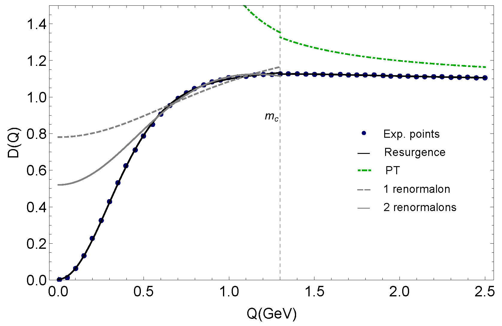
3. Resurgent Adler Function

In Ref. [18], we resummed the IR renormalon contribution to the QCD Adler function using the Borel-Ecalle resummation of Refs. [32,33]—see the Appendix A, Appendix B and Appendix C for more details on the resurgent approach. After resuming the renormalons using the new framework, the expression for the Adler function features three arbitrary constants: one constant $c_1$ parametrizing simple pole ambiguity due to the first non-zero renormalon; another constant C stemming from the Borel-Ecalle resummation of quadratic renormalons; a constant K related to the $n!$ behavior in the perturbative series [10], which in the case of renormalons and unlike instantons [47], cannot be determined using semiclassical methods [6]. The inability to determine those constants from first principles is a well-known problem. It has been recently linked to foundational issues to construct an unambiguous QFT starting from the free fields [48].

The original fermion bubble graph contribution to the Adler function was calculated in Ref. [49]. In Ref. [18], we rewrote the fermion bubble graph contribution of Ref. [49] such that the pole structure of the Borel transform was apparent. After applying the Borel-Ecalle resummation of Refs. [32,33], the transseries expression of the Adler function is of the form.

$$\begin{array}{cc}\hfill D_{resurg.}\left(Q\right)=& D_0\left(Q\right)-\frac{4\pi }{{\beta }_0}{c}_1{e}^{\frac{2}{{\beta }_0{\alpha }_s\left(Q^2\right)}}\hfill \\ \hfill & +C{e}^{\frac{1}{{\beta }_0{\alpha }_s\left(Q^2\right)}}{\left(\frac{1}{{\alpha }_s\left(Q^2\right)}\right)}^{a_p}{D}_1\left(Q^2\right),\hfill \end{array}$$

(4)

where $a_p=1+\mathcal{O}({\beta }_1/{\beta }_0^2)$. The function $D_0\left(Q\right)$ contains the perturbative expression up to $\mathcal{O}\left({\alpha }_s^4\right)$ shown in Equation (3) and is given by:

$$D_0\left(Q\right)=D_{pert}\left(Q\right)+D_K\left(Q\right),$$

(5)

where $D_K\left(Q\right)\propto {\sum }_{n=0}^{\infty }K{\beta }_0^n{\alpha }_s^{n+1}n!$. Following the formalism of Ref. [31], we then regularize the $n!$ divergence in $D_K$ by taking the Cauchy principal value for the Laplace integral such that

$$\begin{array}{cc}\hfill \frac{D_K\left(Q\right)}{2K}& =\frac{e^{\frac{2}{{\alpha }_s{\beta }_0}}\mathsf{\Gamma }\left(0,\frac{2}{{\alpha }_s{\beta }_0}\right)}{{\beta }_0}+\frac{2e^{\frac{3}{{\alpha }_s{\beta }_0}}\mathsf{\Gamma }\left(0,\frac{3}{{\alpha }_s{\beta }_0}\right)}{3{\alpha }_s{\beta }_0^2}+\hfill \\ \hfill & \sum _{p=1}^{\infty }\left(\frac{{\alpha }_s{\beta }_0-2(p+1)e^{\frac{2(p+1)}{{\alpha }_s{\beta }_0}}\mathsf{\Gamma }\left(0,\frac{2(p+1)}{{\alpha }_s{\beta }_0}\right)}{3{\beta }_0^2{\alpha }_{s}p(p+1)(2p+1)}+\right.\hfill \\ \hfill & \left.\frac{2\left((2p+3)e^{\frac{2p+3}{{\alpha }_s{\beta }_0}}\mathsf{\Gamma }\left(0,\frac{2p+3}{{\alpha }_s{\beta }_0}\right)-{\alpha }_s{\beta }_0\right)}{3{\beta }_0^2{\alpha }_s(p+1)(2p+1)(2p+3)}\right).\hfill \end{array}$$

(6)

In the above expression, the terms up to $\mathcal{O}\left({\alpha }_s^4\right)$ must be removed in $D_K\left(Q\right)$ to prevent the double counting of this contribution in $D_{pert}\left(Q\right)$. The Equation (6) is derived in the Appendix C.

Finally, the function $D_1\left(Q^2\right)$ is found from $D_0$ [32] using resurgence as shown in Refs. [32,33]. Choosing the renormalization scale ${\mu }^2=Q^2{e}^{-5/3}$ and neglecting the two-loop corrections proportional to ${\beta }_1$, one finds (We also proved that Equation (A26) could be derived using Ecalle bridge equation obtained from the RGE. We will discuss the latter point in a separate publication).

$$\begin{array}{cc}\hfill D_1\left(Q\right)& =\frac{8\pi K}{3{\alpha }_s{\beta }_0^2}\left[2e^{\frac{1}{{\alpha }_s{\beta }_0}}-\left(e^{\frac{1}{{\alpha }_s{\beta }_0}}+1\right)log\left(1-e^{\frac{2}{{\alpha }_s\beta 0}}\right)\right.\hfill \\ & -\left.2\left(e^{\frac{1}{{\alpha }_s\beta 0}}+1\right){tanh}^{-1}\left(e^{\frac{1}{{\alpha }_s{\beta }_0}}\right)\right].\hfill \end{array}$$

(7)

The next step is implementing the nonperturbative running for the coupling ${\alpha }_s\left(\mu \right)$ to be used in Equation (4).

4. Effective Running and the QCD Adler Function at Low Energies

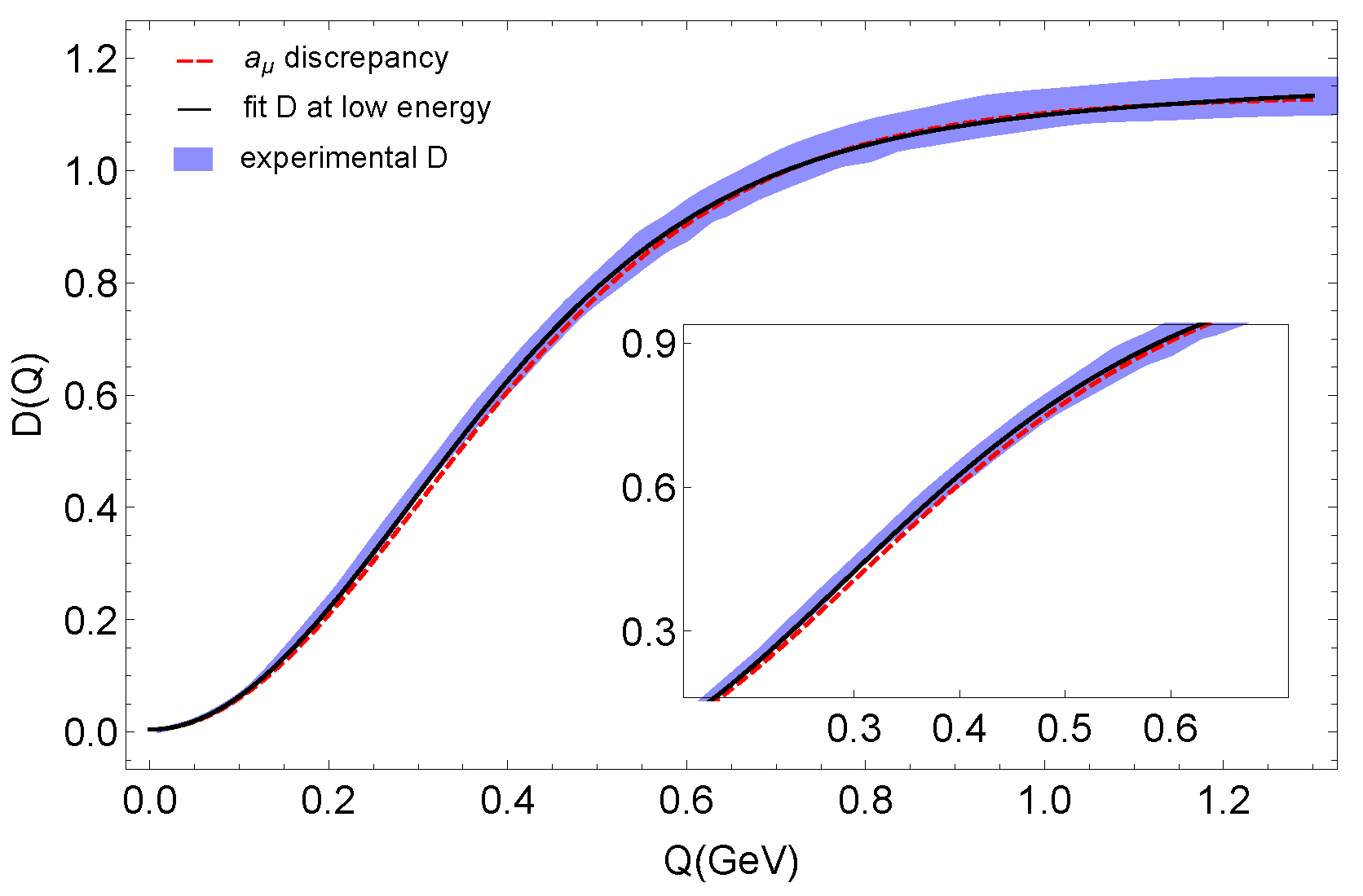
In Ref. [50], the authors explored the possibility that the QCD running coupling can be effectively extrapolated in a process-independent way to smaller momenta of the order of the hadronic scale. The essential idea is that nonperturbative physics should reveal itself smoothly in inclusive observables. Consequently, it is meaningful to extend the notion of the QCD coupling ${\alpha }_s$ down to zero energy for these types of observables. These arguments apply to the QCD Adler function as well.

The transseries provided in Ref. [18] can fit the experimental Adler function up to energy ≈0.7 GeV. The failure below that energy is due to the unphysical Landau pole of the perturbative running of ${\alpha }_s$—and not the Borel-Ecalle resummation formalism. To overcome this difficulty, in this work, we use an effective running coupling valid up to zero energy in which ${\alpha }_s$ goes to a constant value at zero energy. We should stress here that, in this case, the absence of the IR Landau pole is not in contradiction with the presence of the renormalons and their Borel-Ecalle resummation in Equation (4). The correspondence between the Landau pole and renormalons only holds at the perturbative level. In particular, the renormalons are calculated using the one-loop $\beta -$function. The renormalons only signal the nonperturbative energy scale $\mathsf{\Lambda }$ at which perturbation theory breaks down, as initially discussed in Ref. [51] and elaborated, among others, in Refs. [52,53]. More recently, the issue has been analyzed with the resurgence of the RGE, taking the ${\varphi }^4$-model as a prototype [54], where the possibility that non-analytic corrections from renormalons make the model asymptotically safe is argued (The avoidance of Landau pole via non-analytic (flat) contributions was previously discussed in Ref. [55]).

In our specific case, we use Cornwall’s coupling [35], which is one of the simplest analytic nonperturbative models for the running of ${\alpha }_s$ and given by [36]

$${\alpha }_s\left(Q\right)=\frac{4\pi }{11ln\left(z+{\chi }_g\right)-2n_{\mathrm{f}}ln\left(z+{\chi }_q\right)/3},$$

(8)

where $z=Q^2/{\mathsf{\Lambda }}^2$, $n_f$ is the number of flavors, ${\chi }_g=4m_g^2/{\mathsf{\Lambda }}^2$, ${\chi }_q=4m_q^2/{\mathsf{\Lambda }}^2$, the light constituent quark mass $m_q=350$ MeV, the gluon mass $m_g\simeq 500$ MeV, and $\mathsf{\Lambda }$ denotes the QCD hadronic (non-perturbative) scale. We shall determine $\mathsf{\Lambda }$ by fitting the experimental data of the Adler function.

A comment is now in order. Our approach provides a representation of the QCD Adler function as a transseries in ${\alpha }_s$, and the only requirement for Equation (4) to hold is that the coupling is not too large [18]. The perturbative and the effective couplings coincide in the UV, where they are sufficiently small for the Equation (4) to be valid. Therefore, an effective top-bottom running of Equation (4) is performed through Equation (8).

Notice also that, based on the (resummation of) renormalons, the result is intrinsically effective because of the inability to determine the parameters $K,C,c_1$. Therefore, the use of Equation (8) for describing the low-energy running of ${\alpha }_s$ brings in no additional conceptual changes (The operation of power corrections to physical observables and make the coupling ${\alpha }_s$ effective (analyzation) do not commute, and this would lead to ambiguity in Equation (4) [56,57,58]. However, since Equation (4) is intrinsically ambiguous, one can reabsorb the ambiguity mentioned above in the definition of the fitted parameters (e.g., “$C$”)). We find that the typical running for ${\alpha }_s$ reproducing the Adler function is such that at low energies, ${\alpha }_s\left(0\right)\simeq 1.6$, which is in the ballpark of known results in the literature. See Ref. [37] and references therein for a detailed discussion about the low energy behavior of the QCD running coupling in several nonperturbative approaches. The possibility of describing the nonperturbative running of ${\alpha }_s$ within the resurgent framework merits dedicated analysis and is therefore left for future work.

In

Table 1. Numerical value of the constants in Equation (4). The central column represents the low energy ($Q\lesssim 1.3$ GeV) fit, starting from the four-loop perturbative expression. The third column shows the values starting from the five-loop perturbative expression, corresponding to the plot in Figure 1.

Parameter	Low Energy Fit (4-Loop)	Low Energy Fit (5-Loop)
K	1.422	0.805
C	0.629	0.240
$c_1$	0.0326	−0.358
$\mathsf{\Lambda }$	731 MeV	697 MeV

, we show the values for the parameters entering in the transseries for the Adler function in Equation (4). We show the values obtained from the fit using the four-loop and five-loop expressions for the Adler function and find agreement with the current determinations of the QCD Adler function in both cases. However, as seen from the table, there is a significant difference in the numerical values for the constants $K,C,c_1$. These variations estimate the theoretical uncertainties for these constants, which we find to be at least ∼$100\%$. We interpret the large errors as the need to include higher-order perturbative corrections: more perturbative information would correspond to convergent values of the parameters. This is not surprising since the entire resurgent approach developed in Refs. [18,33] starts, by construction, from perturbation theory, which needs to be known at all orders in ${\alpha }_s^n$. In practice, this is not the case, and it is the theoretical reason behind the large theoretical uncertainties for the transseries parameters reported in Table 1.

With this in mind, we show in Figure 1 the Adler function in the energy range $Q=(0,2.5)$ GeV using the five loop expression for the Adler function. We see no appreciable difference at energies $Q=(1.3,2.5)$ GeV between the expressions coming from the first two power corrections (gray lines) and the resurgent result (solid black line). Conversely, in the low energy range $Q=(0,1.3)$ GeV, the solid and dashed gray lines fail to describe the Adler function, while the solid black line successfully follows the behavior of the data in the whole range. Despite the significant uncertainties previously discussed, to our knowledge, this is the first time the resurgence formalism provides a phenomenological result for QCD, in particular, an expression for the Adler function that can be used at all energies.

5. Saturating the $\mathit{g}-\mathbf{2}$ Experimental Discrepancy of the Muon Anomalous Magnetic Moment of the Muon

We consider now the so-called hadronic vacuum polarization (h.v.p.) contribution to the magnetic moment of the muon $\overrightarrow{\mu }$—for analyses on this subject see Refs. [38,39,59,60,61,62,63,64,65]. It is given by

$$\overrightarrow{\mu }=g\frac{Q_e}{2m_{\mu }c}\overrightarrow{s},$$

(9)

where $\overrightarrow{s}$ is the spin, $Q_e$ is the electric charge, $m_{\mu }$ is the muon mass, c is the speed of light, and Dirac’s theory predicts $g=2$. Quantum effects correct the value $g=2$ and the deviation is parameterized as $a_{\mu }=(g-2)/2$. Comprehensive analyses of muon $g-2$ within the Standard Model can be found in Refs. [64,66,67,68].

The leading order hadronic vacuum polarization contribution in terms of the QCD Adler function is of the form [61,69]

$$a_{\mu }^{\left(\mathrm{h}.\mathrm{v}.\mathrm{p}.\right)}=2{\pi }^2{\left(\frac{\alpha }{\pi }\right)}^2{\int }_0^1\frac{dx}{x}(1-x)(2-x)D\left(Q\right),$$

(10)

where $\alpha \simeq 1/137$ is the electromagnetic coupling constant, and $Q=\sqrt{\frac{x^2}{1-x}{m}_{\mu }^2}$.

Although the numerical instabilities for the parameters discussed in the previous section, it is worth asking whether our model can implement the tentative idea proposed in Ref. [40]. The authors studied the possibility that the $g-2$ discrepancy could be solely explained by modifying the SM vacuum polarization function contribution, deeming this scenario rather unlikely. A modification of the h.v.p. can be in tension with electro-weak precision tests [70,71] (Constraints on the h.v.p. are also discussed in Ref. [72]. Direct measurement of the h.v.p. will definitively shed light on the subject [73].) Although improbable, the authors of Ref. [40] still noted that there might be a missed contribution for $Q\lesssim 0.7$ GeV, an energy range in which constraints do not yet rule out the possibility of explaining the $g-2$ discrepancy by deviations of the $e^{+}{e}^{-}$ cross-section measurement. Interestingly, this would be consistent with the most recent lattice evaluation [42].

We wish to consider the impact of this hypothesis on our model. Thus we require the Adler function to match the experimental data for energies $Q\ge 0.7$ GeV and instead to allow for some deviations below $Q<0.7$ GeV.

The integral in Equation (10) requires the Adler function $D\left(Q\right)$ in the energy range $[0,\infty )$. Following Ref. [17], one has to split D in two branches, using the perturbative estimate for $Q>\sqrt{1.6}$ GeV and the data for $⩽\sqrt{1.6}$ GeV. The Equation (4) provides a good estimate of data. Thus the Adler function used in the evaluation of Equation (10) is given by

$$D\left(Q\right)=\left\{\begin{array}{cc}{D}_{resurg.}\left(Q\right)\hfill & Q⩽\sqrt{1.6}\mathrm{GeV}\hfill \\ D_{pert.}\left(Q\right)\hfill & Q>\sqrt{1.6}\mathrm{GeV}.\hfill \end{array}\right.$$

(11)

The corresponding behavior of the Adler function in $[0,1.3]$ GeV is shown in Figure 2 (solid black line), together with the experimental uncertainties represented by the light blue band.

The modification of the value of the constants K, $c_1$ and C, shown in

Table 2. Values reproducing the experimental $g-2$ discrepancy.

Parameter	${\mathit{a}}_{\mathit{\mu }}$ Discrepancy
K	0.865
C	0.764
$c_1$	−0.184
$\mathsf{\Lambda }$	677 MeV

, saturates the gap between the average value of $a_{\mu }^{\left(\mathrm{h}.\mathrm{v}.\mathrm{p}.\right)}\simeq 6.9\times {10}^{-8}$ [38,39] and the value $a_{\mu }^{\left(\mathrm{h}.\mathrm{v}.\mathrm{p}.\right)}\simeq 7.15\times {10}^{-8}$ consistent with the Muon $g-2$ Collaboration [41] experimental result. The deviations with respect the values in Table 1 (third column) are about few percent for K and $\sim 100\%$ for C and $c_1$. Notice that the deviations are outside the range estimated in the previous section varying the starting perturbative information. This is expected since, by construction, we are now describing a modified Adler function, such that it is in agreement with $a_{\mu }$ measurement and no longer the current “experimental” one in Figure 1. The plot for the Adler function, corresponding to the values for $C,c_1$ and K in Table 2, is shown in Figure 2 represented with the dashed red line.

In our picture the deviation concerning the average value $a_{\mu }\simeq 6.9\times {10}^{-8}$ of Refs. [38,39] is due to non-perturbative (non-analytic) contributions in the strong coupling constant ${\alpha }_s$, which were calculated using the resurgence framework of Refs [32,33]. These non-analytic contributions become dominant for ${\alpha }_s$∼1. The nonperturbative electro-weak corrections are sub-leading since the numerical values of the electromagnetic and weak couplings remain small at the muon mass-energy scale.

6. Summary and Outlook

We have shown that the analytical expression for the Adler function in Equation (4) has the flexibility to reproduce the Adler function data at the hadronic scale within the range of current determinations. We have used Cornwall’s coupling to model the running of ${\alpha }_s$ whose value freezes at low energies with ${\alpha }_s\left(0\right)$∼$\mathcal{O}\left(1\right)$. In this work, we focused on the latter effective description for the running of ${\alpha }_s$ due to its simplicity. Cornwall’s coupling ensures the applicability of the resurgent approach to renormalons and renormalization group equation of Ref. [33], which relies on non-linear, ordinary differential equations [31]. As a result, Equation (4) features 3 + 1 arbitrary parameters ($K,C,c_1$ and $\mathsf{\Lambda }$), in contrast to conventional renormalon-based evaluations with an infinite number of arbitrary constants.

We have determined those parameters from data, shown in Table 1, and our representation of the Adler function is drawn in Figure 1. At the present level, our method is not yet quantitatively stable; namely, the values of the fitted parameters are sensitive to the perturbative information that one starts with—as expected. There is the possibility that the knowledge of higher-loop corrections for the Adler function would stabilize the values for the parameter shown in Table 1. However, one potential problem against this possibility is that the coefficients ${\delta }_n$ in Equation (3) also receive $n!$ contributions independent from the renormalons due to the instantons, related to the proliferation of the number of Feynman diagrams as the order of perturbation theory $\mathcal{O}\left({\alpha }_s^n\right)$ increases. This means there are two superimposed Stokes lines, one due to the renormalons and the other due to the instantons. This situation is often called “resonance” in the mathematical literature. The treatment of renormalons, proposed here and the previous Refs. [18,33], is in the approximation of non resonance, as also assumed in Ref. [31]. Giving up on this assumption leads to a complex mathematical challenge of considering the instantons on top of the renormalons, and to our knowledge, this is an open mathematical problem. However, since renormalons induce the nearest singularity from the origin of the Borel plane, they dominate the large order behavior of the perturbative expansion [7] as long as the coupling ${\alpha }_s$∼1. We speculate that the non-resonant effects from instanton and renormalon singularities might give a subleading contribution that would not drastically modify our conclusions.

Notwithstanding the above sources of theoretical uncertainties, the IR description of the Adler function provided by resurgence gives a remarkable improvement to standard analytical approaches—with an infinite number of arbitrary constants. Still, we have not addressed the impact on the $K,C,c_1$ and $\mathsf{\Lambda }$ from the inclusion of the chiral symmetry-breaking effects due to quark masses. However, we expect the uncertainties due to the perturbative inputs in Table 1 to be the dominant ones, and these issues are left for future work. The interplay with different processes would open the possibility of testing the universality of QCD running coupling and of the constants in Table 1, in the spirit of Ref. [50]. Indeed, we expect our result to apply to other relevant processes involving the two-point Green function at the hadronic scale. An example may be the event shape observables in $e^{+}{e}^{-}$ collisions [75,76,77,78,79,80]. Other applications may be on the determination of the heavy quark pole mass [81,82] and on the static quark-antiquark potential [83].

We have also addressed the implications and the interplay with the muon’s magnetic moment. In particular, we implemented in our model the tentative hypothesis to explain the SM discrepancy for $a_{\mu }$ [41] by modifying the vacuum-hadronic-polarization contribution. As shown in Figure 2, its only effect is slightly spoiling the behavior of the Adler function at energies $\lesssim 0.7$ GeV, a range in which data may not be complete due to missed contributions in the hadronic cross-section $\sigma (e^{+}{e}^{-}\to hadrons)$. The corresponding modification of the (fitted) parameters that would explain the $g-2$ discrepancy is shown in Table 2. As proof of concept, our result implies that the muon $g-2$ discrepancy can be accounted for by including non-analytic contributions in the strong coupling constant ${\alpha }_s$—calculated using resurgence theory. The latter would be compatible with the most recent lattice calculation [42].

References

1. Adler, S.L. Some simple vacuum-polarization phenomenology: e+e→hadrons; the muonic-atom X-ray discrepancy and gμ−2. Phys. Rev. D 1974, 10, 3714–3728. [Google Scholar] [CrossRef]
2. Baikov, P.A.; Chetyrkin, K.G.; Kuhn, J.H. Order alpha**4(s) QCD Corrections to Z and tau Decays. Phys. Rev. Lett. 2008, 101, 012002. [Google Scholar] [CrossRef] [PubMed]
3. Francis, A.; Jäger, B.; Meyer, H.B.; Wittig, H. New representation of the Adler function for lattice QCD. Phys. Rev. D 2013, 88, 054502. [Google Scholar] [CrossRef]
4. Gross, D.J.; Neveu, A. Dynamical symmetry breaking in asymptotically free field theories. Phys. Rev. D 1974, 10, 3235–3253. [Google Scholar] [CrossRef]
5. Lautrup, B. On high order estimates in QED. Phys. Lett. B 1977, 69, 109–111. [Google Scholar] [CrossRef]
6. ’t Hooft, G. Can We Make Sense Out of Quantum Chromodynamics? Subnucl. Ser. 1979, 15, 943. [Google Scholar]
7. Parisi, G. The Borel Transform and the Renormalization Group. Phys. Rept. 1979, 49, 215–219. [Google Scholar] [CrossRef]
8. Wilson, K.G.; Zimmermann, W. Operator product expansions and composite field operators in the general framework of quantum field theory. Comm. Math. Phys. 1972, 24, 87–106. [Google Scholar] [CrossRef]
9. Shifman, M. Yang-Mills at Strong vs. Weak Coupling: Renormalons, OPE And All That. Eur. Phys. J. Spec. Top. 2021, 230, 2699–2709. [Google Scholar] [CrossRef]
10. Beneke, M. Renormalons. Phys. Rept. 1999, 317, 1–142. [Google Scholar] [CrossRef]
11. Shifman, M. New and Old about Renormalons: In Memoriam Kolya Uraltsev. Int. J. Mod. Phys. A 2015, 30, 1543001. [Google Scholar] [CrossRef] [Green Version]
12. Cvetič, G. Renormalon-motivated evaluation of QCD observables. Phys. Rev. D 2019, 99, 014028. [Google Scholar] [CrossRef]
13. Caprini, I. Conformal mapping of the Borel plane: Going beyond perturbative QCD. Phys. Rev. D 2020, 102, 054017. [Google Scholar] [CrossRef]
14. Shirkov, D.V.; Solovtsov, I.L. Analytic model for the QCD running coupling with universal alpha-s (0) value. Phys. Rev. Lett. 1997, 79, 1209–1212. [Google Scholar] [CrossRef]
15. Nesterenko, A.V. Adler function in the analytic approach to QCD. eConf 2007, C0706044, 25. [Google Scholar]
16. Cvetic, G.; Valenzuela, C. Analytic QCD: A Short review. Braz. J. Phys. 2008, 38, 371–380. [Google Scholar]
17. Peris, S.; Perrottet, M.; de Rafael, E. Matching long and short distances in large N(c) QCD. JHEP 1998, 5, 11. [Google Scholar] [CrossRef]
18. Maiezza, A.; Vasquez, J.C. Resurgence of the QCD Adler function. Phys. Lett. B 2021, 817, 136338. [Google Scholar] [CrossRef]
19. Écalle, J. Six Lectures on Transseries, Analysable Functions and the Constructive Proof of Dulac’s Conjecture; Springer: Berlin/Heidelberg, Germany, 1993; pp. 75–184. [Google Scholar] [CrossRef]
20. Argyres, P.C.; Unsal, M. The semi-classical expansion and resurgence in gauge theories: New perturbative, instanton, bion, and renormalon effects. JHEP 2012, 8, 63. [Google Scholar] [CrossRef]
21. Dunne, G.V.; Unsal, M. Resurgence and Trans-series in Quantum Field Theory: The CP(N-1) Model. JHEP 2012, 11, 170. [Google Scholar] [CrossRef]
22. Dorigoni, D. An Introduction to Resurgence, Trans-Series and Alien Calculus. Ann. Phys. 2019, 409, 167914. [Google Scholar] [CrossRef]
23. Aniceto, I.; Basar, G.; Schiappa, R. A Primer on Resurgent Transseries and Their Asymptotics. Phys. Rept. 2019, 809, 1–135. [Google Scholar] [CrossRef] [Green Version]
24. Clavier, P.J. Borel-Ecalle resummation of a two-point function. Ann. Henri Poincaré 2019, 22, 2103–2136. [Google Scholar] [CrossRef]
25. Borinsky, M.; Dunne, G.V. Non-Perturbative Completion of Hopf-Algebraic Dyson-Schwinger Equations. Nucl. Phys. B 2020, 957, 115096. [Google Scholar] [CrossRef]
26. Fujimori, T.; Honda, M.; Kamata, S.; Misumi, T.; Sakai, N.; Yoda, T. Quantum phase transition and Resurgence: Lessons from 3d 𝒩 = 4 SQED. Prog. Theor. Exp. Phys. 2021, 2021, 103B04. [Google Scholar] [CrossRef]
27. Costin, O.; Dunne, G.V. Resurgent extrapolation: Rebuilding a function from asymptotic data. Painlevé I. J. Phys. A 2019, 52, 445205. [Google Scholar] [CrossRef]
28. Costin, O.; Dunne, G.V. Physical Resurgent Extrapolation. Phys. Lett. B 2020, 808, 135627. [Google Scholar] [CrossRef]
29. Borinsky, M.; Broadhurst, D. Resonant resurgent asymptotics from quantum field theory. Nucl. Phys. 2022, 981, 115861. [Google Scholar] [CrossRef]
30. Costin, O. Exponential asymptotics, transseries, and generalized Borel summation for analytic, nonlinear, rank-one systems of ordinary differential equations. Int. Math. Res. Not. 1995, 1995, 377. [Google Scholar] [CrossRef]
31. Costin, O. Asymptotics and Borel Summability. Monographs and Surveys in Pure and Applied Mathematics; Chapman and Hall/CRC: Boca Raton, FL, USA, 2008. [Google Scholar]
32. Maiezza, A.; Vasquez, J.C. Non-local Lagrangians from Renormalons and Analyzable Functions. Ann. Phys. 2019, 407, 78–91. [Google Scholar] [CrossRef]
33. Bersini, J.; Maiezza, A.; Vasquez, J.C. Resurgence of the Renormalization Group Equation. Ann. Phys. 2020, 415, 168126. [Google Scholar] [CrossRef]
34. Landau, L.D. Niels Bohr and the Development of Physics; Pergamon Press: London, UK, 1955. [Google Scholar]
35. Cornwall, J.M. Dynamical Mass Generation in Continuum QCD. Phys. Rev. D 1982, 26, 1453. [Google Scholar] [CrossRef]
36. Papavassiliou, J.; Cornwall, J.M. Coupled fermion gap and vertex equations for chiral-symmetry breakdown in QCD. Phys. Rev. D 1991, 44, 1285–1297. [Google Scholar] [CrossRef] [PubMed]
37. Deur, A.; Brodsky, S.J.; de Teramond, G.F. The QCD Running Coupling. Nucl. Phys. 2016, 90, 1. [Google Scholar] [CrossRef]
38. Miller, J.P.; de Rafael, E.; Roberts, B.L. Muon (g − 2): Experiment and theory. Rept. Prog. Phys. 2007, 70, 795. [Google Scholar] [CrossRef]
39. Miller, J.P.; de Rafael, E.; Roberts, B.L.; Stöckinger, D. Muon (g − 2): Experiment and Theory. Ann. Rev. Nucl. Part. Sci. 2012, 62, 237–264. [Google Scholar] [CrossRef]
40. Keshavarzi, A.; Marciano, W.J.; Passera, M.; Sirlin, A. Muon g − 2 and Δα connection. Phys. Rev. D 2020, 102, 033002. [Google Scholar] [CrossRef]
41. Abi, B.; Albahri, T.; Al-Kilani, S.; Allspach, D.; Alonzi, L.P.; Anastasi, A.; Anisenkov, A.; Azfar, F.; Badgley, K.; Baeßler, S.; et al. Measurement of the Positive Muon Anomalous Magnetic Moment to 0.46 ppm. Phys. Rev. Lett. 2021, 126, 141801. [Google Scholar] [CrossRef]
42. Borsanyi, S.; Fodor, Z.; Guenther, J.N.; Hoelbling, C.; Katz, S.D.; Lellouch, L.; Lippert, T.; Miura, K.; Parato, L.; Szabo, K.K.; et al. Leading hadronic contribution to the muon magnetic moment from lattice QCD. Nature 2021, 593, 51–55. [Google Scholar] [CrossRef]
43. Gorishnii, S.G.; Kataev, A.L.; Larin, S.A. The O ( α S 3 ) -corrections to σtot(e+ehadrons) and Γ(τντ+hadrons) in QCD. Phys. Lett. B 1991, 259, 144–150. [Google Scholar] [CrossRef]
44. Surguladze, L.R.; Samuel, M.A. Total hadronic cross-section in e+e annihilation at the four loop level of perturbative QCD. Phys. Rev. Lett. 1991, 66, 560–563. [Google Scholar] [CrossRef] [PubMed]
45. Kataev, A.L.; Starshenko, V.V. Estimates of the higher order QCD corrections to R(s), R(tau) and deep inelastic scattering sum rules. Mod. Phys. Lett. A 1995, 10, 235–250. [Google Scholar] [CrossRef] [Green Version]
46. Beneke, M.; Braun, V.M. Naive nonAbelianization and resummation of fermion bubble chains. Phys. Lett. B 1995, 348, 513–520. [Google Scholar] [CrossRef]
47. Lipatov, L.N. Multi-Regge Processes and the Pomeranchuk Singularity in Nonabelian Gauge Theories. In Proceedings of the Proceedings, XVIII International Conference on High-Energy Physics Volume 1, Tbilisi, USSR, Tbilisi, Georgia, 15–21 July 1976; pp. A5.26–A5.28. [Google Scholar]
48. Maiezza, A.; Vasquez, J.C. On Haag’s Theorem and Renormalization Ambiguities. Found. Phys. 2021, 51, 80. [Google Scholar] [CrossRef]
49. Neubert, M. Scale setting in QCD and the momentum flow in Feynman diagrams. Phys. Rev. D 1995, 51, 5924–5941. [Google Scholar] [CrossRef]
50. Dokshitzer, Y.L.; Marchesini, G.; Webber, B.R. Dispersive approach to power behaved contributions in QCD hard processes. Nucl. Phys. B 1996, 469, 93–142. [Google Scholar] [CrossRef]
51. Parisi, G. Singularities of the Borel Transform in Renormalizable Theories. Phys. Lett. B 1978, 76, 65–66. [Google Scholar] [CrossRef]
52. Dokshitzer, Y.L.; Uraltsev, N.G. Are IR renormalons a good probe for the strong interaction domain? Phys. Lett. B 1996, 380, 141–150. [Google Scholar] [CrossRef]
53. Peris, S.; de Rafael, E. On renormalons and Landau poles in gauge field theories. Phys. Lett. B 1996, 387, 603–608. [Google Scholar] [CrossRef]
54. Maiezza, A.; Vasquez, J.C. Non-Wilsonian ultraviolet completion via transseries. Int. J. Mod. Phys. A 2021, 36, 2150016. [Google Scholar] [CrossRef]
55. Klaczynski, L.; Kreimer, D. Avoidance of a Landau Pole by Flat Contributions in QED. Ann. Phys. 2014, 344, 213–231. [Google Scholar] [CrossRef]
56. Cvetic, G.; Valenzuela, C. An Approach for evaluation of observables in analytic versions of QCD. J. Phys. G 2006, 32, L27. [Google Scholar] [CrossRef]
57. Cvetic, G.; Valenzuela, C. Various versions of analytic QCD and skeleton-motivated evaluation of observables. Phys. Rev. D 2006, 74, 114030. [Google Scholar] [CrossRef]
58. Cvetic, G. Techniques of evaluation of QCD low-energy physical quantities with running coupling with infrared fixed point. Phys. Rev. D 2014, 89, 036003. [Google Scholar] [CrossRef]
59. Czarnecki, A.; Marciano, W.J. The Muon anomalous magnetic moment: Standard model theory and beyond. In Proceedings of the 5th International Symposium on Radiative Corrections: Applications of Quantum Field Theory to Phenomenology, Carmel, CA, USA, 11–15 September 2000. [Google Scholar]
60. Czarnecki, A.; Marciano, W.J. The Muon anomalous magnetic moment: A Harbinger for ‘new physics’. Phys. Rev. D 2001, 64, 013014. [Google Scholar] [CrossRef]
61. Knecht, M. The Anomalous magnetic moment of the muon: A Theoretical introduction. Lect. Notes Phys. 2004, 629, 37–84. [Google Scholar] [CrossRef]
62. Davier, M.; Marciano, W.J. The theoretical prediction for the muon anomalous magnetic moment. Ann. Rev. Nucl. Part. Sci. 2004, 54, 115–140. [Google Scholar] [CrossRef]
63. Jegerlehner, F.; Nyffeler, A. The Muon g − 2. Phys. Rept. 2009, 477, 1–110. [Google Scholar] [CrossRef]
64. Aoyama, T.; Asmussen, N.; Benayoun, M.; Bijnens, J.; Blum, T.; Bruno, M.; Caprini, I.; Carloni Calame, C.M.; Cè, M.; Colangelo, G.; et al. The anomalous magnetic moment of the muon in the Standard Model. Phys. Rept. 2020, 887, 1–166. [Google Scholar] [CrossRef]
65. Cvetič, G.; Kögerler, R. Lattice-motivated QCD coupling and hadronic contribution to muon g − 2. J. Phys. G 2021, 48, 055008. [Google Scholar] [CrossRef]
66. Davier, M.; Hoecker, A.; Malaescu, B.; Zhang, Z. Reevaluation of the Hadronic Contributions to the Muon g − 2 and to alpha(MZ). Eur. Phys. J. C 2011, 71, 1515. [Google Scholar] [CrossRef]
67. Davier, M.; Hoecker, A.; Malaescu, B.; Zhang, Z. Reevaluation of the hadronic vacuum polarisation contributions to the Standard Model predictions of the muon g − 2 and α ( m Z 2 ) using newest hadronic cross-section data. Eur. Phys. J. C 2017, 77, 827. [Google Scholar] [CrossRef]
68. Davier, M.; Hoecker, A.; Malaescu, B.; Zhang, Z. A new evaluation of the hadronic vacuum polarisation contributions to the muon anomalous magnetic moment and to α ( m Z 2 ) . Eur. Phys. J. C 2020, 80, 241. [Google Scholar] [CrossRef]
69. Lautrup, B.E.; Peterman, A.; de Rafael, E. Recent developments in the comparison between theory and experiments in quantum electrodynamics. Phys. Rept. 1972, 3, 193–259. [Google Scholar] [CrossRef]
70. Crivellin, A.; Hoferichter, M.; Manzari, C.A.; Montull, M. Hadronic Vacuum Polarization: (g − 2)μ versus Global Electroweak Fits. Phys. Rev. Lett. 2020, 125, 091801. [Google Scholar] [CrossRef]
71. Malaescu, B.; Schott, M. Impact of correlations between aμ and αQED on the EW fit. Eur. Phys. J. C 2021, 81, 46. [Google Scholar] [CrossRef]
72. Colangelo, G.; Hoferichter, M.; Stoffer, P. Constraints on the two-pion contribution to hadronic vacuum polarization. Phys. Lett. B 2021, 814, 136073. [Google Scholar] [CrossRef]
73. Banerjee, P.; Calame, C.; Chiesa, M.; Di Vita, S.; Engel, T.; Fael, M.; Laporta, S.; Mastrolia, P.; Montagna, G.; Nicrosini, O.; et al. Theory for muon-electron scattering @ 10 ppm: A report of the MUonE theory initiative. Eur. Phys. J. C 2020, 80, 591. [Google Scholar] [CrossRef]
74. Davier, M.; Hocker, A.; Zhang, Z. The Physics of Hadronic Tau Decays. Rev. Mod. Phys. 2006, 78, 1043–1109. [Google Scholar] [CrossRef]
75. Webber, B.R. Estimation of power corrections to hadronic event shapes. Phys. Lett. B 1994, 339, 148–150. [Google Scholar] [CrossRef]
76. Manohar, A.V.; Wise, M.B. Power suppressed corrections to hadronic event shapes. Phys. Lett. B 1995, 344, 407–412. [Google Scholar] [CrossRef]
77. Korchemsky, G.P.; Sterman, G.F. Nonperturbative corrections in resummed cross-sections. Nucl. Phys. B 1995, 437, 415–432. [Google Scholar] [CrossRef] [Green Version]
78. Dokshitzer, Y.L.; Webber, B.R. Calculation of power corrections to hadronic event shapes. Phys. Lett. B 1995, 352, 451–455. [Google Scholar] [CrossRef]
79. Akhoury, R.; Zakharov, V.I. On the universality of the leading, 1/Q power corrections in QCD. Phys. Lett. B 1995, 357, 646–652. [Google Scholar] [CrossRef]
80. Nason, P.; Seymour, M.H. Infrared renormalons and power suppressed effects in e+e jet events. Nucl. Phys. B 1995, 454, 291–312. [Google Scholar] [CrossRef]
81. Beneke, M.; Braun, V.M. Heavy quark effective theory beyond perturbation theory: Renormalons, the pole mass and the residual mass term. Nucl. Phys. B 1994, 426, 301–343. [Google Scholar] [CrossRef]
82. Bigi, I.I.Y.; Shifman, M.A.; Uraltsev, N.G.; Vainshtein, A.I. The Pole mass of the heavy quark. Perturbation theory and beyond. Phys. Rev. D 1994, 50, 2234–2246. [Google Scholar] [CrossRef]
83. Aglietti, U.; Ligeti, Z. Renormalons and confinement. Phys. Lett. B 1995, 364, 75. [Google Scholar] [CrossRef]
84. Costin, O. On Borel summation and Stokes phenomena for rank- 1 nonlinear systems of ordinary differential equations. Duke Math. J. 1998, 93, 289–344. [Google Scholar] [CrossRef]
85. Broadhurst, D.J. Large N expansion of QED: Asymptotic photon propagator and contributions to the muon anomaly, for any number of loops. Z. Phys. C 1993, 58, 339–346. [Google Scholar] [CrossRef]
Figure 1. Adler function in the energy range ( 0 , 2.5 ) GeV. The dashed green line is the perturbation theory approximation of the Adler function. Solid Black line corresponds to the resurgent expressions (4) and (A26). Dashed and solid gray lines correspond to the approximation of the Adler function, including the first and second renormalon power corrections.
Symmetry 14 01878 g001
Figure 2. The Adler function in the energy range ( 0 , 1.3 ) GeV. The purple region denotes the “experimental” Adler function from tau data [74]. The black line represents the Adler function as in Figure 1. For a slightly different value of the constants C , K , c 1 , the dashed, red line represents the Adler function saturating the muon g 2 discrepancy between experiments and predictions. The inset is a zoom on the region of interest.
Symmetry 14 01878 g002