Article

Attribute Reduction Based on Lift and Random Sampling

1
School of Computer, Jiangsu University of Science and Technology, Zhenjiang 212100, China
2
Key Laboratory of Oceanographic Big Data Mining & Application of Zhejiang Province, Zhejiang Ocean University, Zhoushan 316022, China
*
Author to whom correspondence should be addressed.
Symmetry 2022, 14(9), 1828; https://doi.org/10.3390/sym14091828
Submission received: 15 August 2022 / Revised: 28 August 2022 / Accepted: 1 September 2022 / Published: 3 September 2022
(This article belongs to the Special Issue Recent Advances in Granular Computing for Intelligent Data Analysis)

Abstract

:
As one of the key topics in the development of neighborhood rough set, attribute reduction has attracted extensive attentions because of its practicability and interpretability for dimension reduction or feature selection. Although the random sampling strategy has been introduced in attribute reduction to avoid overfitting, uncontrollable sampling may still affect the efficiency of search reduct. By utilizing inherent characteristics of each label, Multi-label learning with Label specIfic FeaTures (Lift) algorithm can improve the performance of mathematical modeling. Therefore, here, it is attempted to use Lift algorithm to guide the sampling for reduce the uncontrollability of sampling. In this paper, an attribute reduction algorithm based on Lift and random sampling called ARLRS is proposed, which aims to improve the efficiency of searching reduct. Firstly, Lift algorithm is used to choose the samples from the dataset as the members of the first group, then the reduct of the first group is calculated. Secondly, random sampling strategy is used to divide the rest of samples into groups which have symmetry structure. Finally, the reducts are calculated group-by-group, which is guided by the maintenance of the reducts’ classification performance. Comparing with other 5 attribute reduction strategies based on rough set theory over 17 University of California Irvine (UCI) datasets, experimental results show that: (1) ARLRS algorithm can significantly reduce the time consumption of searching reduct; (2) the reduct derived from ARLRS algorithm can provide satisfying performance in classification tasks.

1. Introduction

In data processing, as one of the mechanisms to obtain important attributes, attribute reduction has been widely studied. In general, the goal of attribute reduction is to eliminate unnecessary or irrelevant attributes from the raw attributes in light of the given constraint. The remaining attributes are then referred to as a reduct. Then, how to explore attribute reduction has experienced a long development.
In the early stage of exploring attribute reduction [1,2,3,4], the exhausted searching strategies such as the discernibility matrix-based strategy [5,6,7] grew vigorously. Unfortunately, in the age of big data, such time consumption becomes intolerable as data volume grows. This is mostly due to the fact that the majority of exhausted searches are NP-hard issues [8]. For these considerations, various heuristic searching-based strategies have been designed [9]. For example, Liu et al. [10] presented the bucket in the searching process. It can minimize the time necessary to derive reduct by reducing the calculations of distance between samples. Qian et al. [11] proposed an strategy based on positive rough set approximation that may significantly reduce sample size in the searching method. Clearly, both of them are designed from the perspective of samples, which means the searching efficiency is improved by compressing the space of samples.
From this point of view, it is not difficult to confirm that the efficiency of these two strategies depend strongly on the sample distribution. For example, the iterative efficiency of positive approximation decreases when the constrain of attribute reduction is difficult to met. Even the positive approximation will also lose its effectiveness, because the more iterations attribute reduction has, the fewer samples can be removed in each iteration. As far as the bucket is concerned, the samples may all appear in the same bucket in the worst case. In this case, the bucket would be invalid, even redundant, because it is not only necessary to calculate the distance between any two samples, but also requires additional time to obtain the bucket.
In order to reduce the strong influence of sample distribution on attribute reduction algorithm. Chen et al. [12] developed a random sampling accelerator. The first step of random sampling accelerator is to divide the samples into several groups, which can lead to rapid attribute assessment and selection for each group. The second step is to calculate reduct group-by-group based on guidance, which can reduce the search space of candidate attributes. Then, there are fewer candidate attributes to be evaluated, so the calculation process can be accelerated. However, the first group of samples constructed by Chen et al. [12] is still affected by the sample distribution. Even though the size of the first group of samples is much smaller than the entire dataset, there is often overfitting [13,14,15] in the first group, which will inevitably affect the reduction of subsequent groups.
In order to solve the above problem, it is needed to find the most representative samples of different labels to avoid overfitting. Multi-label learning with Label specIfic FeaTures (Lift) [16] has been proved to be effective for above needs. Briefly, Lift algorithm constructs inherent characteristics to every label by conducting clustering analysis on its negative class samples and postive class samples. Therefore, we try to optimize random sampling process by utilization of Lift algorithm, that is, the centers obtained from each cluster are used as the members of first group.
In this paper, the random sampling strategy optimized by Lift algorithm includes three main stages: (1) extract the samples that can best distinguish each label; (2) randomly group the rest of samples in the dataset (the dataset is a finite set of all samples); (3) the samples selected in the first step are trained, and the corresponding reduct is then obtained. For the reduction process of subsequent groups, the reduct of the previous groups is used at the current group to test the classification performance. If the given constraint is met, the reduct of this group will not be calculated. If not, the previously trained samples will be added into current group. Then, it is continued to calculate the reduct of the current group.
In the following, the main contributions of the proposed will be detailed: (1) By using Lift, the influence of sample distribution is further reduced, which speeds up the subsequent reduction and has satisfying classification performance. (2) Through random sampling strategy, the sample volume is reduced to obtain higher time efficiency. In addition to the two advantages mentioned above, it should be noted that our strategy may also be easily integrated with other well-liked strategies. For example, the core frameworks of the bucket and the positive approximation are easily inserted into our construct for increasing the efficiency of searching reducts further.
The remainder of this paper is structured as follows: Section 2 discusses the basic concepts used in this paper. Section 3 describes the optimization of the random sampling strategy by Lift algorithm. Section 4 reports the comparative experimental results and detailed analysis. Section 5 summarizes the contributions of this paper and arranges some further prospects.

2. Preliminaries

2.1. Basic Concept of Rough Set

Usually, a decision system can be described as DS = U , A T { d } : the universe U is the finite set including all samples; A T is the finite set of condition attributes; d is a label. x i U , a A T , a ( x i ) implies the attribute value of sample x i over the attribute a, d ( x i ) indicates the label of sample x i . Immediately, if A A T , then an indiscernibility relation can be given by IND A = { ( x i , x j ) U × U : a ( x i ) = a ( x j ) , a A } which is also an equivalence relation having reflexivity, symmetry, transitivity. As a result, the construction of classical rough set will be given in the Definition 1.
Definition 1.
Given a decision system DS , A A T , X U , the lower and upper approximations of X related to A are defined as:
R ̲ X = { x i U : IND A ( x i ) X } ;
R ¯ X = { x i U : IND A ( x i ) X } ;
IND A ( x i ) = { x j U : ( x i , x j ) IND A } is the set of all samples in U which are equivalent to x in terms of A.
According to Definition 1, the equivalence class IND A ( x ) is the key to construct upper and lower approximations. In general, the process of obtaining IND A ( x ) is known as information granulation in the field of Granular Computing. Although indiscernibility relation is used to perform information granulation in Definition 1, other strategies of dealing with complex data have also been developed, e.g., information granulation based on fuzzy [17,18,19,20], information granulation based on neighborhood [21,22], information granulation based on clustering, information granulation based on strongly connected components [23] and so on [24].
It should be emphasized that the information granulation based on neighborhood is especially accepted in many researching fields. Such a mechanism is not only suitable to mixed data, but also equipped with the natural structure of multi-granularity. The detailed form is given as follows.
Definition 2.
Given a decision system DS , A A T , x i U , the neighborhood δ A ( x i ) is defined as:
δ A ( x i ) = { x j : x j U , d i s A ( x i , x j ) δ } ,
in which d i s A ( x i , x j ) indicates the distance between sample x i and sample x j in the terms of A, δ is a given radius.
δ A ( x i ) indicates the neighborhood based information granule centered with sample x i in the terms of A. As a result, Definition 3 can be used to denote the definitions of upper and lower approximations in the neighborhood rough set.
Definition 3.
Given a decision system DS , A A T , X U , the neighborhood-based lower and upper approximations of X are defined as:
N ̲ X = { x i : x i U , δ A ( x i ) X } ;
N ¯ X = { x i : x i U , δ A ( x i ) X } .
Following Definition 3, Approximation Quality (AQ) is a definition of a measure for expressing the degree of approximation in terms of the neighborhood rough set, which will show in the following:
Definition 4.
Given a decision system DS , A A T , the approximation quality in terms of neighborhood rough set is:
A Q ( A ) = | { x i : x i U , δ A ( x i ) [ x i ] d } | | U | ,
in which [ x i ] d = { x j : x j U , d ( x i ) = d ( x j ) } indicates the label which contains x i .

2.2. Attribute Reduction

At present, not only the amount, but also the dimensions of datasets are quickly increasing. In the realm of rough set, an interesting mechanism known as attribute reduction can efficiently reduce dimension by deleting superfluous attributes. Various kinds of attribute reduction strategies have been described for various needs [25,26,27,28,29,30,31]. However, Yao et al. [22] noted that the majority of them have a similar mechanism. They provided the following general form to clearly express the concept of attribute reduction.
Definition 5.
Given a decision system DS , C ρ U is a constraint related to measure ρ over the universe U, A A T , A is referred to as a C ρ U -reduct if and only if the following conditions hold:
(1) 
A meets the constraint C ρ U ;
(2) 
A A , A does not meet the constraint C ρ U .
In Definition 5, ρ can be regarded as a function such that ρ : P ( U ) × P ( A T ) R , R is the set of all real numbers, P ( U ) and P ( A T ) are the power sets of U and A T , respectively. For instance, x i U and a A T , if the lower approximation is employed, then by using a, ρ ( x i , a ) = 1 or 0 means that x i is in or out of the lower approximation. Some typical explanations will be displayed in Example 1 below.
Example 1.
The following two phases can be elaborated.
(1) 
The greater the degree of the constrain obtained by r h o , the less the level of approximation will be described. One example of such a metric is the definition of approximation quality.
(2) 
The less the degree of the constrain we derived by utilizing r h o , the less the amount of approximation in the dataset. One example of such a metric is the idea of decision error rate.
Finally, U U , ρ ( U , A ) can be considered as a fusion of { ρ ( x i , A ) : x i U } , is denoted by
ρ U , A = x i U ρ ( x i , A ) .
In Equation (7), ⨀ is viewed as a fusion operator [32,33] with a variety of forms. In [32], the fusion operator is explained as the averaging operator. In addition, in [33], the fusion operator is explained as the summation operator. As a result, various forms to calculate ρ ( U , A ) can yield various results. For instance, if ⨀ can be demonstrated at ∑, i.e., ρ U , A = x i U ρ ( x i , A ) , then ρ ( U , A ) can be utilized to determine the degree of approximation quality over U .

2.3. Obtaining Reduct

Following Definition 5, the minimal attribute subset is called a reduct which meet the constraint C ρ U . Immediately, it has become a serious challenge how to seek out such the minimum attribute subset. Algorithm 1 depicts a comprehensive procedure of forward greedy searching that can be utilized to determine one reduct.
For every iteration of determing reduct in Algorithm 1, every candidate attribute must be examined. In the worst-case, every attribute in A T is added to the reduct. As a result, the time complexity of Algorithm 1 is O ( | U | 2 · | A T | 2 ) .
Even if the Algorithm 1 is successful in obtaining reduct, there are still problems. For instance, if the size of dataset becomes large, the consumption of time to derive reduct will be too extensive. As a result, several researchers have built many strategies from diverse perspectives. All of them have their own disadvantages and advantages. In the next subsection, three strategies built from the perspective of samples will be introduced in detail.
Algorithm 1: Forward Greedy Searching for Attribute Reduction (FGSAR)
Symmetry 14 01828 i001

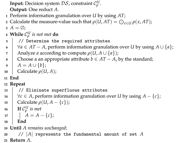
2.4. Strategy Based on Sample

The key of strategy based on sample is compression of sample space [34]. These strategies can immediately reduce the number of scanned samples or comparisons between samples. Here are three classical strategies based on the sample.
  • Bucket based searching for attribute reduction. Liu et al. [10] have considered the bucket method for fast obtaining reduct. A hash function is used in their technique, and every sample in the dataset will then be mapped into a number of separate buckets. Following the intrinsic properties of such a mapping, only samples from the same bucket must be compared rather than samples from the entire dataset. According to this viewpoint, the computing burden of information granulation may be minimized. As a result, the technique for obtaining reduct by the bucket-based strategy is identical to that of Algorithm 1, except for the device of information granulation.
  • Positive approximation for attribute reduction (PAAR). Qian et al. [11] have presented the method based on positive approximation to calculate reduct rapidly. The essence to positive approximation is to compress gradually the sample space. The compressing process should be guided by the values associated with the constrain r h o . The following are the precise steps of the attribute reduction based on positive approximation.
    (1)
    The hypothetical reduct A will be defined as , as well as the sample compressed space U will be defined as U.
    (2)
    By using the constrain of ρ U , A { a } , analyse all hypothetical a A T A which in U .
    (3)
    Using the acquired constrain, choose one qualified attribute b A T A then merge in b to A.
    (4)
    Based on A, calculate ρ U , A and then reanalysis construction of the sample compressed space U .
    (5)
    If the specified constraint is met, produce reduct A; otherwise, back to step(2).
  • Random sampling accelerator for attribute reduction(RSAR). Chen et al. [12] examined the above-mentioned strategies, they found that: (1) Regardless of the searching technique, information granulation over the entire dataset is required; (2) Information granulation over the dataset always needs to be regenerated in each iteration throughout the entire searching process. In this aspect, sample distribution may influence the effectiveness of searching. Therefore, the two above-mentioned strategies have their own restrictions since they are directly tied to sample distribution. The restriction of BBSAR is that Bucket strategy will become inefficient when sample is too centralized, which is time-consuming. The restriction of PAAR is that the sample distribution strongly affect the construction of positive approximation, and then affect the effectiveness of attribute reduction. In view of this, Chen et al. [12] developed a new random sampling strategy. The following shows the exact structure of the random sampling being used to derive reduct.
    (1)
    The samples were randomly separated to n sample groups of equal size: U 1 , , U n .
    (2)
    Compute the reduct A 1 over U 1 ; reduct A 1 will then provide advice for computing the reduct A 2 over U 1 U 2 , and so on.
    (3)
    Get the reduct A n , use it as the ultimate reduct over the entire dataset.
RSAR can reduce the influence of sample distribution on attribute reduction to a certain extent. It is well-known that the reduct obtained from a small volume of samples often does not represent the attribute importance of the entire dataset. However, there are two facts in RSAR: (1) the volume of first sample group is frequently much less than the volume of entire dataset; (2) the reduct obtained from the first sample group is used to guide the reduction calculation of subsequent sample groups which have symmetry. These two facts may reduce the efficiency of attribute reduction. As a result, developing an effective attribute reduction strategy to solve the problem is widely valued.

3. Lift for Attribute Reduction

3.1. Theoretical Foundations

This section provides an attribute reduction strategy based on random sampling and Lift [16] which can select a small volume of represented samples from entire dataset. Lift considers that samples with different labels should have their own characteristics, which should be helpful to find samples with high discernibility.
In Lift, given an n-dimensional attribute space, D L = d 1 , d 2 , , d q represents the finite set of q possible labels possessed by all samples. Therefore, the sample space can be expressed as S = { ( x i , d i ) i = 1 , 2 , , m } , x i is a sample with n-dimensional attribute in the dataset, and d i D L represents the label set of x i . In order to extract the characteristics that can best distinguish one label from every other label, the internal relationship between samples under each label will be consider. Specifically, for a label d k D L , samples are divided into two categories, the positive class samples set P k and the negative class samples set N k , as shown in following:
P k = x i x i , d i S , d k d i ;
N k = x i x i , d i S , d k d i .
For the label d k , if one sample possesses this label, the sample will be classified into positive class, otherwise it will be classified into negative class. In order to explore the internal structures of positive and negative classes, k-means [35] clustering is, respectively, carried out on P k and N k . Since the clustering information of P k can be regarded as equally important with N k , the number of cluster centers is set as m k , that is:
m k = δ · min P k , N k ;
| · | is the cardinality of set; δ [ 0 , 1 ] is the parameters controlling the number of clusters; the cluster centers of P k and N k are recorded as p 1 k , p 2 k , , p m k k and n 1 k , n 2 k , , n m k k .
By utilizing the ability of Lift on selecting the represented samples, we try to give a new strategy for deriving reduct:
(1)
Collect all cluster centers into U 1 .
(2)
The other samples were randomly separated to n − 1 sample groups of equal size: U 2 , , U n .
(3)
Compute the first reduct A 1 over U 1 ; this reduct will then provide advice for computing the second reduct A 2 over U 1 U 2 ; A 2 will also provide advice for computing A 3 over U 1 U 2 U 3 and so on.
(4)
Get the n-th reduct A n , use it as the ultimate reduct over the entire dataset.
According to the previous description, it can be seen that the new strategy provides the following advantages. To begin, when the sample distribution information is unclear, Lift is used to select the most representative samples as the first sample group to better guide the subsequent attribute reduction. Then, except the attribute reduction of the first sample group, the sample distribution will no longer affect the efficiency of attribute reduction of other sample groups which have symmetry. Obviously, these two advantages may aid in reducing the time consumption of attribute reduction.

3.2. Detailed Algorithm

In the worst case of the Algorithm 1, it contains two aspects: (1) There is always only one attribute to be added to the reduct in the each iteration; (2) The final reduct contains all attributes in the dataset. After that, the following will show the time complexity of Algorithm 2.
Remark 1.
The time complexity of Algorithm 2 is O ( 1 n | U | ) 2 · S 1 2 + ( 2 n | U | ) 2 · S 2 2 + + ( n n | U | ) 2 · S n 2 , i.e., O | U | 2 n 2 · i = 1 n ( i 2 · S i 2 ) . For such complexity, n refers to the amount of sample groups, S n indicates the amount attributes ought to be included in the reduct for every iterations, thus i = 1 n S i = S 1 + S 2 + + S n = | A T | . As a result, it is simple to arrive at the following conclusions:
O ( 1 n | U | ) 2 · S 1 2 + ( 2 n | U | ) 2 · S 2 2 + + ( n n | U | ) 2 · S n 2 = O | U | 2 n 2 · i = 1 n ( i 2 · S i 2 ) O | U | 2 n 2 · i = 1 n ( n 2 · S i 2 ) = O | U | 2 · ( i = 1 n S i 2 ) O | U | 2 · ( i = 1 n S i ) 2 ,
i.e., O ( | U | 2 n 2 · i = 1 n ( i 2 · S i 2 ) ) O ( | U | 2 · | A T | 2 ) .
Algorithm 2: Attribute Reduction Based on Lift and Random Sampling
Symmetry 14 01828 i002
In this section, according to the above strategy, an attribute reduction algorithm called ARLRS is proposed as Algorithm 2. In ARLRS, Lift algorithm is used to choose the samples from the dataset as the members of the first group, and random sampling strategy is used to divide the rest of samples into groups. Generally, the reduct of the first sample group is calculated quickly by Algorithm 1. For every subsequent sample group, if the given constrain is satisfied, the attribute reduction calculation of current sample group can be skipped; if the given constrain is not satisfied, the previous sample groups are integrated into the current sample group, then attribute reduction calculation of this integrated group is carried out. As a result, by gradually integrating many previous sample groups, the classification performance of the temporary reduct over the current sample group will be improved until the attribute reduction constrain is met.

4. Analysis of Experiment

4.1. Datasets

To illustrate the effectiveness of the proposed ARLRS algorithm, 17 UCI datasets were chosen for the tests. The UCI datasets is a collection of databases, top level theory, and data generators used by the machine learning to conduct empirical evaluations of machine learning algorithms. David Aha and his fellow graduate students at UC Irvine established the archive as an ftp archive in 1987. Since then, it has been widely used as a key source of machine learning datasets by students, instructors, and researchers all over the world. All the datasets this paper used were download on: https://archive.ics.uci.edu/ml/datasets.php (accessed on 12 January 2022). The Table 1 contains full descriptions of 17 datasets. All experiment were conducted on a personal computer running Windows 10, with an Intel Core i7-6700HQ CPU (2.60 GHz) and 16.00 GB of RAM. Matlab R2019b is the programming language. In order to further analyze the advantages of ARLRS algorithm, the experiment will be shown in two aspects: time consumption and classification performance.

4.2. Basic Experiment Setting

In this paper, the neighborhood rough set [53,54,55,56,57,58] was used as the model for deriving reducts. It should be noted that the computational results of the neighborhood rough set are heavily reliant on the radius chosen, and we pick 0.2 as our radius to illustrate the generality of ARLRS algorithm. Moreover, the concept of approximation quality (Equation (6)) is selected as the constrain of ARLRS algorithm. The approximation quality describes the ability of the approximation in terms of attribute reduction. In general, the higher the degree of approximation quality is, the better performance the selected attribute has.
Five classical algorithms are chosen to compare with the proposed ARLRS algorithm. The four algorithms of them have been introduced detailed in previous context of this paper, that are FGSAR [59,60,61], BBSAR [10], PAAR [11] and RSAR [12]. The fifth compared algorithm is the Attribute Group for Attribute Reduction (AGAR) [62]. AGAR is also a sample based algorithm and has excellent time efficiency and classification performance. Adding AGAR to the comparison can better help us test the performance of ARLRS algorithm.

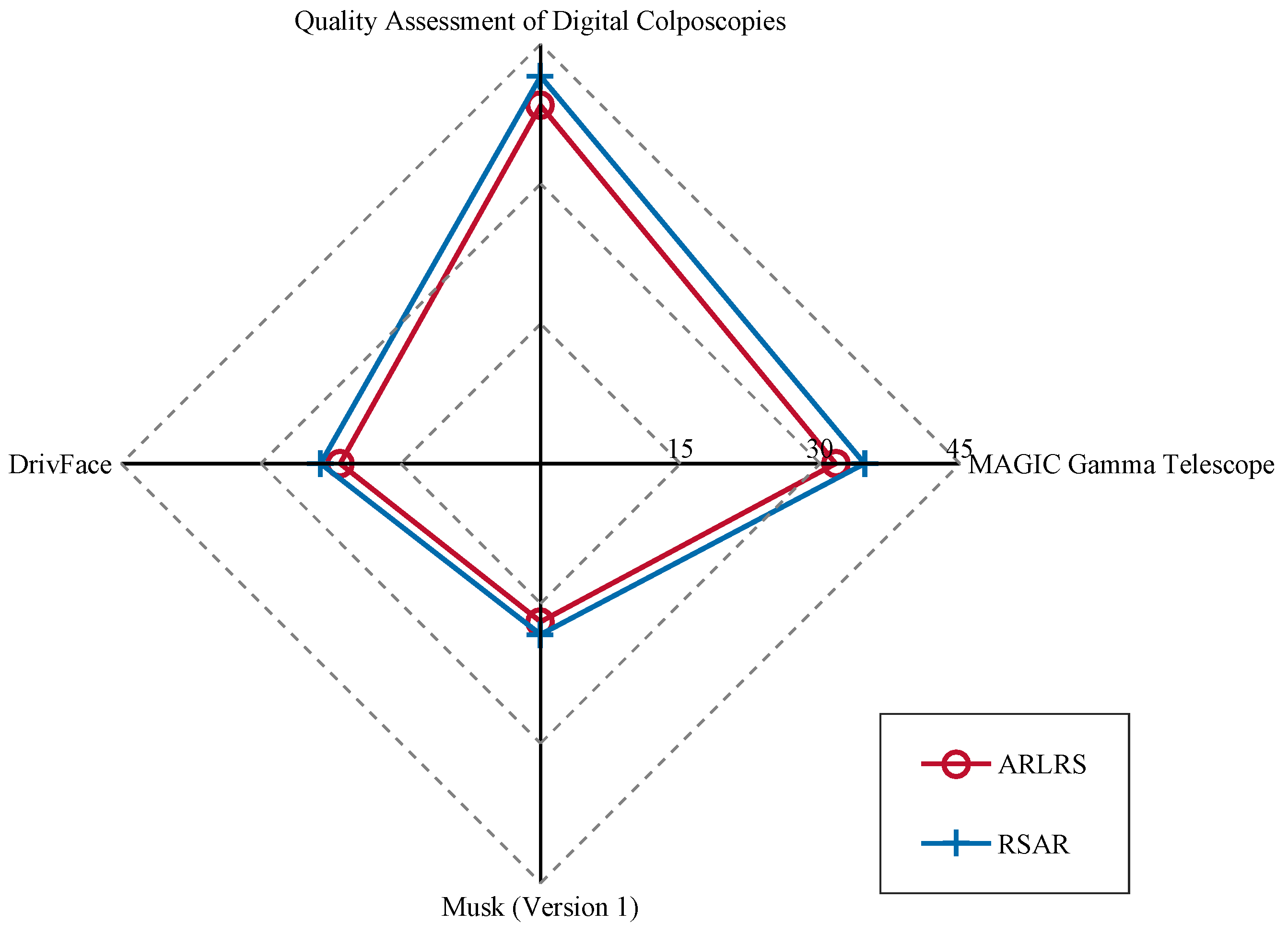
4.3. Time Consumption

In this subsection, the time consumption of five compared algorithms (FGSAR, BBSAR, PAAR, RSAR and AGAR) and ARLRS algorithm on computing reducts are listed in Table 2. For every dataset, the best time consumption is bold.
Table 2 shows that ARLRS performs admirably on time consumption compared to the other five classical algorithms. Using the “QSAR Biodegradation” (ID 13) dataset as an example, the time consumptions of RSAR, FGSAR, PAAR, BBSAR and AGAR are 11.9454, 13.6468, 13.4522, 12.5647 and 12.3949 seconds, respectively. The proposed ARLRS algorithm only takes 9.6467 seconds. Obviously, ARLRS algorithm has the ability to remarkable accelerate the process of computing reduct.
To further demonstrate the superiority of ARLRS algorithm, the speedup ratios of ARLRS algorithm against the five compared algorithms (FGSAR, BBSAR, PAAR, RSAR and AGAR) are shown in Table 3 and the lengths of reducts produced by overall six algorithms are shown in Table 4. It is worth mentioning that FGSAR and PAAR have similar mechanism, so their reduct lengths have symmetry. For every dataset, the shortest length of reducts produced by six algorithms is set bold.
According to Table 3, all speedup ratios of ARLRS algorithm against other five classic sample based algorithms are substantially greater than 1. Even that average speedup ratio approaches 15. These findings show that the proposed ARLRS algorithm can speed up the process of computing reducts from datasets. Furthermore, Table 4 shows that in the most of datasets, the lengths of reducts generated by ARLRS are substantially shorter than those acquired by the other five algorithms. The reducts with shorter length often indicate that ARLRS needs fewer iterations to get the reducts with satisfying classification performance. From this viewpoint, it also shows that ARLRS can effectively reduce the time consumption of attribute reduction.
Among the above six attribute reduction algorithms, ARLRS and RSAR are designed both based on random sampling. It is not difficult to find that for the two algorithms with the similar mechanism, ARLRS algorithm has obvious advantage on the time consumption. Especially on high-dimensional datasets such as “Musk (Version 1)” (ID 14), “DrivFace” (ID 7), “Quality Assessment of Digital Colposcopies” (ID 17) and “MAGIC Gamma Telescope” (ID 11), ARLRS algorithm performs particularly well. In order to better show the advantage of ARLRS algorithm on high-dimensional datasets, Figure 1 shows the time consumption over these four datasets. Obviously, the time consumption of ARLRS is less than that of RSAR over the four high-dimensional datasets.
It is worth mentioning that ARLRS will filter out the samples with low representation, then only evaluate the samples with most representation. The filtration process leads to reduce greatly the time consumption of samples evaluation in the process of attribute reduction. Therefore, comparing with other attribute reduction strategies, the proposed ARLRS algorithm has better performance in time consumption.

4.4. Classification Performance

K-Nearest Neighbor (KNN, K parameter will be set as 3) and Support Vector Machine (SVM) classifiers are used to test the classification accuracies of different reducts produced by six algorithms. The average values of the classification accuracies of generated reducts are provided in Table 5 and Table 6. It is worth mentioning that FGSAR and PAAR have similar mechanism, so the classification performance of them have symmetry. For every dataset, the best classification accuracy is bold.
According to Table 5 and Table 6, ARLRS’s classification performance is somewhat greater than the other five algorithms. Especially for high-dimensional dataset “DrivFace” (ID 7), the classification accuracies of proposed ARLRS are 0.9089 on KNN classifier and 0.8841 on SVM classifier, respectively, which perform better than other five algorithms. As a result, regardless of which two classifiers are utilized, the reducts obtained from ARLRS deliver satisfying classification performance.
It is because Lift can filter out samples with low representation, some candidate attributes will be deleted after the attribute reduction of the first sample group. The subsequent reduction process can receive better guidance for selecting attributes with better classification performance. This mechanism enables the attribute reduction process to focus on attributes with most representation. This is why the classification performances of reducts produced by ARLRS can be satisfying.

4.5. Discussion

In the above experimental analysis, it can be concluded that ARLRS algorithm often performs well in big data, both in terms of time consumption and classification performance, for this conclusion, the following reasons can be given.
(1)
The higher the dimension of the datasets is, the more information the selected sample can carry. Then, the more information can better help to guide the subsequent attribute reduction. Therefore, ARLRS algorithm performs well in handling big data.
(2)
Due to the low value density of big data, it is often necessary to preferentially extract relevant and useful information from a large amount of datasets. The above-mentioned needs are well solved by introducing Lift. The most representative samples found by LIFT make the unclear information under each label have available structure, from the perspective of samples, thus different samples form a certain association. Such preprocessing is very effective in the processing big data, so ARLRS will have certain advantages in processing big data.

5. Conclusions and Future Perspectives

This paper combines Lift with random sampling strategy to proposed an attribute reduction algorithm call ARLRS. The utilization of Lift reduces the impact of overfitting in the first sample group, which can produce the reduct being able to provide better guidance for subsequent attribute reduction. The retainment of random sampling strategy is helpful to reduce the impact of sample distribution. Due to the fact that Lift can mine the samples with most representation, the proposed ARLRS algorithm also has satisfying results in classification performance. The experimental results over 17 UCI datasets show that the above conclusions are effective and credible.
The following research directions will be of great value as our next work.
(1)
In light of the uncertainty existed in constraints and classification performances, the resultant reduct may result in over-fitting. As a result, in future investigation, we will try balance the efficiency of attribute reduction with the classification performance.
(2)
The attribute reduction strategy presented in this research is only applied from the sample’s perspective. Therefore, we will try to investigate some novel algorithms taking into account both samples and attributes for improving more efficiency.

Author Contributions

Conceptualization, T.X.; methodology, T.X.; software, J.C.; validation, T.X.; formal analysis, J.C.; investigation, J.C.; resources, J.C.; data curation, Q.C.; writing—original draft preparation, Q.C.; writing—review and editing, Q.C.; visualization, Q.C.; supervision, T.X.; project administration, T.X. All authors have read and agreed to the published version of the manuscript.

Funding

This work is supported by the National Natural Science Foundation of China (No. 62006099), the Natural Science Foundation of Jiangsu Provincial Colleges and Universities (20KJB520010), and the Key Laboratory of Oceanographic Big Data Mining & Application of Zhejiang Province (No. OBDMA202104).

Institutional Review Board Statement

Not applicable.

Informed Consent Statement

Not applicable.

Data Availability Statement

Not applicable.

Conflicts of Interest

The authors declare no conflict of interest.

References

  1. Chen, D.G.; Yang, Y.Y.; Dong, Z. An incremental algorithm for attribute reduction with variable precision rough sets. Appl. Soft Comput. 2016, 45, 129–149. [Google Scholar] [CrossRef]
  2. Jiang, Z.H.; Yang, X.B.; Yu, H.L.; Liu, D.; Wang, P.X.; Qian, Y.H. Accelerator for multi-granularity attribute reduction. Knowl.-Based Syst. 2019, 177, 145–158. [Google Scholar] [CrossRef]
  3. Ju, H.R.; Yang, X.B.; Yu, H.L.; Li, T.J.; Yu, D.J.; Yang, J.Y. Cost-sensitive rough set approach. Inf. Sci. 2016, 355–356, 282–298. [Google Scholar] [CrossRef]
  4. Qian, Y.H.; Wang, Q.; Cheng, H.H.; Liang, J.Y.; Dang, C.Y. Fuzzy-rough feature selection accelerator. Fuzzy Sets Syst. 2015, 258, 61–78. [Google Scholar] [CrossRef]
  5. Wei, W.; Cui, J.B.; Liang, J.Y.; Wang, J.H. Fuzzy rough approximations for set-valued data. Inf. Sci. 2016, 360, 181–201. [Google Scholar] [CrossRef]
  6. Wei, W.; Wu, X.Y.; Liang, J.Y.; Cui, J.B.; Sun, Y.J. Discernibility matrix based incremental attribute reduction for dynamic data. Knowl.-Based Syst. 2018, 140, 142–157. [Google Scholar] [CrossRef]
  7. Dong, L.J.; Chen, D.G. Incremental attribute reduction with rough set for dynamic datasets with simultaneously increasing samples and attributes. Int. J. Mach. Learn. Cybern. 2020, 11, 213–227. [Google Scholar] [CrossRef]
  8. Zhang, A.; Chen, Y.; Chen, L.; Chen, G.T. On the NP-hardness of scheduling with time restrictions. Discret. Optim. 2017, 28, 54–62. [Google Scholar] [CrossRef]
  9. Guan, L.H. A heuristic algorithm of attribute reduction in incomplete ordered decision systems. J. Intell. Fuzzy Syst. 2019, 36, 3891–3901. [Google Scholar] [CrossRef]
  10. Liu, Y.; Huang, W.L.; Jiang, Y.L.; Zeng, Z.Y. Quick attribute reduct algorithm for neighborhood rough set model. Inf. Sci. 2014, 271, 65–81. [Google Scholar] [CrossRef]
  11. Qian, Y.H.; Liang, J.Y.; Pedrycz, W.; Dang, C.Y. Positive approximation: An accelerator for attribute reduction in rough set theory. Artif. Intell. 2010, 174, 597–618. [Google Scholar] [CrossRef]
  12. Chen, Z.; Liu, K.Y.; Yang, X.B.; Fujita, H. Random sampling accelerator for attribute reduction. Int. J. Approx. Reason. 2022, 140, 75–91. [Google Scholar] [CrossRef]
  13. Wang, K.; Thrampoulidis, C. Binary classification of gaussian mixtures: Abundance of support vectors, benign overfitting, and regularization. SIAM J. Math. Data Sci. 2022, 4, 260–284. [Google Scholar] [CrossRef]
  14. Bejani, M.M.; Ghatee, M.A. A systematic review on overfitting control in shallow and deep neural networks. Artif. Intell. Rev. 2021, 54, 6391–6438. [Google Scholar] [CrossRef]
  15. Park, Y.; Ho, J.C. Tackling overfitting in boosting for noisy healthcare data. IEEE Trans. Knowl. Data Eng. 2021, 33, 2995–3006. [Google Scholar] [CrossRef]
  16. Zhang, M.L.; Wu, L. Lift: Multi-label learning with label-specific features. IEEE Trans. Pattern Anal. Mach. Intell. 2015, 37, 107–120. [Google Scholar] [CrossRef] [PubMed]
  17. Hu, Q.H.; Zhang, L.; Chen, D.G.; Pedrycz, W.; Yu, D. Gaussian kernel based fuzzy rough sets: Model, uncertainty measures and applications. Int. J. Approx. Reason. 2010, 51, 453–471. [Google Scholar] [CrossRef]
  18. Sun, L.; Wang, L.Y.; Ding, W.P.; Qian, Y.H.; Xu, J.C. Feature selection using fuzzy neighborhood entropy-nased uncertainty measures for fuzzy neighborhoodm mltigranulation rough sets. IEEE Trans. Fuzzy Syst. 2021, 29, 19–33. [Google Scholar] [CrossRef]
  19. Wang, Z.C.; Hu, Q.H.; Qian, Y.H.; Chen, D.E. Label enhancement-based feature selection via fuzzy neighborhood discrimination index. Knowl.-Based Syst. 2022, 250, 109119. [Google Scholar] [CrossRef]
  20. Li, W.T.; Wei, Y.L.; Xu, W.H. General expression of knowledge granularity based on a fuzzy relation matrix. Fuzzy Sets Syst. 2022, 440, 149–163. [Google Scholar] [CrossRef]
  21. Liu, F.L.; Zhang, B.W.; Ciucci, D.; Wu, W.Z.; Min, F. A comparison study of similarity measures for covering-based neighborhood classifiers. Inf. Sci. 2018, 448–449, 1–17. [Google Scholar] [CrossRef]
  22. Ma, X.A.; Yao, Y.Y. Min-max attribute-object bireducts: On unifying models of reducts in rough set theory. Inf. Sci. 2019, 501, 68–83. [Google Scholar] [CrossRef]
  23. Xu, T.H.; Wang, G.Y.; Yang, J. Finding strongly connected components of simple digraphs based on granulation strategy. Int. J. Approx. Reason. 2020, 118, 64–78. [Google Scholar] [CrossRef]
  24. Jia, X.Y.; Rao, Y.; Shang, L.; Li, T.J. Similarity-based attribute reduction in rough set theory: A clustering perspective. Int. J. Approx. Reason. 2020, 11, 1047–1060. [Google Scholar] [CrossRef]
  25. Ding, W.P.; Pedrycz, W.; Triguero, I.; Cao, Z.H.; Lin, C.T. Multigranulation supertrust model for attribute reduction. IEEE Trans. Fuzzy Syst. 2021, 29, 1395–1408. [Google Scholar] [CrossRef]
  26. Chu, X.L.; Sun, B.D.; Chu, X.D.; Wu, J.Q.; Han, K.Y.; Zhang, Y.; Huang, Q.C. Multi-granularity gominance rough concept attribute reduction over hybrid information systems and its application in clinical decision-making. Inf. Sci. 2022, 597, 274–299. [Google Scholar] [CrossRef]
  27. Yuan, Z.; Chen, H.M.; Yang, X.L.; Li, T.R.; Liu, K.Y. Fuzzy complementary entropy using hybrid-kernel function and its unsupervised attribute reduction. Knowl.-Based Syst. 2021, 231, 107398. [Google Scholar] [CrossRef]
  28. Zhang, Q.Y.; Chen, Y.; Zhang, G.Q.; Li, Z.; Chen, L.; Wen, C.F. New uncertainty measurement for categorical data based on fuzzy information structures: An application in attribute reduction. Inf. Sci. 2021, 580, 541–577. [Google Scholar] [CrossRef]
  29. Ding, W.P.; Wang, J.D.; Wang, J.H. Multigranulation consensus fuzzy-rough based attribute reduction. Knowl.-Based Syst. 2020, 198, 105945. [Google Scholar] [CrossRef]
  30. Chen, Y.; Yang, X.B.; Li, J.H.; Wang, P.X.; Qian, Y.H. Fusing attribute reduction accelerators. Inf. Sci. 2022, 587, 354–370. [Google Scholar] [CrossRef]
  31. Yan, W.W.; Ba, J.; Xu, T.H.; Yu, H.L.; Shi, J.L.; Han, B. Beam-influenced attribute selector for producing stable reduct. Mathematics 2022, 10, 533. [Google Scholar] [CrossRef]
  32. Ganguly, S.; Bhowal, P.; Oliva, D.; Sarkar, R. BLeafNet: A bonferroni mean operator based fusion of CNN models for plant identification using leaf image classification. Ecol. Inform. 2022, 69, 101585. [Google Scholar] [CrossRef]
  33. Zhang, C.F.; Feng, Z.L. Convolutional analysis operator learning for multifocus image fusion. Signal Process. Image Commun. 2022, 103, 116632. [Google Scholar] [CrossRef]
  34. Jiang, Z.H.; Dou, H.L.; Song, J.J.; Wang, P.X.; Yang, X.B.; Qian, Y.H. Data-guided multi-granularity selector for attribute eduction. Artif. Intell. Rev. 2021, 51, 876–888. [Google Scholar] [CrossRef]
  35. Kanungo, T.; Mount, D.M.; Netanyahu, N.S.; Piatko, C.D.; Silverman, R.; Wu, A.Y. An efficient k-means clustering algorithm: Analysis and implementation. IEEE Trans. Pattern Anal. Mach. Intell. 2002, 24, 881–892. [Google Scholar] [CrossRef]
  36. Quinlan, J.R. Simplifying decision trees. Int. J.-Hum.-Comput. Stud. 1999, 51, 497–510. [Google Scholar] [CrossRef]
  37. Street, N.; Wolberg, W.; Mangasarian, O. Nuclear feature extraction for breast tumor diagnosis. Int. Symp. Electron. Imaging Sci. Technol. 1999, 1993, 861–870. [Google Scholar] [CrossRef]
  38. Ayres-de-Campos, D.; Bernardes, J.; Garrido, A.; Marques-de-sá, J.; Pereira-leite, L. SisPorto 2.0: A program for automated analysis of cardiotocograms. J. Matern.-Fetal Med. 2000, 9, 311–318. [Google Scholar] [CrossRef]
  39. Gorman, R.P.; Sejnowski, T.J. Analysis of hidden units in a layered network trained to classify sonar sargets. Neural Netw. 1988, 16, 75–89. [Google Scholar] [CrossRef]
  40. Johnson, B.A.; Iizuka, K. Integrating open street map crowd sourced data and landsat time-series imagery for rapid land use/land cover (LULC) mapping: Case study of the laguna de bay area of the philippines. Appl. Geogr. 2016, 67, 140–149. [Google Scholar] [CrossRef]
  41. Antal, B.; Hajdu, A. An ensemble-based system for automatic screening of diabetic retinopathy. Knowl.-Based Syst. 2014, 60, 20–27. [Google Scholar] [CrossRef]
  42. Díaz-Chito, K.; Hernàndez, A.; López, A. A reduced feature set for driver head pose estimation. Appl. Soft Comput. 2016, 45, 98–107. [Google Scholar] [CrossRef]
  43. Johnson, B.; Tateishi, R.; Xie, Z. Using geographically-weighted variables for image classification. Remote Sens. Lett. 2012, 3, 491–499. [Google Scholar] [CrossRef]
  44. Evett, I.W.; Spiehler, E.J. Rule induction in forensic science. Knowl. Based Syst. 1989, 152–160. Available online: https://dl.acm.org/doi/abs/10.5555/67040.67055 (accessed on 15 August 2022).
  45. Sigillito, V.; Wing, S.; Hutton, L.; Baker, K. Classification of radar returns from the ionosphere using neural networks. Johns Hopkins APL Tech. Dig. 1989, 10, 876–890. [Google Scholar] [CrossRef]
  46. Bock, R.K.; Chilingarian, A.; Gaug, M.; Hakl, F.; Hengstebeck, T.; Jiřina, M.; Klaschka, J.; Kotrč, E.; Savický, P.; Towers, S.; et al. Methods for multidimensional event classification: A case study using images from a cherenkov gamma-ray telescope. Nucl. Instrum. Methods Phys. Res. Sect. Accel. Spectrometers Detect. Assoc. Equip. 2004, 516, 511–528. [Google Scholar] [CrossRef]
  47. Sakar, B.E.; Isenkul, M.E.; Sakar, C.O.; Sertbas, A.; Gurgen, F.; Delil, S.; Apaydin, H.; Kursun, O. Collection and analysis of a parkinson speech dataset with multiple types of sound recordings. IEEE J. Biomed. Health Inform. 2013, 17, 828–834. [Google Scholar] [CrossRef]
  48. Mansouri, K.; Ringsted, T.; Ballabio, D.; Todeschini, R.; Consonni, V. Quantitative structure–activity relationship models for ready biodegradability of chemicals. J. Chem. Inf. Model. 2013, 53, 867–878. [Google Scholar] [CrossRef]
  49. Dietterich, T.G.; Lathrop, R.H.; Lozano-Pérez, T. Solving the multiple instance problem with axis-parallel rectangles. Artif. Intell. 1997, 89, 31–71. [Google Scholar] [CrossRef]
  50. Malerba, D.; Esposito, F.; Semeraro, G. A further comparison of simplification methods for decision-tree induction. In Learning from Data; Springer: New York, NY, USA, 1996; pp. 365–374. [Google Scholar] [CrossRef]
  51. Johnson, B.; Xie, Z. Classifying a high resolution image of an urban area using super-object information. ISPRS J. Photogramm. Remote Sens. 2013, 83, 40–49. [Google Scholar] [CrossRef]
  52. Fernandes, K.; Cardoso, J.S.; Fernandes, J. Transfer learning with partial observability applied to cervical cancer screening. Pattern Recognit. Image Anal. 2017, 243–250. [Google Scholar] [CrossRef]
  53. Sun, L.; Wang, T.X.; Ding, W.P.; Xu, J.C.; Lin, Y.J. Feature selection using fisher score and multilabel neighborhood rough sets for multilabel classification. Inf. Sci. 2021, 578, 887–912. [Google Scholar] [CrossRef]
  54. Luo, S.; Miao, D.Q.; Zhang, Z.F.; Zhang, Y.J.; Hu, S.D. A neighborhood rough set model with nominal metric embedding. Inf. Sci. 2020, 520, 373–388. [Google Scholar] [CrossRef]
  55. Chu, X.L.; Sun, B.Z.; Li, X.; Han, K.Y.; Wu, J.Q.; Zhang, Y.; Huang, Q.C. Neighborhood rough set-based three-way clustering considering attribute correlations: An approach to classification of potential gout groups. Inf. Sci. 2020, 535, 28–41. [Google Scholar] [CrossRef]
  56. Shu, W.H.; Qian, W.B.; Xie, Y.H. Incremental feature selection for dynamic hybrid data using neighborhood rough set. Knowl.-Based Syst. 2020, 194, 105516. [Google Scholar] [CrossRef]
  57. Wan, J.H.; Chen, H.M.; Yuan, Z.; Li, T.R.; Sang, B.B. A novel hybrid feature selection method considering feature interaction in neighborhood rough set. Knowl.-Based Syst. 2021, 227, 107167. [Google Scholar] [CrossRef]
  58. Sang, B.B.; Chen, H.M.; Yang, L.; Li, T.R.; Xu, W.H.; Luo, W.H. Feature selection for dynamic interval-valued ordered data based on fuzzy dominance neighborhood rough set. Knowl.-Based Syst. 2021, 227, 107223. [Google Scholar] [CrossRef]
  59. Hu, Q.H.; Xie, Z.X.; Yu, D. Hybrid attribute reduction based on a novel fuzzy-rough model and information granulation. Pattern Recognit. 2007, 40, 3509–3521. [Google Scholar] [CrossRef]
  60. Jensen, R.; Qiang, S. Fuzzy–rough attribute reduction with application to web categorization. Fuzzy Sets Syst. 2004, 141, 469–485. [Google Scholar] [CrossRef]
  61. Xu, S.P.; Yang, X.B.; Yu, H.L.; Yu, D.J.; Yang, J.Y.; Tsang, E.C. Multi-label learning with label-specific feature reduction. Knowl.-Based Syst. 2016, 104, 52–61. [Google Scholar] [CrossRef]
  62. Chen, Y.; Liu, K.Y.; Song, J.J.; Yang, X.B.; Qian, Y.H. Attribute group for attribute reduction. Inf. Sci. 2020, 535, 64–80. [Google Scholar] [CrossRef]
Figure 1. Time consumption of attribute reduction on high-dimensional datasets.
Symmetry 14 01828 g001
Table 1. Datasets used in the experiment.
IDDatasets# Samples# Attributes# LabelsAttributes Type
1Australian Credit Approval [36]690142Real
2Breast Cancer Wisconsin (Diagnostic) [37]569302Real
3Cardiotocography [38]21262110Real
4Connectionist Bench (Sonar, Mines vs. Rocks) [39]208602Real
5Crowdsourced Mapping [40]10,845286Real
6Diabetic Retinopathy Debrecen [41]1151192Integer & Real
7DrivFace [42]60664003Real
8Forest Type Mapping [43]523274Integer & Real
9Glass Identification [44]21496Real
10Ionosphere [45]351342Integer & Real
11MAGIC Gamma Telescope [46]19,020286Real
12Parkinson Multiple Sound Recording [47]1208262Real
13QSAR Biodegradation [48]1055412Real
14Musk (Version 1) [49]4761662Integer
15Page Blocks Classification [50]5473105Integer & Real
16Urban Land Cover [51]6751479Integer & Real
17Quality Assessment of Digital Colposcopies [52]287622Real
Table 2. The time consumption (unit is second) of six attribute reduction algorithms.
IDARLRSRSARFGSARPAARBBSARAGAR
11.34391.60461.96831.95333.03782.0001
22.85143.26163.75533.64744.98786.3496
31.71562.37403.62153.34524.02482.6923
43.1143.87124.65344.45324.94586.3526
50.03310.03510.35610.34240.41380.0493
61.50431.65423.34623.39772.77453.4527
721.507121.607422.954322.646432.744124.2342
83.27074.917310.273210.24804.42534.5429
936.682539.917355.452454.280946.35540.6939
102.21562.37403.56433.57544.02482.5551
1132.654234.764535.347535.334235.457834.9578
122.51272.75453.16423.00082.83613.147
139.646711.945413.646813.452212.564712.3949
1416.965518.336119.746819.231219.148518.5435
1544.455446.126548.464148.852945.565948.4844
163.61254.04154.83534.12374.72644.9645
1738.412441.541543.851543.452945.455444.5455
Table 3. The speed up ratio of five compared algorithms to ARLRS.
IDRSARFGSARPAARBBSARAGAR
116.3731.1941.1730.3432.81
212.5824.0721.8220.5319.31
327.7335.1227.8218.2126.34
419.6333.1430.1325.757.22
52.3623.382.652.7117.78
69.0614.6442.9134.5227.98
713.1519.0118.624.575.99
88.1133.8532.4234.919.86
920.1337.8438.0324.2413.29
1010.2311.0922.9723.1330.23
116.077.027.887.916.59
1225.9720.5916.2711.4020.16
1319.249.397.7123.2222.17
1425.0918.2813.7112.936.77
153.628.276.002.448.31
1615.2313.8814.7617.8420.76
1731.254.336.127.3215.9
avg15.6320.2920.6417.7917.14
Table 4. Reduct lengths of six algorithms.
IDARLRSRSARFGSARPAARBBSARAGAR
17.147.328.038.038.037.17
28.678.219.199.199.198.11
37.388.667.577.577.578.45
47.137.438.178.178.177.43
514.3415.3214.3814.3814.3816.64
69.469.218.328.328.328.76
78.749.877.157.157.159.75
88.659.079.259.259.258.98
97.919.878.578.578.578.07
108.658.978.788.788.789.21
1123.8724.5825.3225.3225.3227.98
127.0310.3410.0110.0110.019.28
136.989.018.348.348.347.32
148.758.658.908.908.9010.76
1513.6615.3216.2416.2416.2415.23
1614.3115.0915.6515.6515.6516.32
178.028.068.198.198.199.15
Table 5. Based on KNN classifier, the classification accuracies of reducts produced by six attribute reduction algorithms.
IDARLRSRSARFGSARPAARBBSARAGAR
10.85550.87420.81680.81680.85570.9175
20.97850.90000.85340.85340.93470.9456
30.93990.93200.88240.88240.83560.8943
40.95690.96420.80740.80740.97410.9456
50.88480.83510.80220.80220.81490.8624
60.84490.82720.90740.90740.87360.8488
70.90890.90030.80750.80750.85720.8197
80.84370.83260.87310.87310.81860.8279
90.84410.87410.85070.85070.91170.7986
100.95750.93200.92690.92690.83560.8943
110.91450.84870.83660.83660.88690.8747
120.90350.90550.92660.92660.88450.8647
130.83640.86410.86440.86440.91530.8279
140.96340.95340.91280.91280.89340.8634
150.93140.91690.86740.86740.84670.8469
160.92990.90640.87960.87960.90740.8534
170.80360.87120.86420.86420.85410.8779
Table 6. Based on SVM classifier, the classification accuracies of reducts produced by six attribute reduction algorithms.
IDARLRSRSARFGSARPAARBBSARAGAR
10.83960.86140.83180.83180.84960.8779
20.89840.84010.83020.83020.71210.7326
30.83510.87410.91640.91640.88130.8801
40.84330.83810.80410.80410.87010.8912
50.91030.87010.93280.93280.94880.8468
60.94340.93620.97230.97230.93560.9147
70.88410.87660.84520.84520.81410.7998
80.83210.83110.97230.97230.73180.7323
90.91940.92480.90490.90490.87220.8413
100.89540.88880.77630.77630.80520.7113
110.91650.89710.94600.94600.87410.8492
120.93650.92070.91940.91940.82790.7812
130.91530.88030.74360.74360.77990.8940
140.89150.87660.86220.86220.83480.8786
150.92550.89030.88020.88020.85840.9205
160.90440.89090.86330.86330.82610.8759
170.87590.92040.88160.88160.93620.8294
Publisher’s Note: MDPI stays neutral with regard to jurisdictional claims in published maps and institutional affiliations.

