Global Stability of a Second-Order Exponential-Type Difference Equation

Abstract

In this work, we explore the boundedness and local and global asymptotic behavior of the solutions to a second-order difference formula of the exponential type ${\xi }_{n+1}=a+b{\xi }_{n-1}+c{\xi }_{n-1}{e}^{-\rho {\xi }_n}$, where $a,c,\rho \in (0,\infty )$, $b\in (0,1)$ and the initials ${\xi }_0,{\xi }_{-1}$ are non-negative real numbers. Some other special cases are given. We provide two concrete numerical examples to confirm the theoretical results.

1. Introduction and Preliminaries

The study of non-linear difference formulas has sparked a lot of attention recently. The research of non-linear difference formulas brings considerable difficulty to mathematicians and is also extremely gratifying because of its great applications in various fields of applied as well as pure mathematics. This type of equation arises from probability theory, psychology, biology, population, genetics, economics, etc. For some papers in this direction, we refer to [1,2,3,4,5].

Exponential-type difference equations are among the most essential sorts of non-linear difference formulas. H. El-metwally et al. [6] examined the global stability of

$${\xi }_{n+1}=c+d{\xi }_{n-1}{e}^{-{\xi }_n},$$

where $c,d$ and the initials ${\xi }_0,{\xi }_1$ are positive real numbers. This formula might check out as a model, where c is the migration rate, and d is the population growth rate.

In [7], the global asymptotic stability of

$${\xi }_{n+1}=\frac{a+b{e}^{-{\xi }_n}}{c+{\xi }_{n-1}},$$

$n=0,1,2,\dots$ is investigated where $a,c$, and b are positive numbers.

Ding et al. [8] studied a discrete population equation in the form

$${\xi }_{n+1}=(a{\xi }_n+b{\xi }_{n-1})e^{-{\xi }_n},$$

where ${\xi }_0,{\xi }_1>0$, $n=1,2,\dots$, $a\in (0,1)$, $b\in (0,\infty )$.

The purpose of our work is to study the local behavior, boundedness, and behavior of difference formula in the exponential type

$${\xi }_{n+1}=a+b{\xi }_{n-1}+c{\xi }_{n-1}{e}^{-\rho {\xi }_n},$$

(1)

where $a,c,\rho \in (0,\infty )$, $b\in (0,1)$ and the initials ${\xi }_0,{\xi }_{-1}$ are positive real numbers.

For even more results of the exponential-type difference formulas and related results, we refer the reader to [9,10,11,12,13,14,15,16,17].

For some outcomes of the systems of exponential-type difference formulas, we can see [1,18,19].

Let J be an interval in $\mathbb{R}$ and $h:J\times J\to J$ be a continuous function.

Consider

$${\xi }_{n+1}=h({\xi }_n,{\xi }_{n-1}),n=0,1,2\dots$$

(2)

where the initials ${\xi }_0,{\xi }_{-1}\in J$.

The linearized equation in Equation (2) about the equilibrium $\tilde{\xi }$ is

$${\eta }_{n+1}=s{\eta }_n+t{\eta }_{n-1},n=0,1,2\dots ,$$

(3)

where $s=\frac{\partial h}{\partial \xi }(\tilde{\xi },\tilde{\xi })$, $t=\frac{\partial h}{\partial \eta }(\tilde{\xi },\tilde{\xi })$ are the partial derivatives of $h(\xi ,\eta )$ at $\tilde{\xi }$ of Equation (2).

The characteristic equation in Equation (3) is the equation

$${\lambda }^2-s\lambda -t=0,$$

(4)

with the characteristic roots

$${\lambda }_1,{\lambda }_2=\frac{s\pm \sqrt{s^2+4t}}{2}.$$

The following theorem is an essential tool to determine the local asymptotic stability of $\tilde{\xi }$.

Theorem 1

(Linearized stability theorem) (see [14]).

(i) 

The equilibrium $\tilde{\xi }$ of Equation (2) is locally asymptotically stable if both solutions to Equation (4) have absolute values less than one.

(ii) 

A sufficient and necessary condition for both roots of Equation (4) to have an absolute value less than one is

$$\left|s\right|<1-t<2.$$

(iii) 

$\tilde{\xi }$ of Equation (2) is unstable if at least one of the solutions to Equation (4) has an absolute value greater than one.

(iv) 

A sufficient and necessary condition for one root of Equation (4) to have an absolute value less than one and the other root of Equation (4) to have an absolute value greater than one is

$$s^2>-4t,\left|s\right|>|1-t|.$$

So, $\tilde{\xi }$ is called a saddle-point equilibrium.

Theorem 2

(A comparison theorem) (see [20]). Let $a\in (0,\infty )$ and $b\in \mathbb{R}$. Let ${\left\{{\xi }_n\right\}}_{n=-1}^{\infty }$ and ${\left\{{\eta }_n\right\}}_{n=-1}^{\infty }$ be sequences in $\mathbb{R}$ provided that ${\xi }_0<{\eta }_0$, ${\xi }_{-1}<{\eta }_{-1}$ and ${\xi }_{n+1}\le s{\xi }_{n-1}+t$,${\eta }_{n+1}=s{\eta }_{n-1}+t$. Then, ${\xi }_n<{\eta }_n$ for $n\ge -1$.

The following important theorem is the primary tool to study the convergence of solutions to Equation (2).

Theorem 3

(see [14]). Suppose:

(i) 

There are positive numbers s and t with $s\le t$ such that $s\le f(\xi ,\eta )\le t$ for all $\xi ,\eta \in [s,t]$.

(ii) 

$f(\xi ,\eta )$ is decreasing in $\xi \in [s,t]$ for each $\eta \in [s,t]$, and $f(\xi ,\eta )$ is increasing in $\eta \in [s,t]$ for each $\xi \in [s,t]$.

(iii) 

Equation (2) has no solutions for the second prime period in $[s,t]$.

Then, there is one equilibrium $\tilde{\xi }$ of Equation (2) that lies in $[s,t]$. Moreover, every solution to Equation (2) with the initials ${\xi }_0,{\xi }_{-1}\in [s,t]$ converges to $\tilde{\xi }$.

2. Local Asymptotic Stability Analysis

In this section, we study the existence of a unique equilibrium $\tilde{\xi }$ and the local asymptotic stability of solutions.

The equilibriums of Equation (1) are the solutions to

$$\tilde{\xi }=a+b\tilde{\xi }+c\tilde{\xi }{e}^{-\rho \tilde{\xi }}.$$

(5)

Set

$$g(\xi )=a+\{b+c{e}^{-\rho \xi }-1\}\xi .$$

Then, $g(0)=a$, and ${lim}_{x\to \infty }g(\xi )=-\infty$.

Moreover,

$$g^{\prime }(\xi )=b+c{e}^{-\rho \xi }-1-c\rho \xi e^{-\rho \xi }=(b-1)+c(1-\rho \xi )e^{-\rho \xi }.$$

This means that Equation (5) has exactly one solution $\tilde{\xi }$, and, furthermore, $\tilde{\xi }>\frac{a}{-b+1}$.

Theorem 4.

Suppose that

$$c<(-b+1)\{\frac{-a+\sqrt{a^2+\frac{4a(-b+1)}{\rho }}}{a+\sqrt{a^2+\frac{4a(-b+1)}{\rho }}}{e}^{\frac{\rho \{a+\sqrt{a^2+\frac{4a(-b+1)}{\rho }}\}}{2(-b+1)}}\}.$$

(6)

Then, $\tilde{\xi }$ of Equation (1) is locally asymptotically stable.

Proof. 

The linearized equation of Equation (1) about $\tilde{\xi }$ is

$$S_{n+1}-\rho (a+(b-1)\tilde{\xi })S_n-(1-\frac{a}{\tilde{\xi }})S_{n-1}=0.$$

The characteristic equation is

$${\lambda }^2-\rho (a+(b-1)\tilde{\xi })\lambda -(1-\frac{a}{\tilde{\xi }})=0.$$

By using Theorem 1, we see that $\tilde{\xi }$ is locally asymptotically stable if

$$\tilde{\xi }<\frac{a+\sqrt{a^2+\frac{4a(-b+1)}{\rho }}}{2(-b+1)}.$$

(7)

From (5) and Inequality (7), we can obtain Inequality (6).  □

Corollary 1.

If

$$(-b+1)\{\frac{\sqrt{a^2+\frac{4a(-b+1)}{\rho }}-a}{\sqrt{a^2+\frac{4a(-b+1)}{\rho }}+a}{e}^{\frac{\rho \{a+\sqrt{a^2+\frac{4a(-b+1)}{\rho }}\}}{2(-b+1)}}\}<c,$$

then $\tilde{\xi }$ is unstable.

Remark 1.

We note that $\tilde{\xi }$ is a saddle point.

3. Boundedness of Solutions

We establish a suitable condition for the boundedness of solutions.

Theorem 5.

Every positive solution of Equation (1) is bounded if

$$c<(-b+1)e^{\frac{\rho a}{(-b+1)}}.$$

(8)

Proof. 

Let ${\left\{{\xi }_n\right\}}_{n=-1}^{\infty }$ be a solution to Equation (1). For all $n\ge 1$,

$${\xi }_{n+1}=a+b{\xi }_{n-1}+c{\xi }_{n-1}{e}^{-\rho {\xi }_n}<a+b{\xi }_{n-1}+c{\xi }_{n-1}{e}^{\frac{\rho a}{b-1}}.$$

Now, we consider the equation

$${\eta }_{n+1}=a+\eta {\eta }_{n-1},\eta =b+c{e}^{\frac{\rho a}{b-1}}.$$

(9)

The solution ${\left\{{\eta }_n\right\}}_{n=-1}^{\infty }$ of Equation (9) is given by

$${\eta }_n=\frac{a}{1-\eta }+r_1{(\eta )}^{n/2}+r_2{(-\eta )}^{n/2},$$

(10)

where $r_1$ and $r_2$ depend on the initials ${\eta }_0$ and ${\eta }_{-1}$. Thus, Equations (8) and (10) imply that ${\eta }_n$ is a bounded sequence. Now, we shall consider ${\eta }_n$ of Equation (9) such that ${\eta }_0={\xi }_0$ and ${\eta }_1={\xi }_1$. By Theorem 2, we have ${\xi }_n<{\eta }_n$, $n\ge 1$. So, ${\xi }_n$ is bounded.  □

Corollary 2.

Equation (1) has positive unbounded solutions if

$$c<(-b+1)e^{\frac{\rho a}{(-b+1)}}.$$

4. Global Asymptotic Stability Analysis

We derive the suitable condition in which the $\tilde{\xi }$ of Equation (1) is globally asymptotically stable.

Theorem 6.

Consider Equation (1) such that the initials ${\xi }_0,{\xi }_{-1}$ are positive constants and

$$c<\{\frac{-\rho a+\sqrt{{(\rho a)}^2+4{(-b+1)}^4}}{2(-b+1)}\}{e}^{\frac{\rho a}{-b+1}}.$$

(11)

Then, Equation (1) has no positive solution for the second prime period.

Proof. 

Let $\xi ,\eta \in (a,\infty )$ with

$$\xi =a+b\xi +c\xi e^{-\rho \eta },\eta =a+b\eta +c\eta e^{-\rho \xi }.$$

We will show that $\xi =\eta$.

Now, we note that

$$\eta =-\frac{1}{\rho }ln[\frac{(-b+1)\xi -a}{c\xi }],$$

and

$$\xi =-\frac{1}{\rho }ln[\frac{(-b+1)\eta -a}{c\eta }].$$

So,

$$(-b+1-c{e}^{-\rho \xi })(\frac{-1}{\rho })ln[\frac{(-b+1)\xi -a}{c\xi }]=\frac{a}{-b+1}$$

$$=(-b+1-c{e}^{-\rho \eta })(\frac{-1}{\rho })ln[\frac{(-b+1)\eta -a}{c\eta }].$$

Set

$$F(z)=(\frac{-1}{\rho })(-b+1-c{e}^{-\rho z})ln[\frac{(-b+1)z-a}{cz}]-\frac{a}{-b+1}.$$

Clearly, $F(\tilde{\xi })=0$. We will show $F(z)$ has exactly one z-intercept greater than $\frac{a}{-b+1}$.

Let $z>\frac{a}{-b+1}$ be such that $F(z)=0$. We shall try to show that $F^{\prime }(z)<0$. Now,

$$F^{\prime }(z)=(\frac{-1}{\rho })\{\frac{(-b+1-c{e}^{-\rho z})a}{z((-b+1)z-a)}\}+\rho c{e}^{-\rho z}ln[\frac{(-b+1)z-a}{cz}].$$

As $F(z)=0$, we have

$$ln[\frac{(-b+1)z-a}{cz}]=\frac{-\rho a}{(-b+1)(-b+1-c{e}^{-\rho z})}.$$

So,

$$F^{\prime }(z)=(\frac{-1}{\rho })\{\frac{a(-b+1-c{e}^{-\rho z})}{z((-b+1)z-a)}-\frac{{\rho }^{2}ac{e}^{-\rho z}}{(-b+1)(-b+1-c{e}^{-\rho z})}\}$$

$$=\frac{-a(-b+1-c{e}^{-\rho z})}{\rho z((-b+1)z-a)}+\frac{\rho ac{e}^{-\rho z}}{(-b+1)(-b+1-c{e}^{-\rho z})}.$$

$F^{\prime }(z)<0$ if and only if

$${\rho }^{2}cz((-b+1)z-a)<(-b+1){(-b+1-c{e}^{-\rho z})}^2{e}^{\rho z}.$$

For $z>\frac{a}{-b+1}$, set

$$g(z)=(-b+1){(-b+1-c{e}^{-\rho z})}^2{e}^{\rho z}$$

and

$$h(z)={\rho }^{2}cz((-b+1)z-a).$$

Now,

$$g(\frac{a}{-b+1})-h(\frac{a}{-b+1})=(-b+1){(-b+1-c{e}^{\frac{-\rho a}{-b+1}})}^2{e}^{\frac{\rho a}{-b+1}}>0.$$

Moreover,

$$g^{\prime }(z)=(-b+1)\{{(-b+1-c{e}^{-\rho z})}^2\rho e^{\rho z}+2e^{\rho z}(-b+1-c{e}^{-\rho z})(c\rho e^{-\rho z})\}$$

$$=\rho (-b+1)(-b+1-c{e}^{-\rho z})e^{\rho z}\{(-b+1-c{e}^{-\rho z})+zc{e}^{-\rho z}\}$$

$$=\rho (-b+1)e^{\rho z}\{{(-b+1)}^2-c^2{e}^{-2\rho z}\}.$$

$$h^{\prime }(z)={\rho }^{2}c\{2(-b+1)z-a\}.$$

$$g^{\prime }(\frac{a}{-b+1})-h^{\prime }(\frac{a}{-b+1})=\rho (-b+1)e^{\frac{\rho a}{-b+1}}\{{(-b+1)}^2-c^2{e}^{\frac{-2\rho a}{-b+1}}\}-{\rho }^{2}ca.$$

By using Inequality (11), we have $g^{\prime }(\frac{a}{-b+1})-h^{\prime }(\frac{a}{-b+1})>0$.

Now,

$$g^{″}(z)={\rho }^2(-b+1)e^{\rho z}\{c^2{e}^{-2\rho z}+{(-b+1)}^2\}={\rho }^2(-b+1)e^{\rho z}\{{(c{e}^{-\rho z})}^2+{(-b+1)}^2\}.$$

$$h^{″}(z)=2{\rho }^{2}c(-b+1).$$

$$g^{″}(\frac{a}{-b+1})-h^{″}(\frac{a}{-b+1})={\rho }^2(-b+1)e^{\frac{\rho a}{-b+1}}\{{(c{e}^{-\frac{\rho a}{-b+1}})}^2+{(-b+1)}^2\}-2{\rho }^{2}c(-b+1)>0.$$

$$g^{‴}(z)={\rho }^3(-b+1)e^{-\rho z}\{{(-b+1)}^2{e}^{2\rho z}-c^2\},h^{‴}(z)=0.$$

$$g^{‴}(\frac{a}{-b+1})-h^{‴}(\frac{a}{-b+1})={\rho }^3(-b+1)e^{\frac{-\rho a}{-b+1}}\{{(-b+1)}^2{e}^{\frac{2\rho a}{-b+1}}-c^2\}>0.$$

From the above, we can see that $g^{\prime }(z)<0$.  □

Theorem 7.

Suppose

$$c<\{\frac{-\rho a+\sqrt{{(\rho a)}^2+4{(-b+1)}^4}}{2(-b+1)}\}{e}^{\frac{\rho a}{-b+1}}.$$

Then, $\tilde{\xi }$ of Equation (1) is globally asymptotically stable.

Proof. 

We have

$$\{\frac{-\rho a+\sqrt{{(\rho a)}^2+4{(-b+1)}^4}}{2(-b+1)}\}{e}^{\frac{\rho a}{-b+1}}$$

$$<(-b+1)\frac{\sqrt{\frac{4a(-b+1)}{\rho }+a^2}-a}{\sqrt{a^2+\frac{4a(-b+1)}{\rho }}+a}{e}^{\frac{\rho \{a+\sqrt{a^2+\frac{4a(-b+1)}{\rho }}\}}{2(-b+1)}}.$$

By Theorem 4, we see that $\tilde{\xi }$ is locally asymptotically stable. We shall show that there exist positive numbers s and t with $s\le t$ provided that $s\le f(\xi ,\eta )<t$ for all $\xi ,\eta \in [s,t]$ and that every positive solution ${\{{\xi }_n\}}_{n=-1}^{\infty }$ of Equation (1) eventually lies in $[s,t]$.

Let $ϵ>0$ be given, and set

$$s=\frac{a}{-b+1},t=\frac{a+ϵ}{(1-b)(-b+1-c{e}^{\frac{-\rho a}{-b+1}})}.$$

$$f(\xi ,\eta )=a+b\eta +c\eta e^{-\rho \xi }$$

$$f(s,t)=f(\frac{a}{-b+1},\frac{a+ϵ}{(-b+1)(-b+1-c{e}^{\frac{-\rho a}{-b+1}})})$$

$$=a+\frac{b(a+ϵ)}{(-b+1)(1-b-c{e}^{\frac{-\rho a}{-b+1}})}+\frac{c(a+ϵ)}{(1-b)(-b+1-c{e}^{\frac{-\rho a}{-b+1}})}{e}^{\frac{-\rho a}{-b+1}}$$

$$=\frac{a(-b+1)(-b+1-c{e}^{\frac{-\rho a}{-b+1}})+b(a+ϵ)+c(a+ϵ)e^{\frac{-\rho a}{-b+1}}}{(-b+1)(-b+1-c{e}^{\frac{-\rho a}{-b+1}})}$$

$$=\frac{a{(-b+1)}^2+b(a+ϵ)+cϵe^{\frac{-\rho a}{-b+1}}+abc{e}^{\frac{-\rho a}{-b+1}}}{(-b+1)(-b+1-c{e}^{\frac{-\rho a}{-b+1}})}$$

$$<\frac{a{(-b+1)}^2+ba+bϵ+(ab+ϵ)(-b+1)}{(-b+1)(-b+1-c{e}^{\frac{-\rho a}{-b+1}})}=\frac{a+ϵ}{(-b+1)(-b+1-c{e}^{\frac{-\rho a}{-b+1}})}=t.$$

Moreover,

$$f(t,s)=f(\frac{a+ϵ}{(-b+1)(-b+1-c{e}^{\frac{-\rho a}{-b+1}})},\frac{a}{-b+1})$$

$$=a+\frac{ba}{-b+1}+\frac{ca}{-b+1}{e}^{\frac{-\rho (a+ϵ)}{(-b+1)(-b+1-c{e}^{\frac{-\rho a}{-b+1}})}}>\frac{a}{-b+1}=s.$$

Hence $f(\xi ,\eta )$ is decreasing in $\xi$ and increasing in $\eta$. So, $s\le f(\xi ,\eta )<t$ for all $\xi ,\eta \in [s,t]$. Now, clearly every positive solution ${\{{\xi }_n\}}_{n=-1}^{\infty }$ of Equation (1) is eventually greater than $s=\frac{a}{-b+1}$ and is eventually less than $t=\frac{a+ϵ}{(-b+1)(-b+1-c{e}^{\frac{-\rho a}{-b+1}})}$.

Thus, the proof follows by Theorems 3 and 6.  □

5. Some Special Cases

In this section, we formulate the local asymptotic stability condition, boundedness condition, global asymptotic stability condition of some special cases of Equation (1) in

Table 1. LASC, BC, and GASC of some special cases of Equation (1).

Case	LASC	BC	GASC
Case 1 ($b=0$, $\rho =1$) [6]	$c<\{\frac{\sqrt{a^2+4a}-a}{\sqrt{a^2+4a}+a}\}{e}^{\frac{\sqrt{a^2+4a}+a}{2}}$	$c<e^a$	$c<e^a\{\frac{-a+\sqrt{a^2+4}}{2}\}$.
Case 2 ($b=0$, $\rho =2$)	$c<\{\frac{-a+\sqrt{a^2+2a}}{a+\sqrt{a^2+2a}}\}{e}^{a+\sqrt{a^2+2a}}$	$c<e^{2a}$	$c<e^{2a}\{-a+\sqrt{a^2+1}\}$
Case 3 ($b=1/2$, $\rho =1$)	$c<\frac{1}{2}\{\frac{-a+\sqrt{a^2+2a}}{a+\sqrt{a^2+2a}}\}{e}^{a+\sqrt{a^2+2a}}$	$c<\frac{1}{2}{e}^{2a}$	$c<e^{2a}\{-a+\sqrt{a^2+(1/4)}\}$
Case 4 ($b=1+\frac{a}{4}$ and $\rho =1$)	$c<\frac{a}{4e^2}$	$c<\frac{-a}{4e^4}$	$c<\frac{2}{a{e}^4}\{1-\sqrt{1+{(\frac{a}{8})}^2}\}$

We use the following abbreviations: LASC—local asymptotic stability condition; BC—boundedness condition; GASC—global asymptotic stability condition.

.

6. Numerical Examples

In this section, we give some numerical examples for validating the outcomes of previous sections.

Example 1.

We let ${\xi }_{-1}=0.7,{\xi }_0=0.8$, $a=1$, $b=0.5$, $c=2$, and $\rho =2$. So, we deal with the equation

$${\xi }_{n+1}=1+0.5{\xi }_{n-1}+2{\xi }_{n-1}{e}^{-2{\xi }_n}.$$

(12)

We find that

$$\{\frac{-\rho a+\sqrt{{(\rho a)}^2+4{(-b+1)}^4}}{2(-b+1)}\}{e}^{\frac{\rho a}{-b+1}}=6.01>2=c.$$

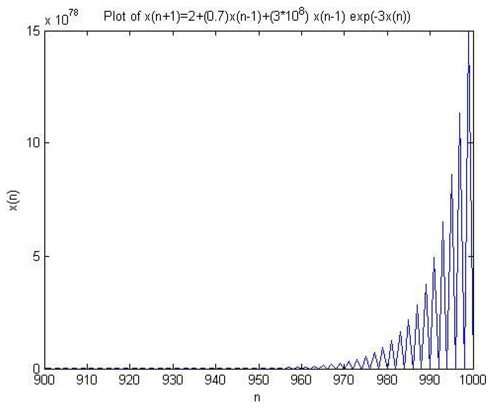
So, the equilibrium of (12) is global asymptotically stable. (See Figure 1 and Theorem 7).

Example 2.

We let ${\xi }_{-1}=0.1,{\xi }_0=1.3$, $a=2$, $b=0.7$, $c=3\times {10}^8$, and $\rho =3$. So, we deal with the equation

$${\xi }_{n+1}=2+0.7{\xi }_{n-1}+(3\times {10}^8){\xi }_{n-1}{e}^{-3{\xi }_n}.$$

(13)

Thus, the equilibrium of (13) is unstable. (See Figure 2).

7. Conclusions

We investigate the boundedness, local actions, and global asymptotic behavior of the solutions to the second-order difference equation of the exponential type

$${\xi }_{n+1}=a+b{\xi }_{n-1}+c{\xi }_{n-1}{e}^{-\rho {\xi }_n},$$

where $a,c,\rho \in (0,\infty )$, $b\in (0,1)$ and the initials ${\xi }_0,{\xi }_{-1}$ are non-negative real numbers. Our results generalized the results in [6]. We gave two concrete numerical examples to confirm the theoretical results.

References

- Ibrahim, T.F. Asymptotic behavior of a difference equation model in exponential form. Appear Math. Methods Appl. Sci. 2022. [Google Scholar] [CrossRef]
- Ibrahim, T.F.; Nurkanovic, Z. Kolmogorov-Arnold-Moser theory and symmetries for a polynomial quadratic second order difference equation. Mathematics 2019, 7, 790. [Google Scholar] [CrossRef]
- Ibrahim, T.F. Bifurcation and Periodically Semicycles for Fractional Difference Equation of fifth-order. J. Nonlinear Sci. Appl. 2018, 11, 375–382. [Google Scholar] [CrossRef]
- Ibrahim, T.F.; El-Moneam, M.A. Global stability of a higher-order difference equation. Iran. J. Sci. Technol. Trans. A Sci. 2017, 41, 51–58. [Google Scholar] [CrossRef]
- Ibrahim, T.F. Periodicity and Global Attractivity of Difference Equation of Higher-Order. J. Comput. Anal. Appl. 2014, 16, 552–564. [Google Scholar]
- El-Metwally, E.; Grove, E.A.; Ladas, G.; Levins, R.; Radin, M. On the difference equation ξn+1 = a + bξn−1e−ξn. Nonlinear Anal. 2001, 47, 4623–4634. [Google Scholar] [CrossRef]
- Ozturk, I.; Bozkurt, F.; Ozen, S. On the difference equation Appl. Math. Comput. 2006, 181, 1387–1393. [Google Scholar] [CrossRef]
- Ding, X.; Zhang, R. On the difference equation ξn+1 = (aξn + bξn−1)e−ξn. Adv. Differ. Equa. 2008, 2008, 876936. [Google Scholar]
- Gocen, M. On some difference equations of exponential form. Karaelmas Sci. Eng. J. 2018, 8, 581–584. [Google Scholar]
- Bo, Y.; Tian, D.; X, L.; Jin, Y.F. Discrete maximum principle and energy stability of the compact difference scheme for two-dimensional Allen-Cahn equation. J. Funct. Spaces 2022, 2022, 8522231. [Google Scholar] [CrossRef]
- Bozkurt, F. Stability analysis of a nonlinear difference equation. Int. Mod. Nonlinear Theory Appl. 2013, 2, 1–6. [Google Scholar] [CrossRef]
- Comert, T.; Yalcinkaya, I.; Tollu, D.T. A study on the positive solutions of an exponential type difference equation. Electron. Math. Anal. Appl. 2018, 6, 276–286. [Google Scholar]
- Feng, H.; Ma, H.; Ding, W. Global asymptotic behavior of positive solutions for exponential form difference equations with three parameters. Appl. Anal. Comput. 2016, 6, 600–606. [Google Scholar]
- Fotiades, N.; Papaschinopulos, G. Existence, uniqueness, and attractivity of prime period two solution for a difference equation of exponential form. Math. Comput. Model. 2012, 218, 11648–11653. [Google Scholar] [CrossRef]
- Khalsaraei, M.M.; Shokri, A.; Noeiaghdam, S.; Molayi, M. Nonstandard finite difference schemes for an SIR epidemic model. Mathematics 2021, 9, 23. [Google Scholar] [CrossRef]
- Ozturk, I.; Bozkurt, F.; Ozen, S. Global asymptotic behavior of the difference equation . Appl. Math. Lett. 2009, 22, 595–599. [Google Scholar] [CrossRef]
- Ragusa, M.A. Parabolic Herz spaces and their applications. Appl. Math. Lett. 2012, 25, 1270–1273. [Google Scholar] [CrossRef]
- Khan, A.Q.; Qureshi, M.N. Stability analysis of a discrete biological model. Int. J. Biomath. 2016, 9, 1650021. [Google Scholar] [CrossRef]
- Psarros, N.; Papaschinopoulos, G.; Papadopoulos, K.B. Long-term behavior of positive solutions of an exponentially self-regulating system of difference equations. Int. J. Biomath. 2017, 10, 1750045. [Google Scholar] [CrossRef]
- Kocic, V.L.; Ladas, G. Global Behavior of Nonlinear Difference Equations of Higher Order with Applications; Mathematics and Its Applications; Kluwer Academic Publishers: Dordrecht, The Netherlands, 1993; Volume 256. [Google Scholar]