

Molecular Collective Response and Dynamical Symmetry Properties in Biopotentials of Superior Plants: Experimental Observations and Quantum Field Theory Modeling

 ,
,  ,
,  and
and 
Abstract
:1. Introduction
2. Materials and Methods
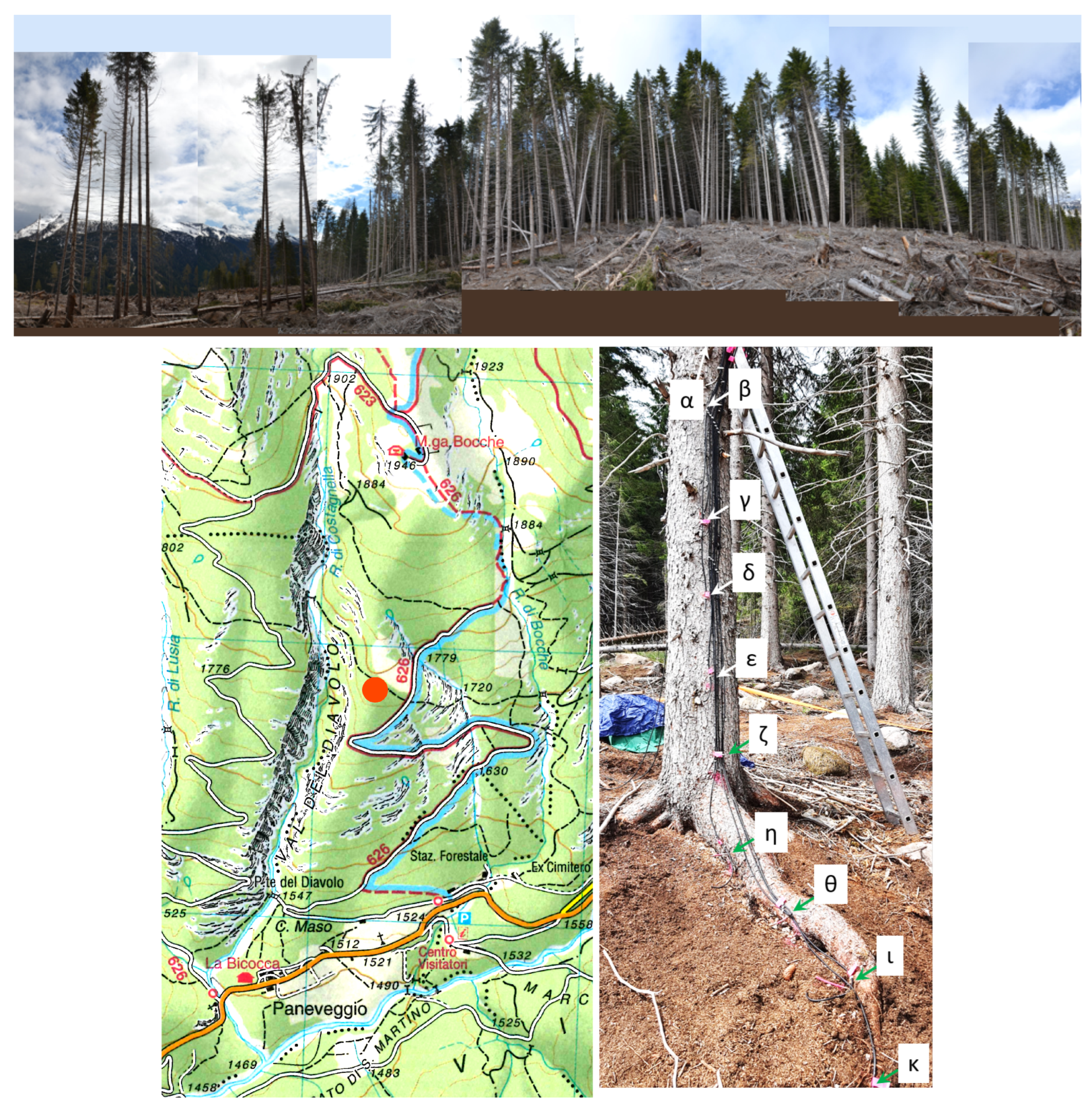
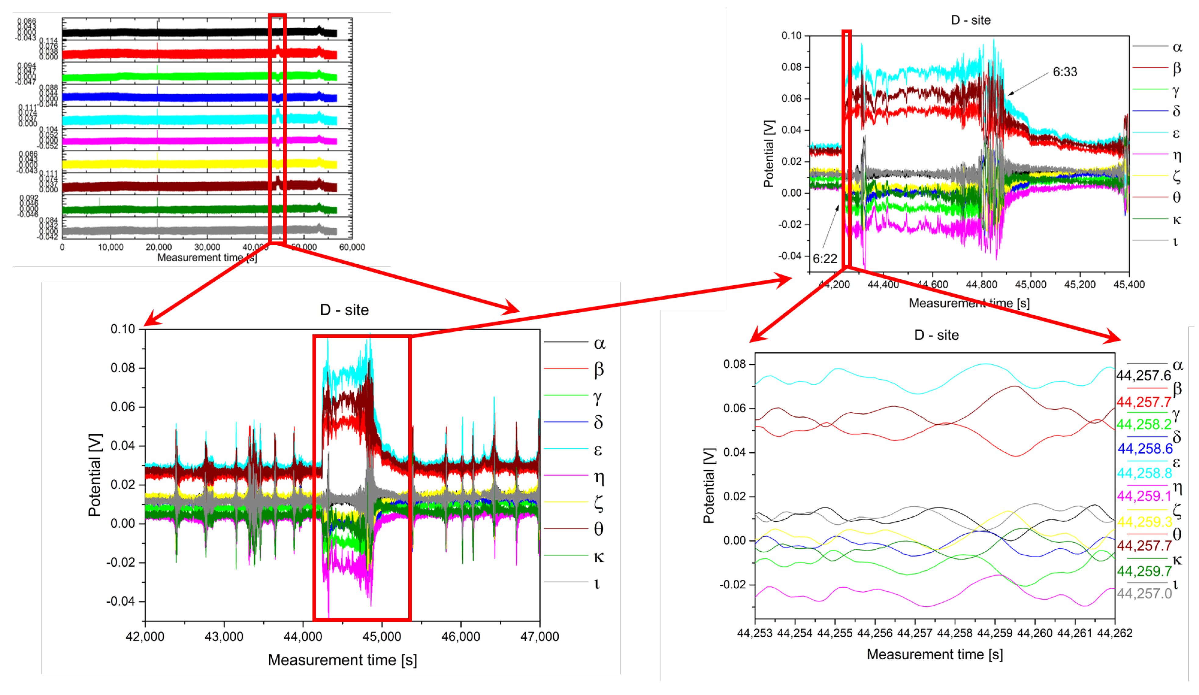
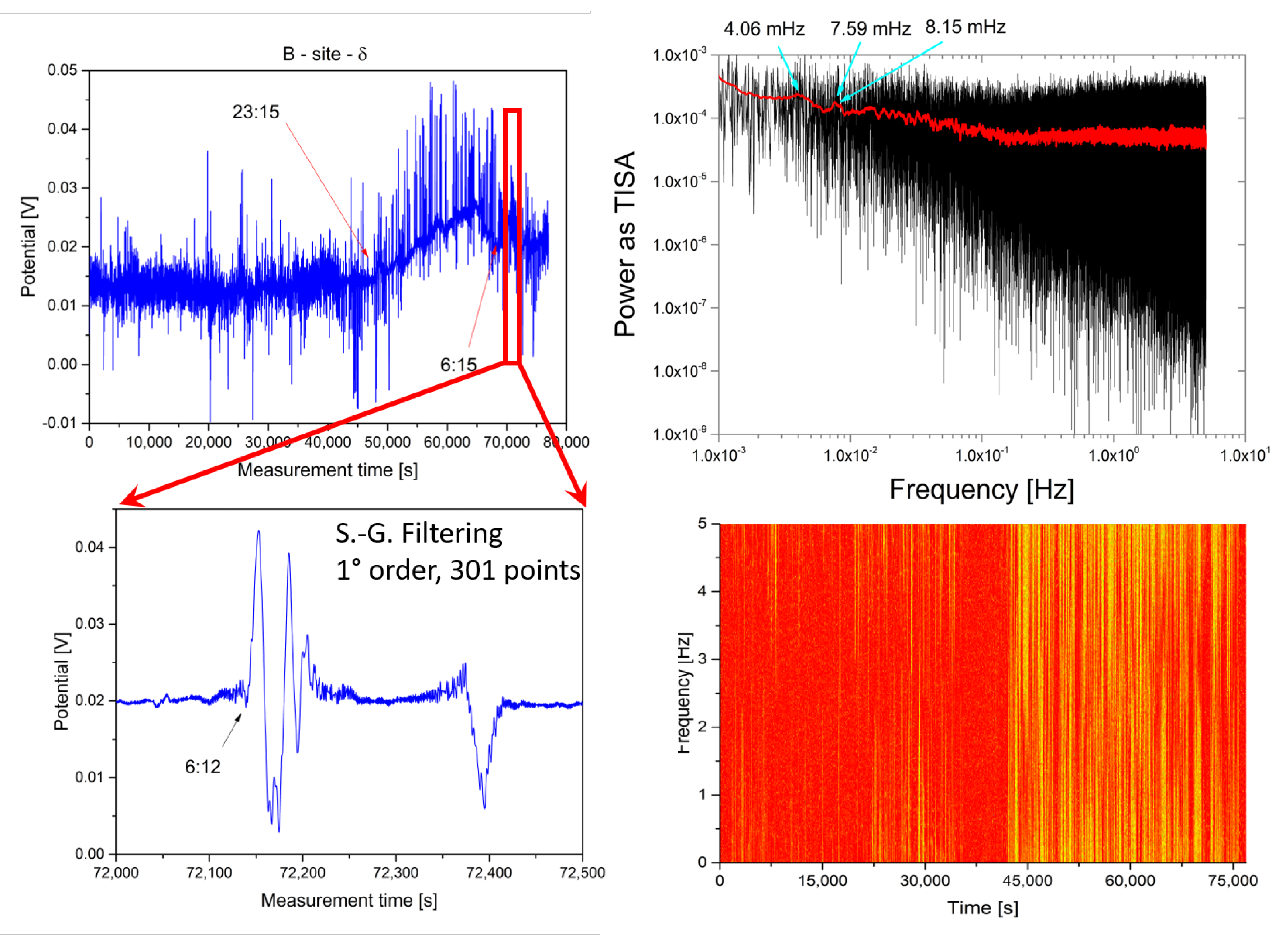
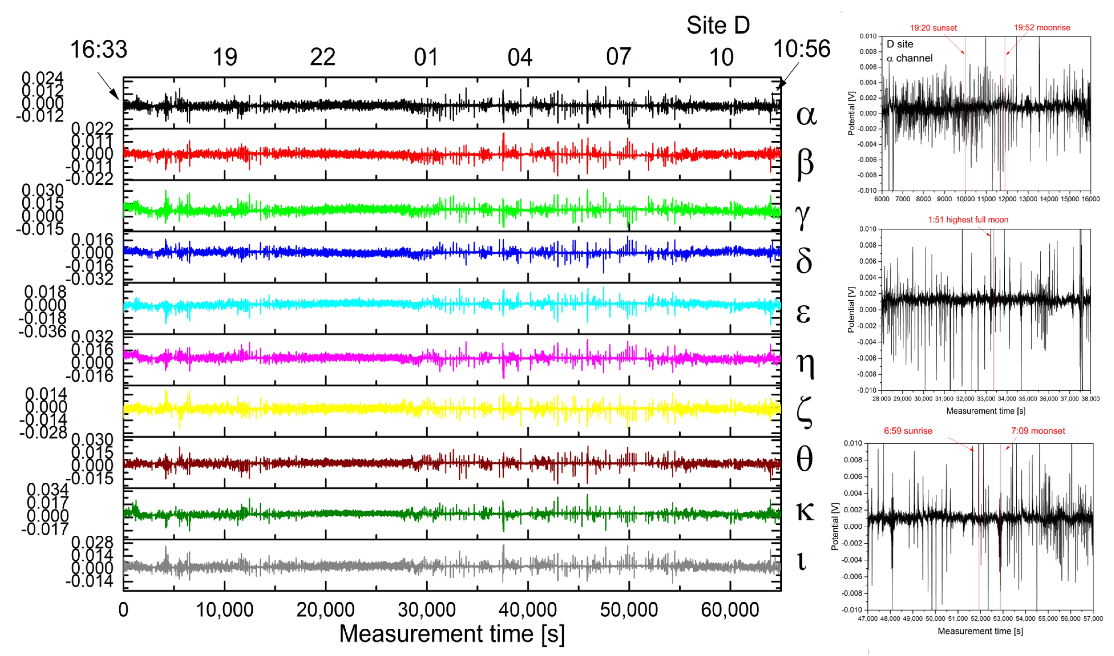
2.1. Experimental
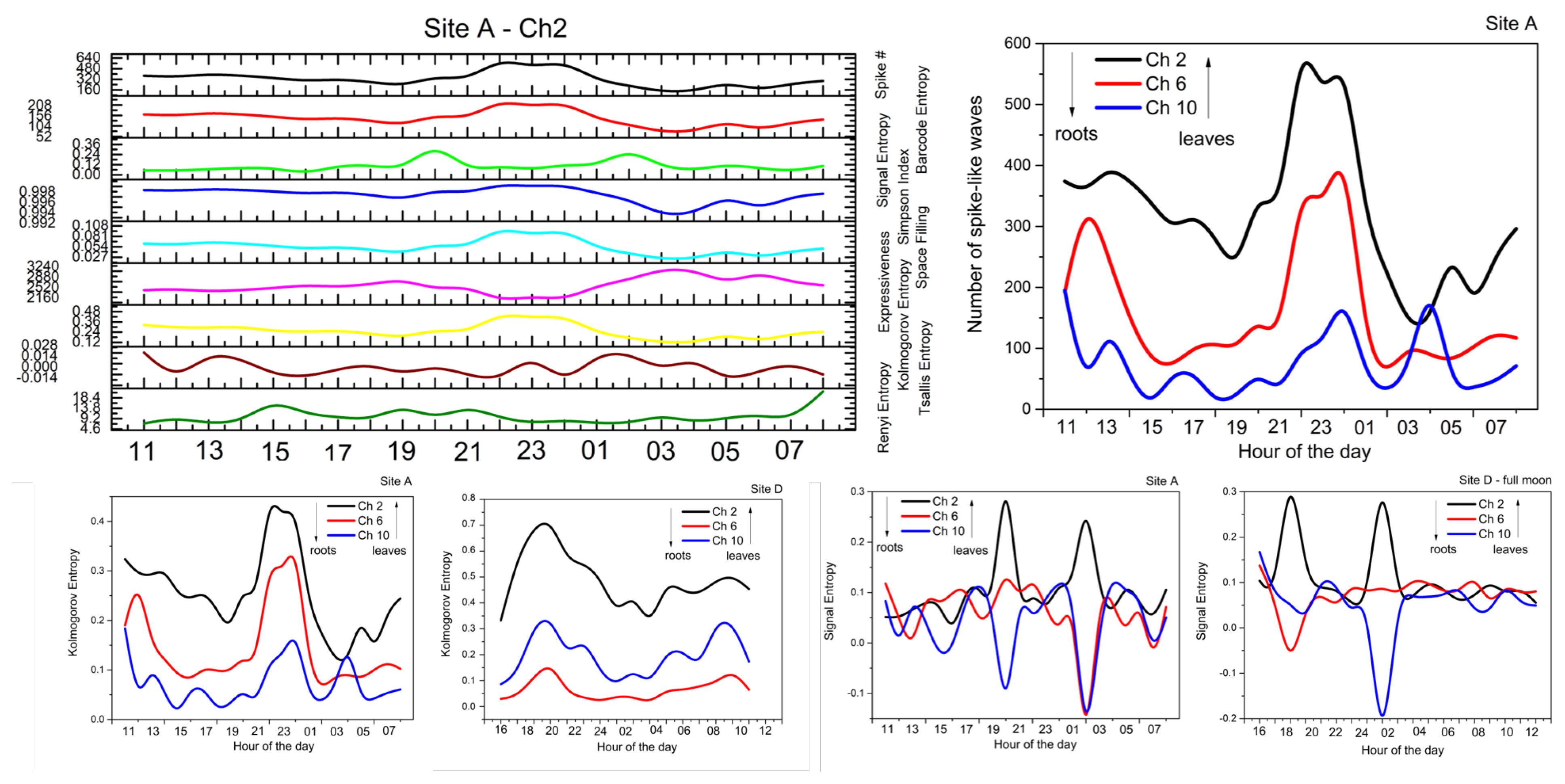
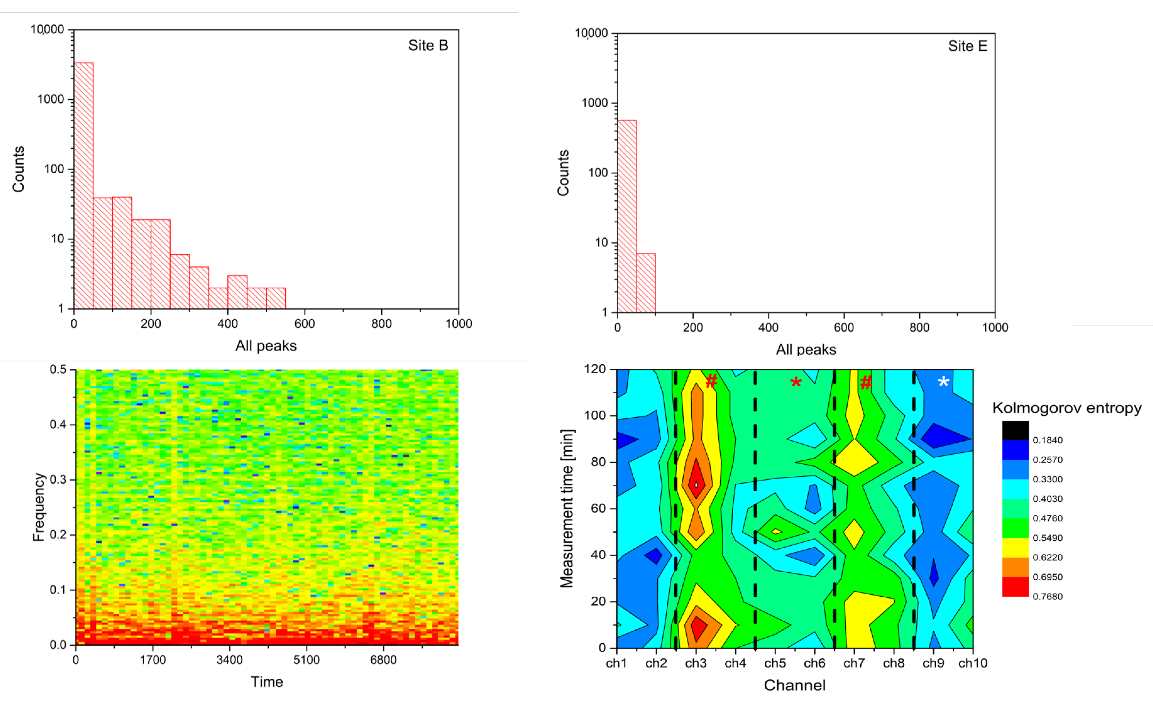
2.2. Analysis
- Spike number: Total number of located peaks.
- Barcode entropy: We represent the entire recording duration T with a binary string , with ‘1 s’ indicating the availability of spike events and ‘0 s’ otherwise. The Shannon entropy of this binary string (i.e., barcode entropy) is calculated by .
- Simpson index: It is calculated as . It linearly correlates with Shannon entropy for and the relationship becomes logarithmic for higher values of H. The value of ranges between 0 and 1, where 1 represents infinite diversity and 0 no diversity.
- Space filling (D) is the ratio of non-zero entries in W to the total length of string.
- Expressiveness (E) is calculated as the Shannon entropy H divided by space-filling ratio D, where it reflects the ‘economy of diversity’.
- Lempel–Ziv complexity () is used to assess temporal signal diversity, i.e., compressibility. We use the Kolmogorov complexity algorithm [24] to measure the Lempel–Ziv complexity.
- Rényi () [25] and Tsallis () [26] additive entropy concepts are generalizations of the classical Shannon entropy. Regardless of the generalization, these two entropy measurements are used in conjunction with the Principle of maximum entropy, with entropy’s main application being in statistical estimation theory. Tsallis and Rényi entropy measurements are expressed as and , where q is the entropic-index or Rényi entropy order with and , which in our experiments was set to 2.
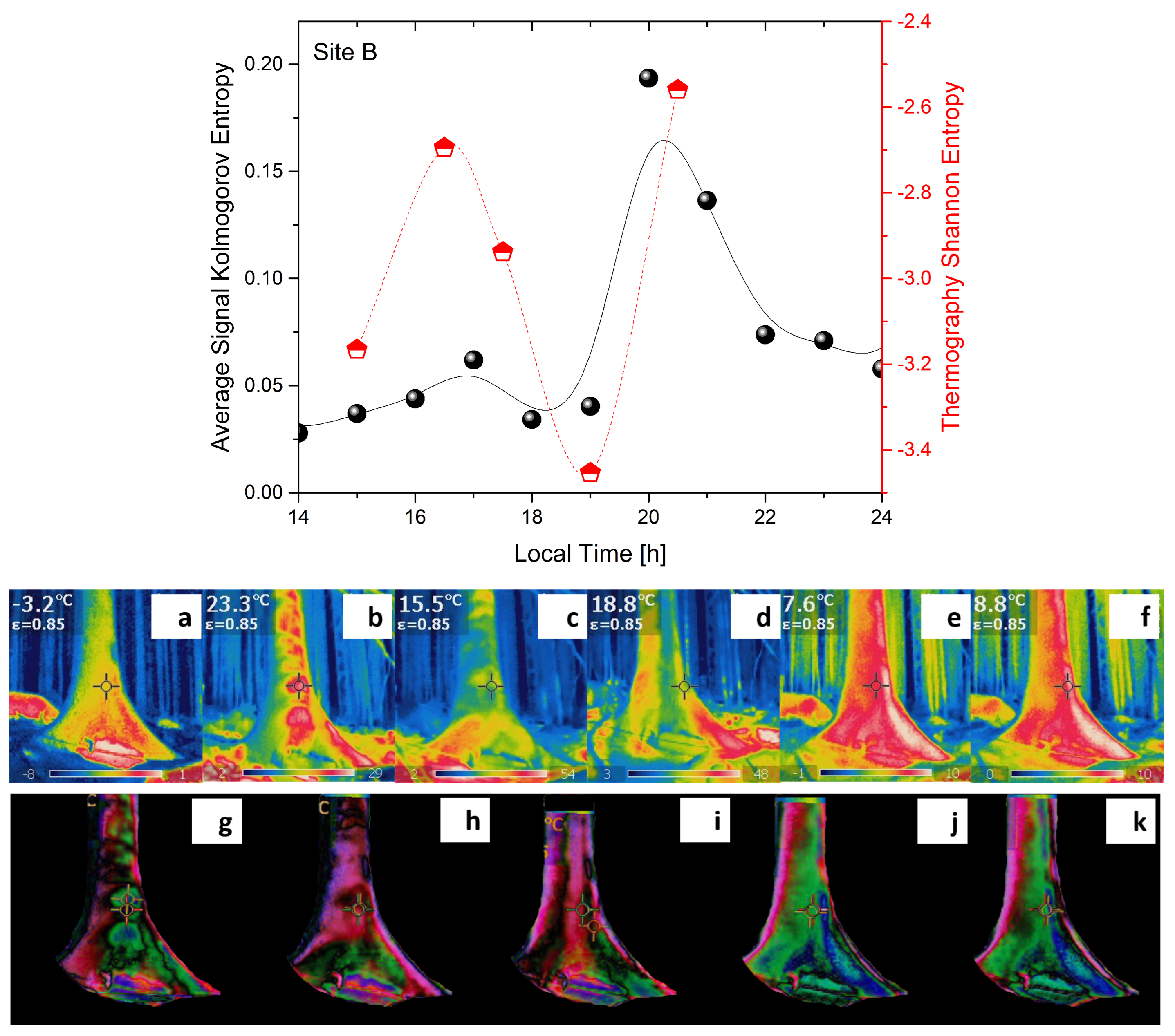
3. Results
3.1. Theoretical Modelling
3.1.1. Correlation Fields and Dissipative Dynamics
3.1.2. Electromagnetic Field and Collective Dynamical Effects
4. Conclusions and Future Prospects
Author Contributions
Funding
Institutional Review Board Statement
Informed Consent Statement
Data Availability Statement
Acknowledgments
Conflicts of Interest
Appendix A
Appendix A.1. Derivation of the Minimization of Free Energy from Equation (2)
Appendix A.2. Entropy, Free Energy and the Bose/Einstein Distribution Function
Appendix B
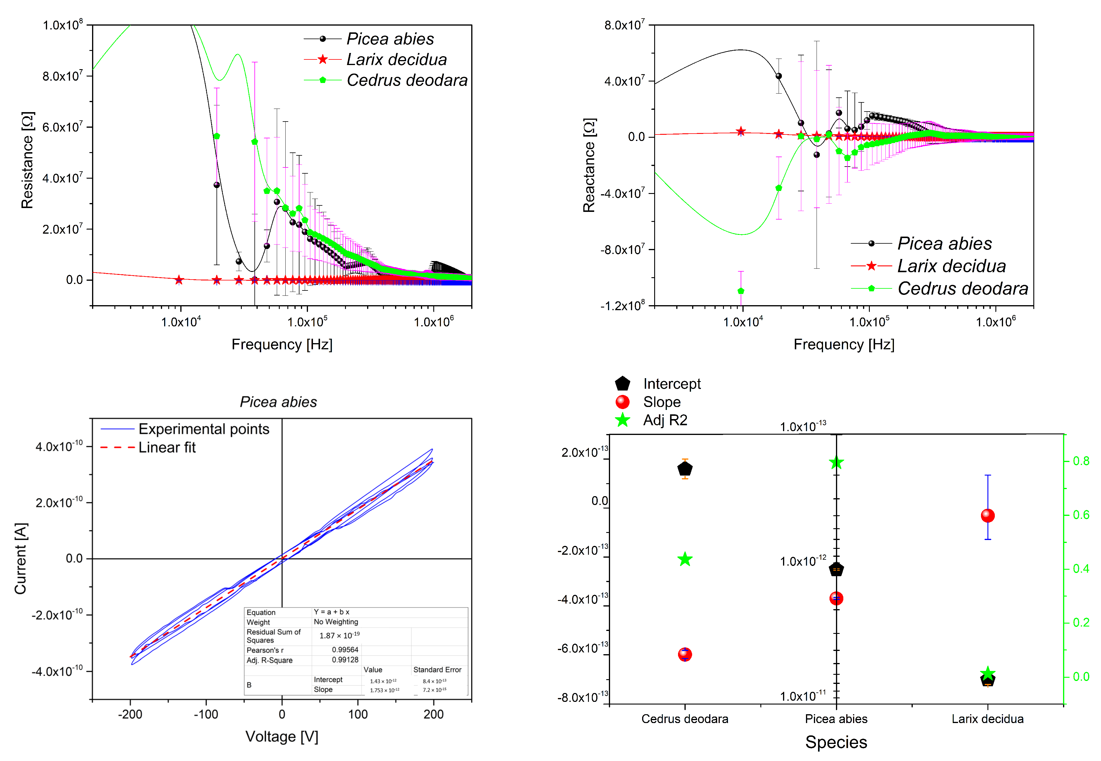
Appendix B.1. Resin Electrical Characterization
References
- Tallent-Halsell, N.G. Forest Health Monitoring: Field Methods Guide; Technical Report; Environmental Protection Agency: Las Vegas, NV, USA, 1994. [Google Scholar]
- Lausch, A.; Borg, E.; Bumberger, J.; Dietrich, P.; Heurich, M.; Huth, A.; Jung, A.; Klenke, R.; Knapp, S.; Mollenhauer, H.; et al. Understanding forest health with remote sensing, part III: Requirements for a scalable multi-source forest health monitoring network based on data science approaches. Remote Sens. 2018, 10, 1120. [Google Scholar] [CrossRef]
- Alexander, S.A.; Palmer, C.J. Forest health monitoring in the United States: First four years. Environ. Monit. Assess. 1999, 55, 267–277. [Google Scholar]
- Steinman, J. Tracking the health of trees over time on forest health monitoring plots. In Integrated Tools for Natural Resources Inventories in the 21st Century: An International Conference on the Inventory and Monitoring of Forested Ecosystems, 16–19 August 1998; Boise, ID. Gen. Tech. Rep. NCRS-212; Mark, H., Thomas, B., Eds.; US Department of Agriculture, Forest Service, North Central Research Station: St. Paul, MN, USA, 2000; pp. 334–339. [Google Scholar]
- Coulston, J.W.; Ambrose, M.J.; Riitters, K.H.; Conkling, B.L. Forest Health Monitoring: 2002 National Technical Report; Gen. Tech. Rep. SRS-84; US Department of Agriculture, Forest Service, Southern Research Station: Asheville, NC, USA, 2005; Volume 84, 97p. [Google Scholar]
- Carrière, S.; Ruffault, J.; Pimont, F.; Doussan, C.; Simioni, G.; Chalikakis, K.; Limousin, J.M.; Scotti, I.; Courdier, F.; Cakpo, C.B.; et al. Impact of local soil and subsoil conditions on inter-individual variations in tree responses to drought: Insights from Electrical Resistivity Tomography. Sci. Total Environ. 2020, 698, 134247. [Google Scholar] [CrossRef] [PubMed]
- Al Hagrey, S. Electrical resistivity imaging of tree trunks. Near Surf. Geophys. 2006, 4, 179–187. [Google Scholar] [CrossRef]
- Luo, Z.; Deng, Z.; Singha, K.; Zhang, X.; Liu, N.; Zhou, Y.; He, X.; Guan, H. Temporal and spatial variation in water content within living tree stems determined by electrical resistivity tomography. Agric. For. Meteorol. 2020, 291, 108058. [Google Scholar] [CrossRef]
- Ganthaler, A.; Sailer, J.; Bär, A.; Losso, A.; Mayr, S. Noninvasive Analysis of Tree Stems by Electrical Resistivity Tomography: Unraveling the Effects of Temperature, Water Status, and Electrode Installation. Front. Plant Sci. 2019, 10, 1455. [Google Scholar] [CrossRef] [PubMed]
- Brenner, E.D.; Stahlberg, R.; Mancuso, S.; Vivanco, J.; Baluška, F.; Van Volkenburgh, E. Plant neurobiology: An integrated view of plant signaling. Trends Plant Sci. 2006, 11, 413–419. [Google Scholar] [CrossRef]
- Baluška, F.; Mancuso, S.; Volkmann, D. Communication in Plants: Neuronal Aspects of Plant Life; Springer: Berlin/Heidelberg, Germany, 2006. [Google Scholar]
- Mancuso, S.; Viola, A. Brilliant Green: The Surprising History and Science of Plant Intelligence; Island Press: Washington, DC, USA, 2015. [Google Scholar]
- Grant, R. Do trees talk to each other? Smithson. Mag. 2018, 180968084, 1–9. [Google Scholar]
- Baluška, F.; Mancuso, S. Plant neurobiology: From sensory biology, via plant communication, to social plant behavior. Cogn. Process. 2009, 10, 3–7. [Google Scholar] [CrossRef]
- Hedrich, R.; Salvador-Recatalà, V.; Dreyer, I. Electrical wiring and long-distance plant communication. Trends Plant Sci. 2016, 21, 376–387. [Google Scholar] [CrossRef]
- Gorzelak, M.A.; Asay, A.K.; Pickles, B.J.; Simard, S.W. Inter-plant communication through mycorrhizal networks mediates complex adaptive behaviour in plant communities. AoB Plants 2015, 7, plv050. [Google Scholar] [CrossRef]
- Hanson, A. Spontaneous electrical low-frequency oscillations: A possible role in Hydra and all living systems. Philos. Trans. R. Soc. B Biol. Sci. 2021, 376, 20190763. [Google Scholar] [CrossRef]
- Volkov, A.G.; Shtessel, Y.B. Underground electrotonic signal transmission between plants. Commun. Integr. Biol. 2020, 13, 54–58. [Google Scholar] [CrossRef]
- Adamatzky, A. Language of fungi derived from their electrical spiking activity. R. Soc. Open Sci. 2022, 9, 211926. [Google Scholar] [CrossRef]
- Tattoni, C.; Ciolli, M.; Ferretti, F.; Cantiani, M.G. Monitoring spatial and temporal pattern of Paneveggio forest (northern Italy) from 1859 to 2006. iForest-Biogeosci. For. 2010, 3, 72. [Google Scholar] [CrossRef]
- Auricchio, L.; Cook, E.; Pacini, G. ‘Fatto di Fiemme’: Stradivari’s violins and the musical trees of the Paneveggio. In Invaluable Trees: Cultures of Nature; Voltaire Foundation: Oxford, UK, 2012. [Google Scholar]
- Burckle, L.; Grissino-Mayer, H.D. Stradivari, violins, tree rings, and the Maunder Minimum: A hypothesis. Dendrochronologia 2003, 21, 41–45. [Google Scholar] [CrossRef]
- Cherubini, P. Tree-ring dating of musical instruments. Science 2021, 373, 1434–1436. [Google Scholar] [CrossRef]
- Kaspar, F.; Schuster, H. Easily calculable measure for the complexity of spatiotemporal patterns. Phys. Rev. A 1987, 36, 842. [Google Scholar] [CrossRef]
- Rényi, A. On measures of entropy and information. In Proceedings of the Fourth Berkeley Symposium on Mathematical Statistics and Probability, Volume 1: Contributions to the Theory of Statistics; University of California Press: Berkeley, CA, USA, 1961; pp. 547–561. [Google Scholar]
- Tsallis, C. Possible generalization of Boltzmann-Gibbs statistics. J. Stat. Phys. 1988, 52, 479–487. [Google Scholar] [CrossRef]
- Matsumoto, H.; Umezawa, H.; Vitiello, G.; Wyly, J. Spontaneous breakdown of a non-Abelian symmetry. Phys. Rev. 1974, D9, 2806–2813. [Google Scholar] [CrossRef]
- Shah, M.; Umezawa, H.; Vitiello, G. Relation among spin operators and magnons. Phys. Rev. 1974, B10, 4724–4726. [Google Scholar] [CrossRef]
- Matsumoto, H.; Papastamatiou, N.J.; Umezawa, H.; Vitiello, G. Dynamical rearrangement in Anderson-Higgs-Kibble mechanism. Nucl. Phys. B 1975, 97, 61–89. [Google Scholar] [CrossRef]
- Del Giudice, E.; Doglia, S.; Milani, M.; Vitiello, G. A quantum field theoretical approach to the collective behaviour of biological systems. Nucl. Phys. B 1985, 251, 375–400. [Google Scholar] [CrossRef]
- Del Giudice, E.; Doglia, S.; Milani, M.; Vitiello, G. Electromagnetic field and spontaneous symmetry breaking in biological matter. Nucl. Phys. B 1986, 275, 185–199. [Google Scholar] [CrossRef]
- Itzykson, C.; Zuber, J. Electromagnetic Field and Spontaneous Symmetry Breaking in Biological Matter; McGraw-Hill: New York, NY, USA, 1980. [Google Scholar]
- Umezawa, H.; Matsumoto, H.; Tachiki, M. Thermo Field Dynamics and Condensed States; North-Holland: Amsterdam, The Netherlands, 1982. [Google Scholar]
- Umezawa, H. Advanced Field Theory: Micro, Macro, and Thermal Physics; AIP: New York, NY, USA, 1993. [Google Scholar]
- Blasone, M.; Jizba, P.; Vitiello, G. Quantum Field Theory and Its Macroscopic Manifestations; Imperial College Press: London, UK, 2011. [Google Scholar]
- Fermi, E. Termodinamica; Boringhieri: Torino, Italy, 1958. [Google Scholar]
- Landau, L.; Lifshitz, E.M. Statistical Physics; Pergamon Press: Oxford, UK, 1958. [Google Scholar]
- Kurcz, A.; Capolupo, A.; Beige, A.; Del Giudice, E.; Vitiello, G. Energy concentration in composite quantum systems. Phys. Rev. A 2010, 81, 063821. [Google Scholar] [CrossRef]
- Matsumoto, H.; Papastamatiou, N.J.; Umezawa, H. The boson transformation and the vortex solutions. Nucl. Phys. B 1975, 97, 90–124. [Google Scholar] [CrossRef]
- Lechelon, M.; Meriguet, Y.; Gori, M.; Ruffenach, S.; Nardecchia, I.; Floriani, E.; Coquillat, D.; Teppe, F.; Mailfert, S.; Marguet, D.; et al. Experimental evidence for long-distance electrodynamic intermolecular forces. Sci. Adv. 2022, 8, eabl5855. [Google Scholar] [CrossRef]
- Celeghini, E.; Rasetti, M.; Vitiello, G. Quantum Dissipation. Ann. Phys. 1992, 215, 156–170. [Google Scholar] [CrossRef]
- Perelomov, A. Generalized Coherent States and Their Applications; Springer: Berlin/Heidelberg, Germany, 1986. [Google Scholar]
- Hilborn, R. Chaos and Nonlinear Dynamics; Oxford University Press: Oxford, UK, 1994. [Google Scholar]
- Gerry, C.; Knight, P. Introductory Quantum Optics; Cambridge University Press: Cambridge, UK, 2005. [Google Scholar]
- Sabbadini, S.; Vitiello, G. Entanglement and phase-mediated correlations in quantum field theory. Application to brain-mind states. Appl. Sci. 2019, 9, 3203. [Google Scholar] [CrossRef]
- Lee, R.A. The Stability of Wood Resin Colloids in Paper Manufacture. Ph.D. Thesis, University of Tasmania, Hobart, Australia, 2012. [Google Scholar]
- Douros, A.; Christopoulou, A.; Kikionis, S.; Nikolaou, K.; Skaltsa, H. Volatile Components of Heartwood, Sapwood, and Resin from a Dated Cedrus brevifolia. Nat. Prod. Commun. 2019, 14. [Google Scholar] [CrossRef] [Green Version]

Publisher’s Note: MDPI stays neutral with regard to jurisdictional claims in published maps and institutional affiliations. |
© 2022 by the authors. Licensee MDPI, Basel, Switzerland. This article is an open access article distributed under the terms and conditions of the Creative Commons Attribution (CC BY) license (https://creativecommons.org/licenses/by/4.0/).
Share and Cite
Chiolerio, A.; Dehshibi, M.M.; Vitiello, G.; Adamatzky, A. Molecular Collective Response and Dynamical Symmetry Properties in Biopotentials of Superior Plants: Experimental Observations and Quantum Field Theory Modeling. Symmetry 2022, 14, 1792. https://doi.org/10.3390/sym14091792
Chiolerio A, Dehshibi MM, Vitiello G, Adamatzky A. Molecular Collective Response and Dynamical Symmetry Properties in Biopotentials of Superior Plants: Experimental Observations and Quantum Field Theory Modeling. Symmetry. 2022; 14(9):1792. https://doi.org/10.3390/sym14091792
Chicago/Turabian StyleChiolerio, Alessandro, Mohammad Mahdi Dehshibi, Giuseppe Vitiello, and Andrew Adamatzky. 2022. "Molecular Collective Response and Dynamical Symmetry Properties in Biopotentials of Superior Plants: Experimental Observations and Quantum Field Theory Modeling" Symmetry 14, no. 9: 1792. https://doi.org/10.3390/sym14091792
APA StyleChiolerio, A., Dehshibi, M. M., Vitiello, G., & Adamatzky, A. (2022). Molecular Collective Response and Dynamical Symmetry Properties in Biopotentials of Superior Plants: Experimental Observations and Quantum Field Theory Modeling. Symmetry, 14(9), 1792. https://doi.org/10.3390/sym14091792