Bivariate Step-Stress Accelerated Life Tests for the Kavya–Manoharan Exponentiated Weibull Model under Progressive Censoring with Applications

Abstract

A new three-parameter survival model is proposed using the Kavya–Manoharan (KM) transformation family and the exponentiated Weibull (EW) distribution. The shapes of the pdf for the new model can be asymmetric and symmetric shapes, such as unimodal, decreasing, right-skewed and symmetric. In addition, the shapes of the hrf for the suggested model can be increasing, decreasing, constant and J-shaped. Statistical properties are obtained: quantile function, mode, moments, incomplete moments, residual life time, reversed residual life time, probability weighted moments, order statistics and entropy. We discuss the maximum likelihood estimation for the model. The relevance and flexibility of the model are demonstrated using two real datasets. The distribution is very flexible, and it outperforms many known distributions, such as the three-parameter exponentiated Weibull, the modified Weibull model, the Kavya–Manoharan Weibull, the extended Weibull, the odd Weibull inverse Topp–Leone and the extended odd Weibull inverse Nadarajah–Haghigh model. A bivariate step-stress accelerated life test based on progressive type-I censoring (PTIC) using the model is presented. This pattern is noticed when a particular number of lifetime test units are routinely eliminated from the test at the conclusion of each post-test period of time. Minimizing the asymptotic variance of the MLE of the log of the scale parameter at design stress under PTIC yields an expression for the ideal test plan under PTIC.

1. Introduction

In order to enhance survival data modeling, statisticians and applied researchers have been increasingly interested in developing flexible lifetime models. As a consequence, significant progress has been achieved in generalizing and applying a number of well-known lifetime models. The Weibull distribution, introduced by Weibull [1], is one of the most used distributions for modeling lifetimes. The Weibull has been utilized effectively as a purely empirical model in many applications due to its flexible form and ability to predict a wide variety of failure rates. The Weibull model may be theoretically developed as a type of extreme value distribution that governs the time until occurrence of the “weakest link” among several competing failure processes. This might account for its performance in applications such as capacitor, ball bearing, relay and material strength failures. The hazard rate function (hrf) of the Weibull distribution can only be increasing, decreasing or constant. As a result, it is not useful for modeling human mortality or machine lifetimes with a non-monotonic hrf. Many variants that generalize the Weibull distribution have emerged. Mudholkar et al. [2] were the first to extend the Weibull distribution with a bathtub-shaped hazard rate, and this extended Weibull has been successfully applied by Xie et al. [3]. Other extensions and modified forms of the Weibull with greater flexibility have been proposed; for example, the additive Weibull distribution with a bathtub-shaped hrf by Xie and Lai [4], the EW distribution by Nadarajah et al. [5], the transmuted additive Weibull by Elbatal et al. [6], the Kumaraswamy transmuted exponentiated modified Weibull by Al-Babtain et al. [7], the Burr X EW model by Khalil et al. [8], the Marshall–Olkin power-generalized Weibull distribution by Afify et al. [9], truncated Cauchy power Weibull-G by Alotaibi et al. [10], a new version of Weighted Weibull distribution by Alahmadi et al. [11], exponentiated power generalized Weibull power series family by Aldahlan et al. [12], exponentiated truncated inverse Weibull-G by Almarashi et al. [13], odd inverse power generalized Weibull by Al-Moisheer et al. [14], extended inverse Weibull distribution by Alkarni et al. [15], four-parameter Weibull distribution by Abouelmagd et al. [16], exponentiated Weibull Weibull distribution by Hassan and Elgarhy [17] among others.

Mudholkar and Srivastava [18] presented the three-parameter EW distribution as an extension of the Weibull family, which is a particularly flexible class of probability distribution functions. Mudholkar et al. [2] demonstrated the use of the EW distribution in reliability and survival tests.

The cumulative function (cdf) and density function (pdf) of the EW model are given by

$$G_{{}_{EW}}(x;\alpha ,\beta ,\theta )={\left[1-e^{-{\left(\alpha x\right)}^{\beta }}\right]}^{\theta },x>0,\alpha ,\beta ,\theta >0$$

(1)

and

$$g_{{}_{EW}}(x;\alpha ,\beta ,\theta )=\beta \theta {\alpha }^{\beta }{x}^{\beta -1}{e}^{-{\left(\alpha x\right)}^{\beta }}{\left[1-e^{-{\left(\alpha x\right)}^{\beta }}\right]}^{\theta -1},$$

(2)

where $\beta$ and $\theta$ are two shape parameters and $\alpha$ is the scale parameter. For $\beta =1$, it represents the exponentiated exponential (EE) distribution, for $\beta =2$, it represents the exponentiated Rayleigh (ER) distribution, for $\beta =\theta =1$, it represents the exponential (E) distribution, for $\beta =2,\theta =1$, it represents the Rayleigh (R) distribution [19] and for $\theta =1$, it represents the Weibull distribution. Thus, EW is a generalization of the EE distribution, as well as the Weibull distribution. The EW distribution also has a very good physical interpretation.

We have three reasons for using the EW distribution. First, it expands the popular Weibull and EE models. Second, the hazard rate function of this distribution has several forms, one of which is the bathtub form. As a result, it could be a helpful distribution for analyzing biological and mortality data. Third, if a parallel system has n components and their lifetimes are independently and identically distributed as EW, then the system lifetime is also EW.

Additional parameters give greater flexibility, but they also increase the complexity of the estimation. To counter this, ref. [20] proposed the Dinesh–Umesh–Sanjay (DUS) transformation to obtain new parsimonious classes of distributions. This is as follows. If $G\left(x\right)$ is the baseline cdf, the DUS transformation generates a new cdf $F\left(x\right)$ expressed as

$$F\left(x\right)=\frac{e^{G\left(x\right)}-1}{e-1}.$$

The merit of using this transformation is that the resulting distribution is parameter-parsimonious because no extra parameters are added. In this way, Maurya et al. [21] proposed a new class of distributions that includes many flexible hazard rates. They explored using the DUS transformation by using the exponentiated cdf, introducing the generalized DUS (GDUS) transformation. Kavya and Manoharan [22] proposed a generalized lifetime model based on the DUS transformation, with the cdf of the GDUS transformation given by

$$F(x;\alpha ,\zeta )=\frac{exp\left(G^{\alpha }(x;\zeta )\right)-1}{e-1},x>0,$$

where $\alpha >0.$ The associated pdf is given by

$$f(x;\alpha ,\zeta )=\frac{\alpha g\left(x;\zeta \right)G^{\alpha -1}(x;\zeta )exp\left(G^{\alpha }(x;\zeta )\right)}{e-1},$$

where $G(x;\zeta )$ is the baseline distribution in the $GDUS$ family distribution. This approach will always create a parsimonious distribution because it is a transformation rather than a generalization, so no additional parameters beyond those in the baseline distribution are introduced.

Recently, Kavya and Manoharan [23] introduced a new transformation, the KM transformation family of distributions. The cdf and pdf are, respectively,

$$F_{{}_{KM}}\left(x\right)=\frac{e}{e-1}\left(1-e^{-G\left(x\right)}\right),x>0,$$

(3)

and

$$f_{KM}\left(x\right)=\frac{e}{e-1}g\left(x\right)e^{-G\left(x\right)}.$$

(4)

The hrf is provided via

$${\xi }_{{}_{KM}}\left(x\right)=\frac{g\left(x\right)e^{1-G\left(x\right)}}{e^{1-G\left(x\right)}-1}.$$

(5)

Using a given baseline distribution, this family generates new lifetime models or distributions.

Kavya and Manoharan [23] used the exponential and Weibull distributions as baseline distributions because they are widely used in reliability theory and survival analysis.

Censored data arise in real-world testing trials when investigations, including the lifetime of test units, must be terminated before complete observation. Censoring is a common and unavoidable routine activity for a variety of reasons, including time restrictions and cost savings. Censorship in its different forms has been carefully examined, with types I and II censorship being the most prevalent. In comparison to traditional censorship designs, a generalized censorship style known as progressive censored schemes has recently attracted substantial attention in the literature due to its efficient use of available resources. One of these progressive censored schemes is the PTIC. This pattern is noticed when a particular number of lifetime test units are routinely eliminated from the test at the conclusion of each post-test period of time. It has the capacity to determine the termination time realistically and there is additional design freedom by allowing test units to be terminated during non-terminal time periods, as studied by Balakrishnan et al. [24]. Bayesian and classical inference for an odd Lindley Burr XII model are proposed in the study by Korkmaz et al. [25] and Topp–Leone NH distribution is proposed in the study by Yousof et al. [26].

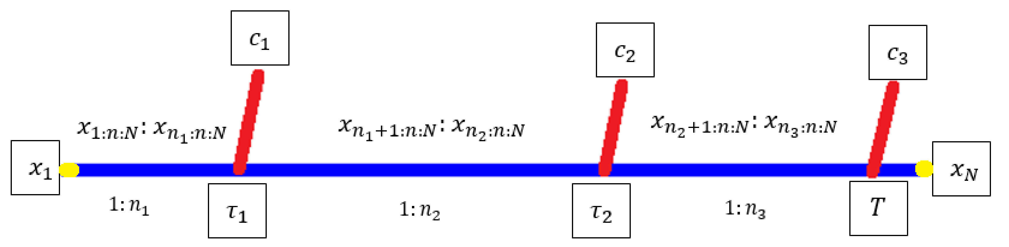
Suppose that a life testing experiment has n units. Presume that $X_1,X_2,\dots ,X_n$ represent the lifetime of all n units taken from a population. Assume that $x_{\left(1\right)}<x_{\left(2\right)}<\dots <x_{\left(n\right)}$ denotes the respective ordered lifetime recorded from the life test. At the end of the preset period of censoring $Tqi$, $Ri$ items are excluded from the surviving items in accordance with $q{i}^{th}$ Qs, $i=1,2,\dots ,m$, where m signifies the number of testing phases, $T_{q_i}>T_{q_{i-1}}$ and $n=r+{\sum }_{i=1}^m{R}_i$.

The quantities $T_{q_i}$ should always be determined ahead of time:

• Predicated on the experimenter’s past knowledge and skills with the objects under consideration, as in the study by Balasooriya and lwa [27];
• Or the quantiles of the lifetimes distribution, $qi$th, which are possibly computed by using the provided expression

  $$P(X\le T_{q_i})=q_i\Rightarrow T_{q_i}=F^{-1}\left(q_i\right)i=1,2,\dots ,m.$$

Within those cases, $Ri,Tqi$ and n are fixed and constant, whereas $li$ represents the quantity of surviving entities at a particular moment in time, and $Tqi$ and $r=\sum {i=1}^{m}li$ are random variables. The likelihood function is represented as

$$\ell (\theta )\propto \prod _{i=1}^{r}f\left(x_{\left(i\right)}\right)\prod _{k=1}^s{\left(1-F\left(T_{\left(q_k\right)}\right)\right)}^{R_k}$$

wherein $x\left(i\right)$ is the observable lifetime of the ith OS [28]. This censorship mechanism is depicted in Figure 1; see Balakrishnan and Cramer [29]. The type-I and type-II conventional censoring methods are generalized by these progressive censoring schemes, which also allow for partial withdrawals from the ongoing experiment. The fact that they assume a constant review of the life test experiment is a significant problem with these progressive censoring schemes, as well as with all other classic censoring schemes.

Complete samples, as well as the type-I censoring scheme, can indeed be viewed as special examples of this censoring technique.

The PTIC approach for the Weibull distribution was proposed in the study by Balakrishnan and Cramer [29]. The maximum likelihood estimates (MLEs) and Bayesian estimates for the unknown parameters of the generalized inverse exponential distribution under PTIC were obtained in the study by Mahmoud et al. [30]. Abo-Kasem et al. [31] discussed inferential survival analysis for inverted NH distribution under adaptive progressive hybrid censoring. For the PTIC, there are two publications that are closely linked. The first was the MLEs and asymptotic confidence estimates for the parameters of the extended inverse exponential model, predicated on the premise that there are two kinds of failures, as in the study by Mahmoud et al. [32]. Ahmad et al. [33] discussed inference on reliability estimation for a multi-component stress-strength model under power Lomax distribution. Almetwally et al. [34] obtained the best optimal plan of multi-stress–strength reliability Bayesian and non-Bayesian methods for the alpha power exponential model using progressive first failure. The second was the MLEs and Bayesian estimates for the unknown parameters of the extended inverse exponential model, as in the study by Mahmoud et al. [35]. Algarni et al. [36] investigate the statistical inference of the inverse Weibull model under PTIC. Elbatal et al. [37] investigate the Bayesian and non-Bayesian estimation of the Nadarajah–Haghighi distribution under PTIC.

Turning now to accelerated life tests (ALTs), these are a means of gathering more information in less time than would otherwise be possible by subjecting items to more stress than in usual operating conditions. Such testing can save a significant amount of time and money. The step-stress accelerated life test (SSALT) is one type of ALT; see Hakamipour [38]. During the test, the experimenter progressively increases the stress levels at pre-specified time intervals, typically starting with a stress level that is slightly above normal condition. The test continues until either the entire sample of items fails or the time limit for the duration of the test is reached and censoring occurs.

When stress(es) are applied items in only two phases, this is referred to as a simple SSALT. Meeker [39], as well as Nelson [40], are good resources for interested readers. Many different types of SSALT censorship have been used in the literature. El-Sherpieny et al. [41] introduced PTIIC for bivariate distributions based on ALT. The bulk of these studies concentrate on types I and II censoring. When items are eliminated before they fail on test, the cost of the test is lowered since these deleted samples can be utilized elsewhere or in other tests. This is referred to as progressive censorship. Most tests employ just one accelerating stress variable. It is recommended to employ many stress factors since using only one variable may result in insufficient failure data. Increasing the number of stress components would result in a better knowledge of the simultaneous effects of the stress variables, as well as more failure data.

Han [42] addressed the best design of a basic SSALT for an exponential distribution using PTIC. Li and Fard [43] investigated SSALT for two stress variables using Weibull failure times and type-I censoring. To obtain optimal hold durations, Ling et al. [44] built an SSALT for two stress variables in a type-I hybrid censoring scheme. “Bivariate SSALT” refers to an SSALT with two stress components; for more details of this scheme, see Figure 2. The study by [45] obtained the best design for a bivariate SSALT model with type-II censoring for the Gompertz distribution. Hakamipour [38] discussed the optimum design for a bivariate SSALT with a generalized exponential distribution under PTIC. Khan and Chandra [46] discussed bivariate SSALT estimation and the optimum design under PTIC. Alotaibi et al. [47] introduced the optimal design for a bivariate SSALT for alpha power exponential distribution based on PTIC samples. The test is repeated until T is attained, at which time, $n_2$ units fail this stage. At time T, all of the remaining surviving units $c_3=N-n_1-c_1-n_2-c_2-n_3$ are removed from the test. For more explanation, see Figure 2.

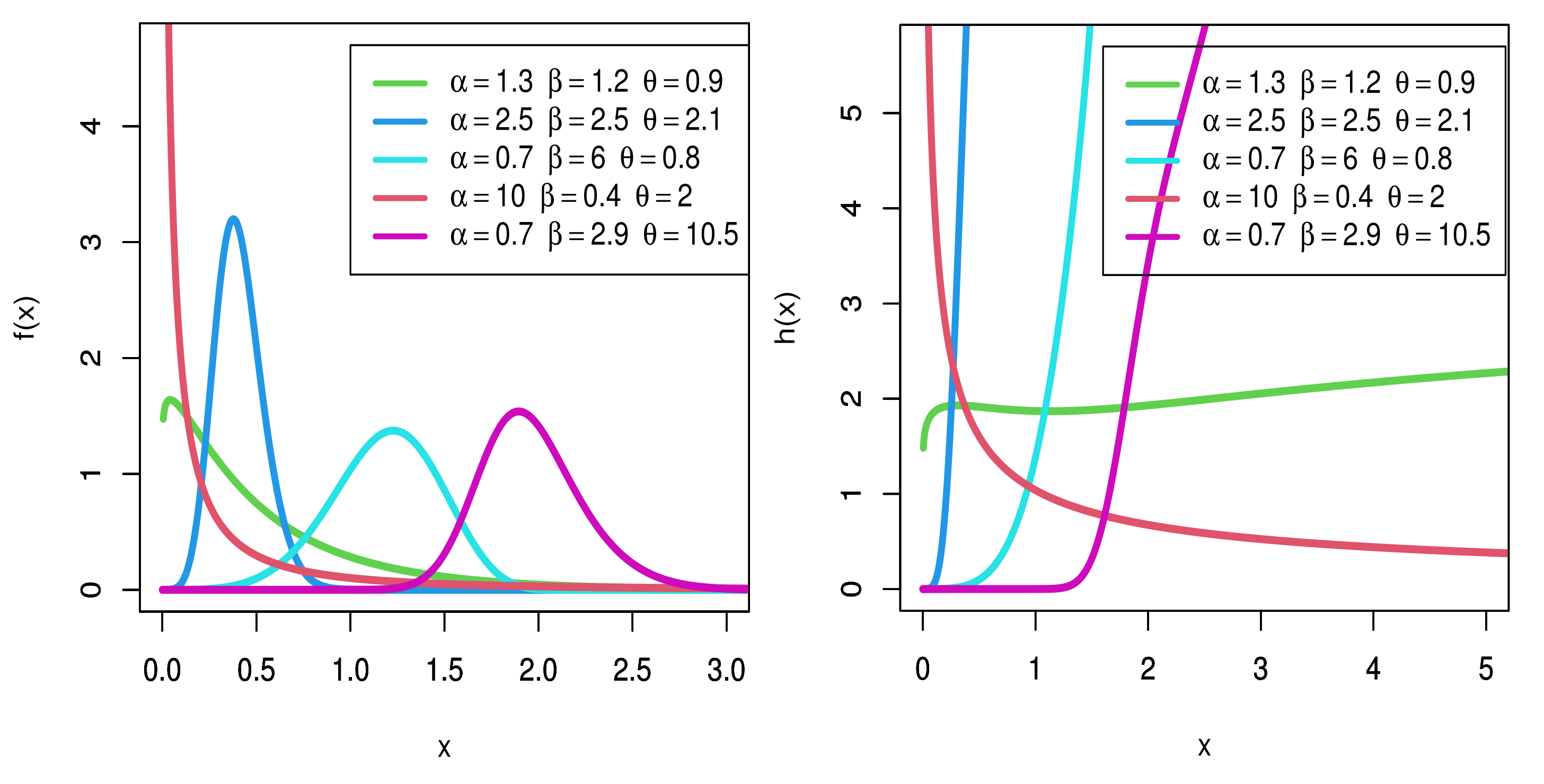
In the article under consideration, our primary focus lies in introducing a new lifetime model called the KMEW model as a new three-parameter lifetime model based on the KM transformation family, EW distribution. The following arguments give enough motivation to study the proposed model. We specify them as follows: (i) the new suggested distribution is very flexible and contains some distributions as sub-models; (ii) the shapes of the pdf for the new model can be asymmetric (unimodal, decreasing and right-skewed) and symmetric. In addition, the shapes of the hrf for the suggested model can be increasing, decreasing, constant and J-shaped; (iii) the new suggested model has a closed form for the quantile function and this makes the calculation of some properties, such as skewness and kurtosis, very easy, and generating random numbers from the new suggested model also becomes easy; (iv) some statistical and mathematical properties of the new suggested model are explored; (v) a maximum likelihood method of estimation is produced to estimate the parameters of the FB model; (vi) the KMEW is a good alternative to several lifetime distributions, such as the three-parameter exponentiated Weibull, the modified Weibull model, the Kavya–Manoharan 9 Weibull, the extended Weibull, the odd Weibull inverse Topp–Leone and the extended odd Weibull 10 inverse Nadarajah–Haghigh model for modeling skewed data in applications; (vii) we propose a bivariate SSALTs under PTIC using the KMEW model. For our proposed bivariate SSALT under PTIC, the best test plan is obtained by minimizing the asymptotic variance (AV) of the MLEs of the log of the scale parameter.

This paper is organized as follows. In Section 2, a new lifetime model using an exponentiated Weibull distribution as the baseline distribution in the KM transformation family and its different distributions are presented. In Section 3, we demonstrate the statistical features of the KMEW model. The maximum likelihood inference for model parameters is discussed in Section 4. Its application to three real datasets is discussed in Section 5. The bivariate SSALT under the PTIC model is introduced in Section 6.

2. Kavya–Manoharan Exponentiated Weibull Distribution

In this section, we construct a new flexible distribution called the Kavya–Manoharan transformation exponential Weibull (KMEW) distribution by inserting (1) into (3) to obtain

$$F_{{}_{KMEW}}(x;\alpha ,\beta ,\theta )=\frac{e}{e-1}(1-e^{-{\left[1-e^{-{\left(\alpha x\right)}^{\beta }}\right]}^{\theta }}),x>0,\alpha ,\beta ,\theta >0,$$

(6)

and the corresponding pdf is

$$f_{{}_{KMEW}}(x;\alpha ,\beta ,\theta )=\frac{e\beta \theta {\alpha }^{\beta }}{e-1}{x}^{\beta -1}{e}^{-{\left(\alpha x\right)}^{\beta }}{\left[1-e^{-{\left(\alpha x\right)}^{\beta }}\right]}^{\theta -1}{e}^{-{\left[1-e^{-{\left(\alpha x\right)}^{\beta }}\right]}^{\theta }}.$$

(7)

The survival function and hrf for the KMEW distribution are

$${\overline{F}}_{{}_{KMEW}}(x;\alpha ,\beta ,\theta )=1-\frac{e}{e-1}(1-e^{-{\left[1-e^{-{\left(\alpha x\right)}^{\beta }}\right]}^{\theta }},$$

(8)

and

$${\xi }_{{}_{KMEW}}(x;\alpha ,\beta ,\theta )=\frac{e\beta \theta {\alpha }^{\beta }}{e-1}{\left[1-e^{-{\left(\alpha x\right)}^{\beta }}\right]}^{\theta -1}\frac{x^{\beta -1}{e}^{-{\left(\alpha x\right)}^{\beta }}{e}^{-{\left[1-e^{-{\left(\alpha x\right)}^{\beta }}\right]}^{\theta }}}{1-\frac{e}{e-1}\left(1-e^{-{\left[1-e^{-{\left(\alpha x\right)}^{\beta }}\right]}^{\theta }}\right)}.$$

(9)

The cumulative hazard rate function is given by

$$H_{{}_{KMEW}}(x;\alpha ,\beta ,\theta )=-ln\left(1-\frac{e}{e-1}(1-e^{-{\left[1-e^{-{\left(\alpha x\right)}^{\beta }}\right]}^{\theta }}\right).$$

Figure 3 shows the forms of the KMEW pdf (7) and hrf in (9) using various specific parameter settings. It demonstrates that the pdf of the KMEW distribution can be unimodal and right-skewed, with very heavy tails.

Figure 3 shows a graphical representations of the hrf of the KMEW distribution with various parameter values. Forms of the pdf include symmetric, asymmetric and reversed-J form, as shown in the left of Figure 3. Forms of the hrf include increasing, decreasing and reversed-J form, as shown in the right of Figure 3. The KMEW distribution is a very flexible model that provides different distributions when its parameters are changed. It contains the following special models:

• When $\theta =1$, we obtain KM transformation Weibull (see Kavya and Manoharan [23]);
• For $\beta =2$, we obtain KM transformation exponentiated Rayleigh (new);
• Setting $\beta =1$, we have KM transformation exponentiated exponential (new);
• When $\theta =1$ and $\beta =2$, the KMEW distribution reduces to KM Rayleigh (new);
• The case $\theta =1$ and $\beta =1$ refers to the KM transformation exponential (see Kavya and Manoharan [23]).

Using the following generalized binomial ${(1-z)}^{b-1}={\sum }_{j=0}^{\infty }{(-1)}^j\left(\genfrac{}{}{0pt}{}{b-1}{j}\right)z^j,\mid z\mid <1$, and $e^{-x}={\sum }_{i=0}^{\infty }\frac{{(-x)}^i}{i!}$, we can obtain a useful linear representation for the pdf in Equation (7) as follows:

$$f_{{}_{KMEW}}\left(x\right)=\frac{e\beta \theta {\alpha }^{\beta }}{e-1}\sum _{i,j=0}^{\infty }\frac{{(-1)}^{i+j}}{i!}\left(\genfrac{}{}{0pt}{}{\theta (i+1)-1}{j}\right)x^{\beta -1}{e}^{-(j+1){\left(\alpha x\right)}^{\beta }}.$$

(10)

3. Statistical Measures

In this section, we study the statistical measures of the KMEW distribution, including quantile function, mode, moments, probability weighted moments, order statistics and entropy.

3.1. Quantile Function

Quantile functions are used in theoretical aspects, statistical applications and Monte Carlo methods. The $p^{th}$ quantile function of KMEW distribution is given by

$$x_p=Q\left(p\right)=-\frac{1}{\alpha }log{\left\{1-{\left[-log\left(\frac{p(e-1)}{e}\right)\right]}^{\frac{1}{\theta }}\right\}}^{\frac{1}{\beta }},$$

(11)

where $p\in (0,1)$. In addition, the quantile function allows us to define several shape measures, such as skewness and kurtosis. Furthermore, the analysis of the variability of the skewness and kurtosis on the shape parameters $\alpha$, $\beta$ and $\theta$ can be investigated based on quantile measures. The median can be obtained by putting $p=0.5$ in (11) as

$$median=Q\left(0.5\right)=-\frac{1}{\alpha }log{\left\{1-{\left[-log\left(\frac{0.5(e-1)}{e}\right)\right]}^{\frac{1}{\theta }}\right\}}^{\frac{1}{\beta }}.$$

3.2. Mode

The mode of the KMEW ($\alpha ,\beta ,\theta$) can be obtained as a solution of the following non-linear equation $\frac{d}{dx}log\left(f\left(x;\alpha ,\beta ,\theta \right)\right)=0$ as

$$\frac{\beta -1}{x}-\beta {\alpha }^{\beta }{x}^{\beta -1}\left(1-\frac{\theta -1}{e^{{\left(\alpha x\right)}^{\beta }}-1}+\theta e^{-{\left(\alpha x\right)}^{\beta }}{\left[1-e^{-{\left(\alpha x\right)}^{\beta }}\right]}^{\theta -1}\right)=0.$$

It is not possible to obtain the explicit solution in the general case. It has to be obtained numerically.

3.3. Moments

Statistical moments of different orders are important in defining uncertainty characteristics of the distributions. Using the expansion (10), the $r^{th}$ moment of X is attained as

$${\mu }_r^{{}^{\prime }}={\int }_0^{\infty }{x}^{r}f\left(x\right)dx=\frac{e\beta \theta {\alpha }^{\beta }}{e-1}\sum _{i,j=0}^{\infty }\frac{{(-1)}^{i+j}}{i!}\left(\genfrac{}{}{0pt}{}{\theta (i+1)-1}{j}\right){\int }_0^{\infty }{x}^{r+\beta -1}{e}^{-(j+1){\left(\alpha x\right)}^{\beta }}dx,$$

Setting $y=(j+1){\left(\alpha x\right)}^{\beta }$, after some algebra, the $r^{th}$ moment is provided via

$${\mu }_r^{{}^{\prime }}=\frac{e\theta }{(e-1){\alpha }^r}\sum _{i,j=0}^{\infty }\frac{{(-1)}^{i+j}}{i!}\left(\genfrac{}{}{0pt}{}{\theta (i+1)-1}{j}\right)\frac{\Gamma (\frac{r}{\beta }+1)}{{(j+1)}^{\frac{r}{\beta }+1}}.$$

(12)

Table A1 shows the numerical values of the $E\left(X\right)$, $E\left(X^2\right)$, $E\left(X^3\right)$, $E\left(X^4\right)$, mode, Var (X), skewness (SK) and coefficient of variation (CV) of the KMEW distribution.

The $s^{th}$ incomplete moment of KMEW distribution can be written as

$$\begin{array}{cc}\hfill {\nu }_s\left(t\right)=& E(X^s\mid X<t)={\int }_0^t{x}^{s}f\left(x\right)dx\hfill \\ \hfill & =\frac{e\theta }{(e-1){\alpha }^s}\sum _{i,j=0}^{\infty }\frac{{(-1)}^{i+j}}{i!}\left(\genfrac{}{}{0pt}{}{\theta (i+1)-1}{j}\right)\frac{\gamma (\frac{s}{\beta }+1,(j+1){\left(\alpha t\right)}^{\beta })}{{(j+1)}^{\frac{s}{\beta }+1}},\hfill \end{array}$$

(13)

where $\gamma (s,t)={\int }_0^t{x}^{s-1}{e}^{-x}dx$ is the lower incomplete gamma function. The conditional moments KMEW distribution is defined by $E(X^s\mid X>t)$. It can be written as

$$E(X^s\mid X>t)=\frac{1}{\overline{F}\left(t\right)}{H}_s\left(x\right),$$

where

$$\begin{array}{c}\hfill H_s\left(x\right)={\int }_t^{\infty }{x}^{s}f\left(x\right)dx=\frac{e\theta }{(e-1){\alpha }^s}\sum _{i,j=0}^{\infty }\frac{{(-1)}^{i+j}}{i!}\left(\genfrac{}{}{0pt}{}{\theta (i+1)-1}{j}\right)\frac{\Gamma (\frac{s}{\beta }+1,(j+1){\left(\alpha t\right)}^{\beta })}{{(j+1)}^{\frac{s}{\beta }+1}},\end{array}$$

(14)

and $\Gamma (s,t)={\int }_t^{\infty }{x}^{s-1}{e}^{-x}dx$ is the upper incomplete gamma function. The moment-generating function of the KMEW distribution can be written as

$$\begin{array}{c}\hfill M_X\left(t\right)=E\left(e^{tX}\right)={\int }_0^{\infty }{e}^{tx}f\left(x\right)dx=\sum _{r=0}^{\infty }\frac{t^r}{r!}{\mu }_r^{{}^{\prime }}\\ & & \\ \hfill =\sum _{i,j=0}^{\infty }\sum _{r=0}^{\infty }\frac{t^r}{r!}\frac{e\theta }{(e-1){\alpha }^r}\frac{{(-1)}^{i+j}}{i!}\left(\genfrac{}{}{0pt}{}{\theta (i+1)-1}{j}\right)\frac{\Gamma (\frac{r}{\beta }+1)}{{(j+1)}^{\frac{r}{\beta }+1}}.\end{array}$$

The $r^{th}$ moment of the residual lifetime is provided via

$${\mu }_{{}_{RL}}\left(t\right)=E({(X-t)}^r\mid X>t)=\frac{1}{\overline{F}\left(t\right)}{\int }_t^{\infty }{(x-t)}^{r}f\left(x\right)dx,r\ge 1.$$

(15)

Adding (10) and the binomial expansion of ${(x-t)}^r$ to the previous calculation yields

$$\begin{array}{cc}\hfill {\mu }_{{}_{RL}}\left(t\right)=& \frac{1}{\overline{F}\left(t\right)}\sum _{d=0}^r{(-t)}^{r-d}\left(\genfrac{}{}{0pt}{}{r}{d}\right){\int }_t^{\infty }{x}^{d}f\left(x\right)dx\hfill \\ \hfill & =\frac{e\theta }{\overline{F}\left(t\right)(e-1){\alpha }^d}\sum _{d=0}^r{(-t)}^{r-d}\left(\genfrac{}{}{0pt}{}{r}{d}\right)\hfill \\ \hfill & \times \sum _{i,j=0}^{\infty }\frac{{(-1)}^{i+j}}{i!}\left(\genfrac{}{}{0pt}{}{\theta (i+1)-1}{j}\right)\frac{\Gamma (\frac{d}{\beta }+1,(j+1){\left(\alpha t\right)}^{\beta })}{{(j+1)}^{\frac{d}{\beta }+1}}.\hfill \end{array}$$

(16)

Similarly, the $r^{th}$ moment of the reversed residual life may be determined utilizing method

$$m_{{}_{PL}}\left(t\right)=E({(t-X)}^r\mid X\le t)=\frac{1}{F\left(t\right)}{\int }_0^t{(t-x)}^{r}f\left(x\right)dx.$$

Adding (10) and the binomial expansion of ${(x-t)}^r$ to the previous calculation yields

$$\begin{array}{cc}\hfill m_{{}_{PL}}\left(t\right)=& \frac{1}{F\left(t\right)}\sum _{d=0}^r{(-t)}^{r-d}\left(\genfrac{}{}{0pt}{}{r}{d}\right){\int }_0^t{x}^{d}f\left(x\right)dx\hfill \\ & =\frac{e\theta }{F\left(t\right)(e-1){\alpha }^d}\sum _{d=0}^r{(-t)}^{r-d}\left(\genfrac{}{}{0pt}{}{r}{d}\right)\hfill \\ \hfill & \times \sum _{i,j=0}^{\infty }\frac{{(-1)}^{i+j}}{i!}\left(\genfrac{}{}{0pt}{}{\theta (i+1)-1}{j}\right)\frac{\gamma (\frac{d}{\beta }+1,(j+1){\left(\alpha t\right)}^{\beta })}{{(j+1)}^{\frac{d}{\beta }+1}}.\hfill \end{array}$$

(17)

The mean past (inactivity) time is denoted by

$$\begin{array}{cc}\hfill m\left(t\right)=& E((X-t)\mid X<t)=t-\frac{1}{F\left(t\right)}{\nu }_1\left(t\right)\hfill \\ & =t-\frac{e\theta }{F\left(t\right)(e-1)\alpha }\sum _{i,j=0}^{\infty }\frac{{(-1)}^{i+j}}{i!}\left(\genfrac{}{}{0pt}{}{\theta (i+1)-1}{j}\right)\frac{\gamma (\frac{1}{\beta }+1,(j+1){\left(\alpha t\right)}^{\beta })}{{(j+1)}^{\frac{1}{\beta }+1}}.\hfill \end{array}$$

(18)

3.4. Probability Weighted Moments

The probability weighted moments (PWMs) of random variable X whose Cdf is $F\left(x\right)$, say ${\xi }_{r,s}$, is provided via

$${\xi }_{r,s}=E\left(x^r{F}^{{}^s}\left(x\right)f\left(x\right)\right)={\int }_0^{\infty }{x}^r{F}^{{}^s}\left(x\right)f\left(x\right)dx.$$

Combining Equations (6) and (7), we may compute

$$F^{{}^s}\left(x\right)f\left(x\right)=\sum _{i,j,k=0}^{\infty }{\varpi }_{i,j,k}{x}^{\beta -1}{e}^{-(k+1){(\alpha x)}^{\beta }},$$

where

$${\varpi }_{i,j,k}={\left(\frac{e}{e-1}\right)}^{s+1}\frac{\beta \theta {\alpha }^{\beta }{(-1)}^{i+j+k}{(s+1)}^j}{j!}\left(\genfrac{}{}{0pt}{}{s}{j}\right)\left(\genfrac{}{}{0pt}{}{\theta (j+1)-1}{k}\right).$$

Thus, the ${(r,s)}^{th}$ PWMs of X can indeed be expressed simply by

$${\xi }_{r,s}=E\left(x^r{F}^{{}^s}\left(x\right)f\left(x\right)\right)=\sum _{i,j,k=0}^{\infty }{\varpi }_{i,j,k}\frac{\Gamma (\frac{r}{\beta }+1)}{\beta {\alpha }^{r+\beta }{(k+1)}^{\frac{r}{\beta }+1}}.$$

3.5. Order Statistics

Moments of order statistics (OS) (see [48]) are very useful in quality control and reliability when the prediction of the hazard of failure of future items depends on the times of few early failures. Assume that $X_{(1:n)}\le$⋯$\le X_{(n:n)}$ denotes the OS of a random sample $X_1,\dots ,X_n$ from a continuous population with cdf $F\left(x\right)$ and pdf $f\left(x\right)$; then, the pdf of $k^{th}$ OS, denoted by $X_{k:n}$, is provided with

$$f_{k:n}\left(x\right)=\frac{n!}{(k-1)!(n-k)!}f\left(x\right){\left(F\left(x\right)\right)}^{k-1}{\left[1-F\left(x\right)\right]}^{n-k}.$$

The pdf of the $k^{th}$ OS for KMEW distribution can be written as

$$f_{k:n}\left(x\right)=\sum _{i,j=0}^{\infty }\sum _{m=0}^{n-k}{\varphi }_{i,j,m}{f}_{Ew}(x;\alpha ,\beta ,\theta (j+1)),$$

(19)

where

$${\varphi }_{i,j,m}=\frac{n!}{(k-1)!(n-k)!}\frac{{(-1)}^{i+j+k}{(i+1)}^j\Gamma (k+m)}{i!(j+1)!\Gamma (k+m-i)}\left(\genfrac{}{}{0pt}{}{n-k}{m}\right),$$

and $f_{Ew}(x;\alpha ,\beta ,\theta (j+1))$ is an EW pdf with parameters $\alpha ,\beta$ and $\theta (j+1)$.Therefore, the pdf of the KMEW OS can be expressed as a linear combination of the EW densities. Thus, according to (19), we can find some mathematical properties of $X_{k:n}$ from those properties of EW. The $r_{th}$ moment of $X_{k:n}$ is provided via

$$E\left(X_{k:n}^r\right)=\sum _{i,j=0}^{\infty }\sum _{m=0}^{n-k}{\varphi }_{i,j,m}E\left(Z_{\theta (j+1)}^{{}^r}\right),$$

where $Z_{\theta (j+1)}^{{}^r}$ has EW distribution with parameters $\alpha ,\beta$ and $\theta (j+1)$.

3.6. Entropy

The entropy of a random variable X is a measure of variation of uncertainty and has been used in many fields, such as physics, engineering and economics. The Rényi entropy [49] is characterized by

$$I_{{}_R}(\zeta )=\frac{1}{1-\zeta }log\left[{\int }_0^{\infty }f{}^{\zeta }\left(x\right)dx\right],\zeta >0,\zeta \ne 1.$$

From (7), the Rényi entropy of X can be obtained as follows:

$$I_{{}_R}(\zeta )=\frac{1}{1-\zeta }log\left\{{\left(\frac{e\beta \theta {\alpha }^{\beta }}{e-1}\right)}^{\zeta }{\int }_0^{\infty }{x}^{\zeta (\beta -1)}{e}^{-\zeta {\left(\alpha x\right)}^{\beta }}{\left[1-e^{-{\left(\alpha x\right)}^{\beta }}\right]}^{\zeta (\theta -1)}{e}^{-\zeta {\left[1-e^{-{\left(\alpha x\right)}^{\beta }}\right]}^{\theta }}dx\right\},$$

using power series, and, after some simplifications, we obtain

$$I_{{}_R}(\zeta )=\frac{1}{1-\zeta }log\left\{{\left(\frac{e\beta \theta {\alpha }^{\beta }}{e-1}\right)}^{\zeta }\sum _{i,j=0}^{\infty }\frac{{(-1)}^{i+j}{\zeta }^i}{i!{\alpha }^{\zeta (\beta -1)+1}}\left(\genfrac{}{}{0pt}{}{\theta (\zeta +i)-\zeta }{j}\right)\frac{\Gamma (\zeta +\frac{1}{\beta }(1-\zeta ))}{{\left(\zeta +j\right)}^{\zeta +\frac{1}{\beta }(1-\zeta )}}\right\}.$$

4. Maximum Likelihood Estimation

In this section, we use maximum likelihood (see [50]) to estimate the parameters of the KMEW distribution. Let $x_1,\dots ,x_n$ be a random sample of size n from the KMEW distribution given by (7). The log- likelihood function (log-LLF) of the KMEW distribution is provided via

$$\begin{array}{cc}\hfill L=& nlog\left(\frac{e}{e-1}\right)+nlog(\beta )+nlog(\theta )+n\beta log\alpha -\sum _{i=1}^n{\left[A_i\right]}^{\theta }\hfill \\ \hfill & +(\beta -1)\sum _{i=1}^{n}log\left(x_i\right)-\sum _{i=1}^n{\left(\alpha x_i\right)}^{\beta }+\left(\theta -1\right)\sum _{i=1}^{n}log\left[A_i\right].\hfill \end{array}$$

(20)

In order to obtain the MLEs of parameters $\alpha ,\beta$ and $\theta$, we compute the first partial derivatives of (20) with respect to $\alpha ,\beta$ and $\theta$, and, equating them to 0, we derive the accompanying three equations as:

$$\begin{array}{cc}\hfill \frac{\partial L}{\partial \alpha }=& \frac{n\beta }{\alpha }-\beta \sum _{i=1}^n{x}_i{\left(\alpha x_i\right)}^{\beta -1}+\left(\theta -1\right)\sum _{i=1}^n\frac{B_i}{A_i}-\theta \sum _{i=1}^n{\left(A_i\right)}^{\theta -1}{B}_i,\hfill \end{array}$$

(21)

$$\begin{array}{cc}\hfill \frac{\partial L}{\partial \beta }=& \frac{n}{\beta }+nlog\alpha +\sum _{i=1}^{n}log\left(x_i\right)-\sum _{i=1}^n{\left(\alpha x_i\right)}^{\beta }log\left(\alpha x_i\right)\hfill \\ \hfill & +\left(\theta -1\right)\sum _{i=1}^n\frac{D_i}{A_i}-\theta \sum _{i=1}^n{D}_i{\left(A_i\right)}^{\theta -1},\hfill \end{array}$$

(22)

and

$$\frac{\partial L}{\partial \theta }=\frac{n}{\theta }+\sum _{i=1}^{n}log\left[A_i\right]-\sum _{i=1}^n{\left(A_i\right)}^{\theta }log\left[A_i\right].$$

(23)

Then, the MLEs of the parameters $\alpha ,\beta$ and $\theta$ are obtained by solving a non-linear system of equations $\frac{\partial L}{\partial \alpha }=0$, $\frac{\partial L}{\partial \beta }=0$ and $\frac{\partial L}{\partial \theta }=0$. The MLEs can be evaluated numerically using statistical software. For interval estimation on the model parameters, we require the observed information matrix

$$J\left(\Theta \right)=\left(\begin{array}{ccc}{U}_{\alpha \alpha }& U_{\alpha \beta }& U_{\alpha \theta }\\ U_{\alpha \beta }& U_{\beta \beta }& U_{\beta \theta }\\ U_{\alpha \theta }& U_{\beta \theta }& U_{\theta \theta }\end{array}\right),$$

whose elements are

$$\begin{array}{c}{U}_{\alpha \alpha }=\frac{{\partial }^{2}L}{\partial {\alpha }^2}=-\frac{n\beta }{{\alpha }^2}-\theta {\displaystyle \sum _{i=1}^n}{\left(A_i\right)}^{\theta -2}\left(\left(\theta -1\right){\left(B_i\right)}^2+A_i{C}_i\right)+\beta \left(\beta -1\right){\alpha }^{\beta -2}{\displaystyle \sum _{i=1}^n}{\left(x_i\right)}^{\beta }\hfill \\ +\left(\theta -1\right){\displaystyle \sum _{i=1}^n}\frac{C_i{A}_i-{\left(B_i\right)}^2}{{\displaystyle \sum _{i=1}^n}{\left(A_i\right)}^2},\hfill \end{array}$$

$$\begin{array}{c}{U}_{\alpha \beta }=\frac{{\partial }^{2}L}{\partial \alpha \partial \beta }=\frac{n}{\alpha }-\theta {\displaystyle \sum _{i=1}^n}{\left(A_i\right)}^{\theta -2}\left(\left(\theta -1\right)D_i{B}_i+A_i{F}_i\right)+{\alpha }^{\beta -1}{\displaystyle \sum _{i=1}^n}{\left(x_i\right)}^{\beta }\hfill \\ +\beta {\alpha }^{\beta -1}log\left[\alpha \right]{\displaystyle \sum _{i=1}^n}{\left(x_i\right)}^{\beta }+\beta {\alpha }^{\beta -1}{\displaystyle \sum _{i=1}^n}{\left(x_i\right)}^{\beta }log\left[x_i\right]+\left(\theta -1\right){\displaystyle \sum _{i=1}^n}\frac{F_i{A}_i-D_i{B}_i}{{\displaystyle \sum _{i=1}^n}{\left(A_i\right)}^2},\hfill \end{array}$$

$$U_{\alpha \theta }=\frac{{\partial }^{2}L}{\partial \alpha \partial \theta }={\displaystyle \sum _{i=1}^n}\frac{B_i}{A_i}-{\displaystyle \sum _{i=1}^n}{B}_i{\left(A_i\right)}^{\theta -1}\left(1+\theta log\left[A_i\right]\right),$$

$$\begin{array}{c}{U}_{\beta \beta }=\frac{{\partial }^{2}L}{\partial {\beta }^2}=-\frac{n}{{\beta }^2}-\theta {\displaystyle \sum _{i=1}^n}{\left(A_i\right)}^{\theta -2}\left(\left(\theta -1\right){\left(D_i\right)}^2+A_i{E}_i\right)+{\displaystyle \sum _{i=1}^n}{{\left(\alpha x_i\right)}^{\beta }\left(log\left[\alpha x_i\right]\right)}^2\hfill \\ +\left(\theta -1\right){\displaystyle \sum _{i=1}^n}\frac{E_i{A}_i-{\left(D_i\right)}^2}{{\displaystyle \sum _{i=1}^n}{\left(A_i\right)}^2},\hfill \end{array}$$

$$U_{\beta \theta }=\frac{{\partial }^{2}L}{\partial \beta \partial \theta }={\displaystyle \sum _{i=1}^n}\frac{D_i}{A_i}-{\displaystyle \sum _{i=1}^n}{D}_i{\left(A_i\right)}^{\theta -1}\left(1+\theta log\left[A_i\right]\right),$$

and

$$U_{\theta \theta }=\frac{{\partial }^{2}L}{\partial {\theta }^2}=-\frac{n}{{\theta }^2}-{\displaystyle \sum _{i=1}^n}{\left(A_i\right)}^{\theta }{\left(log\left[A_i\right]\right)}^2,$$

where

$$A_i=1-e^{-{\left(\alpha x_i\right)}^{\beta }},$$

$$B_i=\frac{\partial A_i}{\partial \alpha }=\beta x_i{\left(\alpha x_i\right)}^{\beta -1}{e}^{-{\left(\alpha x_i\right)}^{\beta }}=\beta x_i{\left(\alpha x_i\right)}^{\beta -1}\left(1-A_i\right),$$

$$C_i=\frac{\partial B_i}{\partial \alpha }=\beta {\left(x_i\right)}^2{\left(\alpha x_i\right)}^{\beta -2}\left((\beta -1)\left(1-A_i\right)-\alpha B_i\right),$$

$$D_i=\frac{\partial A_i}{\partial \beta }={\left(\alpha x_i\right)}^{\beta }log\left(\alpha x_i\right)e^{-{\left(\alpha x_i\right)}^{\beta }}={\left(\alpha x_i\right)}^{\beta }log\left(\alpha x_i\right)\left(1-A_i\right),$$

$$E_i=\frac{\partial D_i}{\partial \beta }=log\left[\alpha x_i\right]D_i\left(1-{\left(\alpha x_i\right)}^{\beta }log\left[\alpha x_i\right]\right),$$

and

$$F_i=\frac{\partial B_i}{\partial \beta }=x_i{\left(\alpha x_i\right)}^{\beta -1}\left(1-A_i+\beta \left(1-A_i\right)log\left[\alpha x_i\right]-\beta D_i\right).$$

5. Application of Real Data

Three genuine data sets from engineering and medical science are used to demonstrate the importance and adaptability of the proposed KMEW model. We utilize the “maxLik” package to compute likelihood estimates in the R package using the Newton–Raphson (NR) algorithms; see Henningsen and Toomet [51]. The first dataset is the waiting times (in minutes) of 100 bank clients until the service is provided. It was originally used by [52]. The data are as follows: 0.8, 0.8, 19.9, 20.6, 21.3, 21.4, 21.9, 23.0, 2.1, 2.6, 2.7, 2.9, 3.1, 3.2, 3.3, 3.5, 3.6, 4.0, 4.1, 4.2, 4.2, 4.3, 4.3, 4.4, 4.4, 4.6, 6.3, 6.7, 6.9, 7.1, 7.1, 7.1, 7.1, 7.4, 7.6, 7.7, 8, 8.2, 8.6, 8.6, 8.6, 8.8, 8.8, 8.9, 8.9, 9.5, 9.6, 9.7, 9.8, 10.7, 10.9, 11, 11, 11.1, 11.2, 4.7, 4.7, 1.3, 1.5, 1.8, 1.9, 1.9, 4.8, 4.9, 4.9, 5, 5.3, 5.5, 5.7, 5.7, 6.1, 6.2, 6.2, 6.2, 11.2, 11.5, 11.9, 12.4, 12.5, 12.9, 13, 13.1, 13.3, 13.6, 13.7, 13.9, 14.1, 15.4, 15.4, 17.3, 17.3, 18.1, 18.2, 18.4, 18.9, 19, 27, 31.6, 33.1, 38.5.

The second dataset from [53] contains the time between failures of secondary reactor pumps (thousands of hours): 2.160, 0.746, 0.402, 0.954, 0.491, 6.560, 4.992, 0.347, 0.150, 0.358, 0.101, 1.359, 3.465, 1.060, 0.614, 1.921, 4.082, 0.199, 0.605, 0.273, 0.070, 0.062, 5.320. These data were used by [54] to fit a beta-flexible Weibull distribution. Looking at

Table 1. MLE with SE, KS test values and different measures of goodness of fit for waiting times data.

		Estimates	SE	AINC	BINC	CVM	AD	KS	PV
KMEW	$\alpha$	0.1173	0.0511	640.0457	647.8612	0.0174	0.1252	0.0364	0.9995
	$\beta$	1.1036	0.3339
	$\theta$	1.9522	1.0881
GW	$\alpha$	0.1905	0.1065	640.0668	647.8823	0.0175	0.1271	0.0364	0.9994
	$\beta$	0.9056	0.2570
	$\theta$	2.6750	1.6430
KMW	$\alpha$	1.5432	0.1149	640.0468	648.2572	0.0373	0.2427	0.0541	0.9316
	$\beta$	0.0754	0.0054
MW	$\alpha$	1.7405	0.2171	641.2957	649.1112	0.0310	0.1978	0.0439	0.9905
	$\beta$	−0.0225	0.0145
	$\theta$	0.0210	0.0084
EW	$\alpha$	1.4491	0.1139	643.6791	651.4946	0.0656	0.4134	0.0590	0.8767
	$\beta$	236.914	362.8947
	$\theta$	0.3595	0.3027
OWITL	$\alpha$	1.8517	0.4051	640.0527	647.8682	0.0217	0.1534	0.0411	0.995
	$\beta$	0.3721	0.5036
	$\theta$	0.5540	0.2879
EOWINH	$\alpha$	2.3481	0.9309	642.5829	653.0035	0.0218	0.1475	0.039	0.9981
	$\beta$	0.3927	0.3300
	$\theta$	62.1123	57.6765
	$\lambda$	0.2575	0.1058

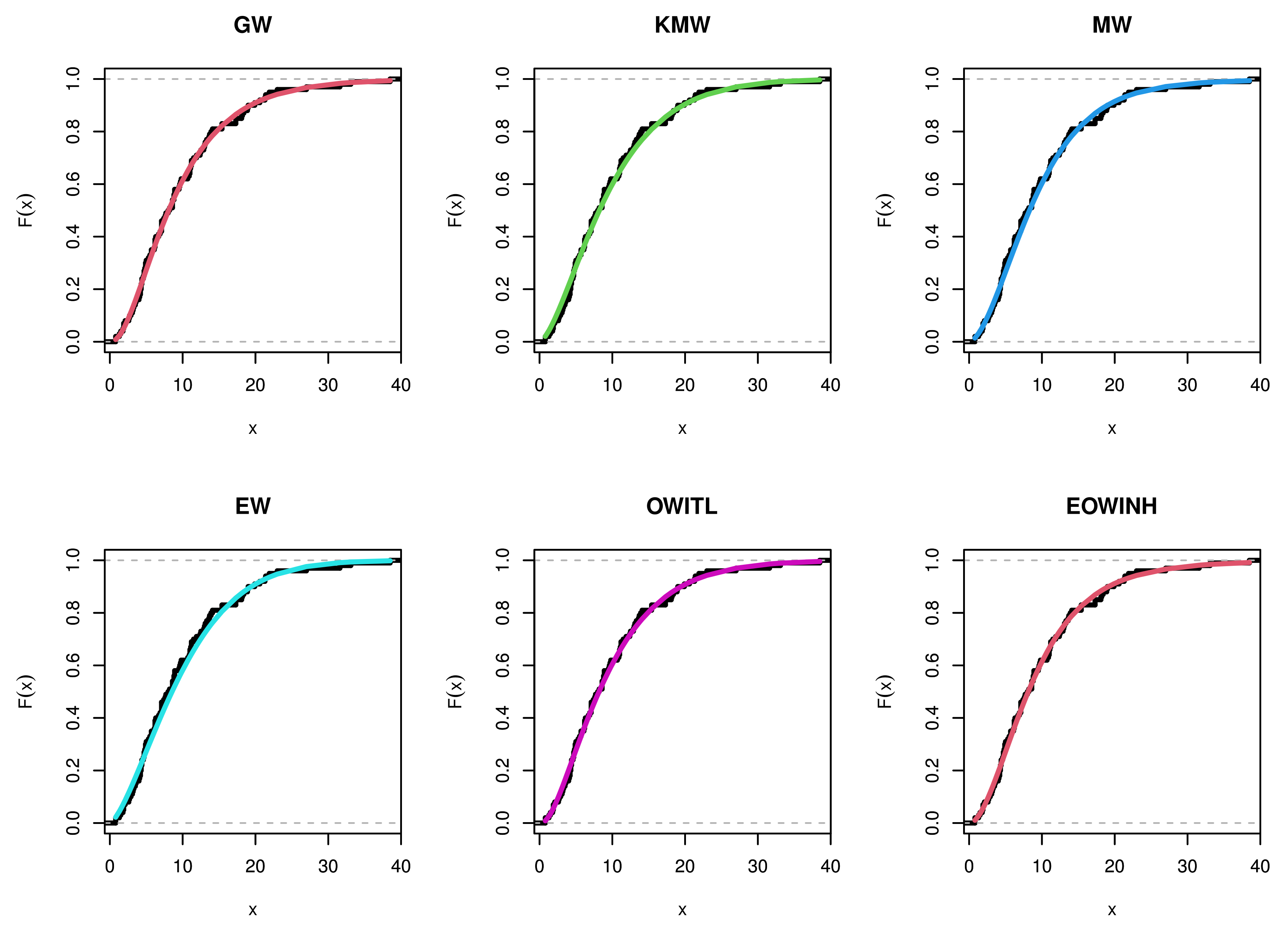
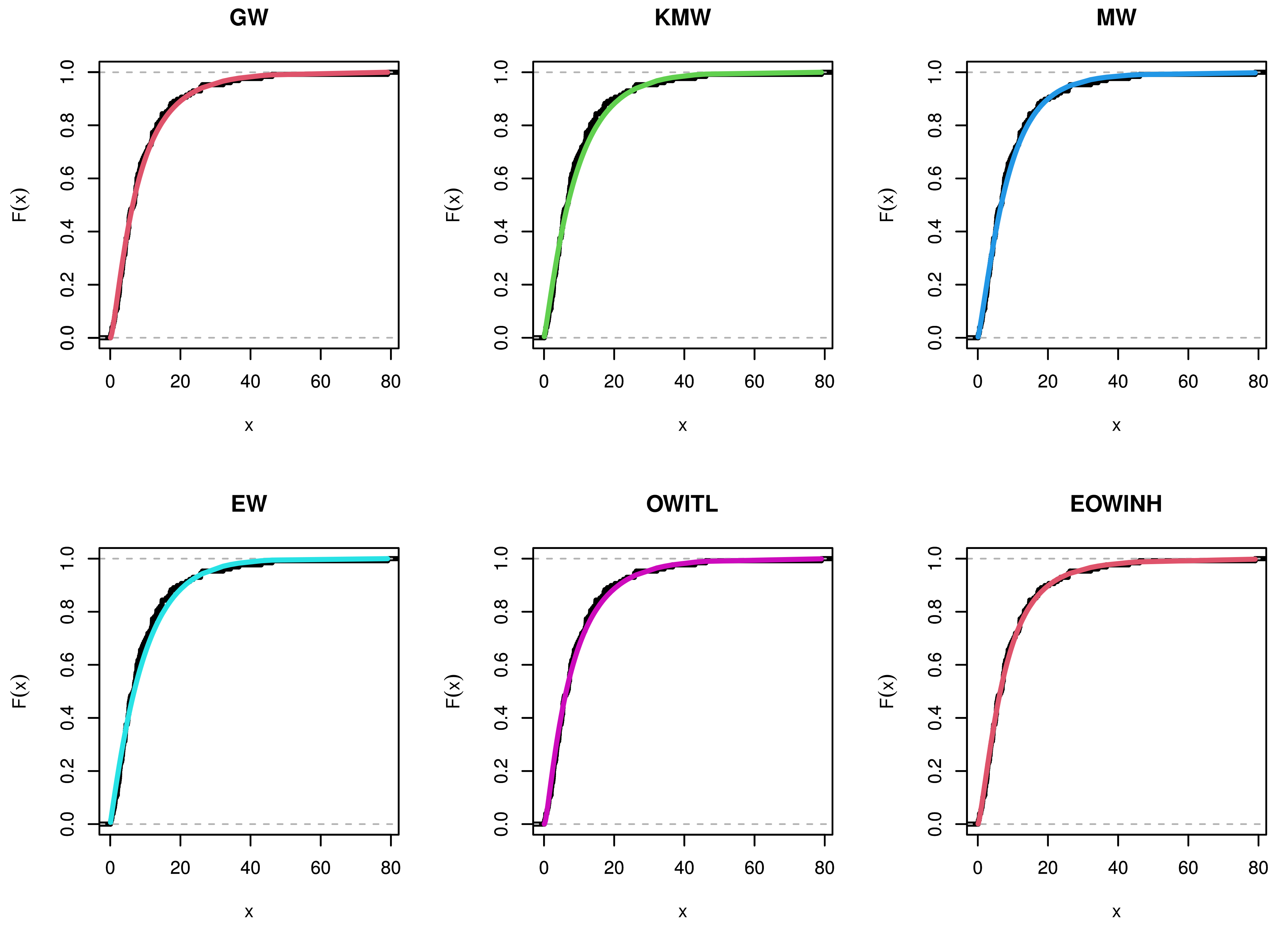
and the results in [54], we conclude that the our distribution is better than the beta-flexible Weibull distribution and many other distributions.The third dataset is remission periods (in months) of a random sample of 128 bladder cancer patients [55]. In this example, we compare the KMEW distribution with some competing distributions, such as the EW [56], modified Weibull (MW) [57], Kavya–Manoharan Weibull (KMW) [23], generalized Weibull (GW) [58], extended Weibull (ExW) [59], odd Weibull inverse Topp–Leone (OWITL) [60] and extended odd Weibull inverse Nadarajah–Haghighi (EOWINH) [61] distributions. What follows is the application of the proposed distribution to the three datasets and an observation of the findings in Table 1,

Table 2. MLE with SE, KS test values and different measures of goodness of fit for time between failures of secondary reactor pumps data.

		Estimates	SE	AINC	BINC	CVM	AD	KS	PV
KMEW	$\alpha$	0.5593	0.1505	69.6296	73.0361	0.0400	0.2902	0.0981	0.9643
	$\beta$	1.2056	0.9861
	$\theta$	1.4105	1.2381
KMW	$\alpha$	0.8879	0.1388	69.7596	73.0793	0.0551	0.3744	0.1081	0.9248
	$\beta$	0.5172	0.1356
MW	$\alpha$	0.7924	0.1925	71.0165	74.4229	0.0682	0.4442	0.1198	0.8573
	$\beta$	0.0090	0.0849
	$\theta$	0.7523	0.2198
EW	$\alpha$	0.8007	0.1454	71.0369	74.4434	0.0669	0.4381	0.1195	0.8593
	$\beta$	206.889	2104.018
	$\theta$	0.2615	0.4529
OWITL	$\alpha$	0.6178	0.4464	69.8434	73.2499	0.0432	0.2954	0.1014	0.9530
	$\beta$	1.8928	0.3974
	$\theta$	0.8714	0.3549
EOWINH	$\alpha$	2.5359	1.9491	72.8852	77.4272	0.0483	0.3438	0.1034	0.9455
	$\beta$	0.4878	1.9310
	$\theta$	89.9997	2.9563
	$\lambda$	0.1168	0.0945

and

Table 3. MLEs with SE, different criterion measures and K–S of parameters for bladder cancer.

		Estimates	SE	AINC	BINC	CVM	AD	KS	PV
KMEW	$\alpha$	0.1581	0.0718	829.5181	838.0742	0.0356	0.2421	0.0392	0.9893
	$\beta$	0.7789	0.1692
	$\theta$	2.1304	0.8784
GW	$\alpha$	0.2782	0.1521	829.9013	838.4574	0.0405	0.2708	0.0429	0.9728
	$\beta$	0.6698	0.1375
	$\theta$	2.6633	1.1856
KMW	$\alpha$	1.1584	0.0728	831.7673	838.4713	0.0824	0.5150	0.0605	0.7374
	$\beta$	0.0785	0.0066
MW	$\alpha$	1.2315	0.0968	830.3780	838.9341	0.0459	0.2816	0.0480	0.9295
	$\beta$	−0.0118	0.0036
	$\theta$	0.0727	0.0169
EW	$\alpha$	1.0530	0.0689	836.1976	844.7537	0.1164	0.7103	0.0662	0.6295
	$\beta$	368,598.718	2.6641
	$\theta$	0.1812	0.1273
OWITL	$\alpha$	1.2459	0.2442	832.5163	841.0724	0.0660	0.4406	0.0520	0.8797
	$\beta$	0.4881	0.3990
	$\theta$	0.6159	0.2797
EOWINH	$\alpha$	2.2456	1.1872	830.7619	842.1700	0.0403	0.2702	0.0422	0.9768
	$\beta$	0.4988	0.2580
	$\theta$	99.9987	156.6841
	$\lambda$	0.1965	0.1089

, which show standard errors (SEs), Akaike information criterion (AINC), Bayesian information criterion (BINC), Cramér–von-Mises (CVM) [62,63], Kolmogorov–Smirnov (KS) [64,65] with its p-value (PV) and Anderson–Darling (AD) [66,67]. We find that our proposed distribution is the best model because it has the lowest values for all measurements except PV. Although the PV of KMEW is equal to the GW distribution, KMEW is better than GW because the values of AINC, BINC, CVM and AD for KMEW distribution are smaller than the values of GW. The best model is the one that has the smallest values of AINC, BINC, CVM, AD and KS, and the largest value of PV.

For waiting times data, we discussed Figure 4, Figure 5, Figure 6, Figure 7 and Figure 8. For time between failures of secondary reactor pumps data, we discussed Figure 9, Figure 10, Figure 11, Figure 12 and Figure 13. For bladder cancer data, we discussed Figure 14, Figure 15, Figure 16, Figure 17 and Figure 18.

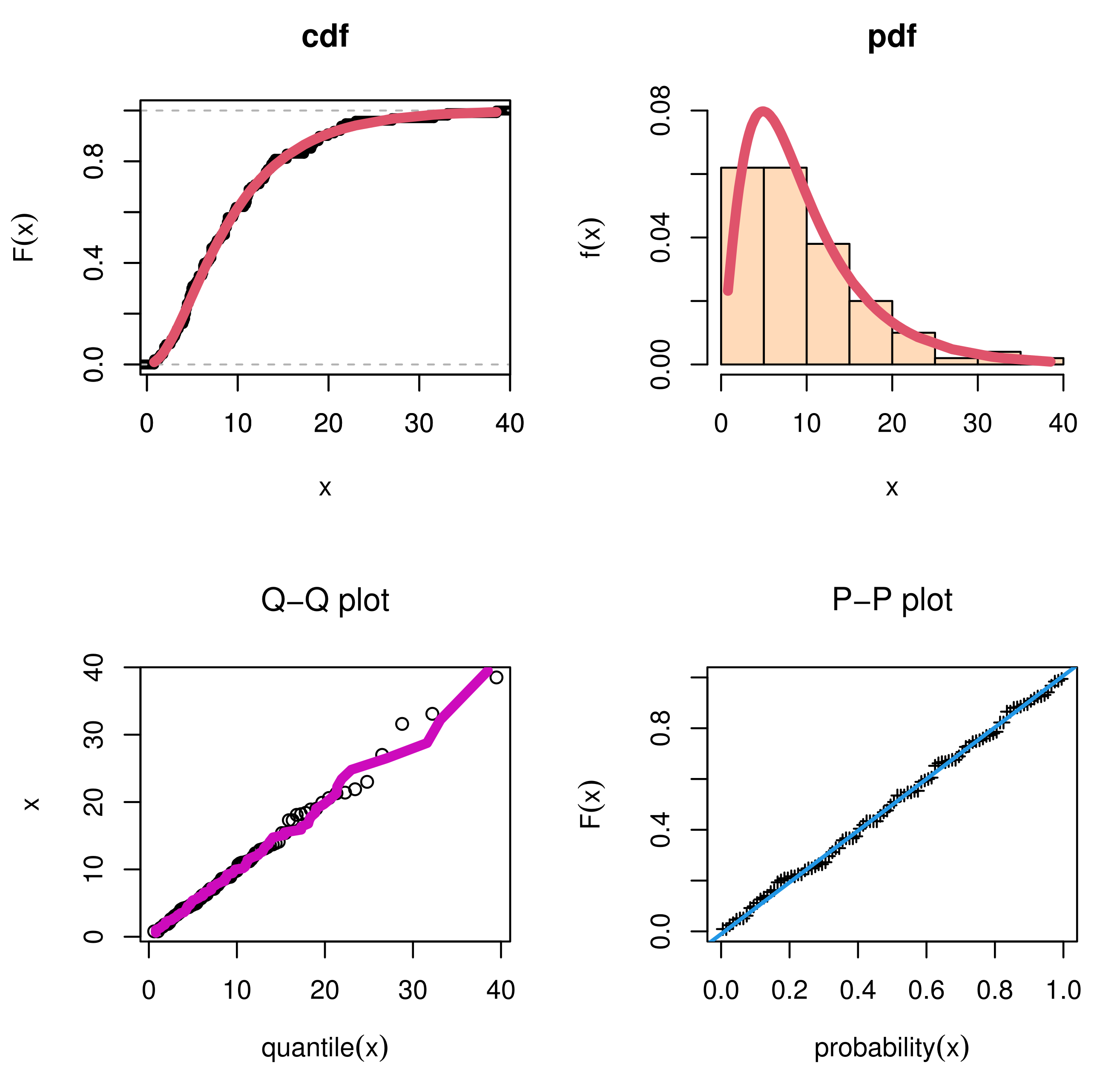
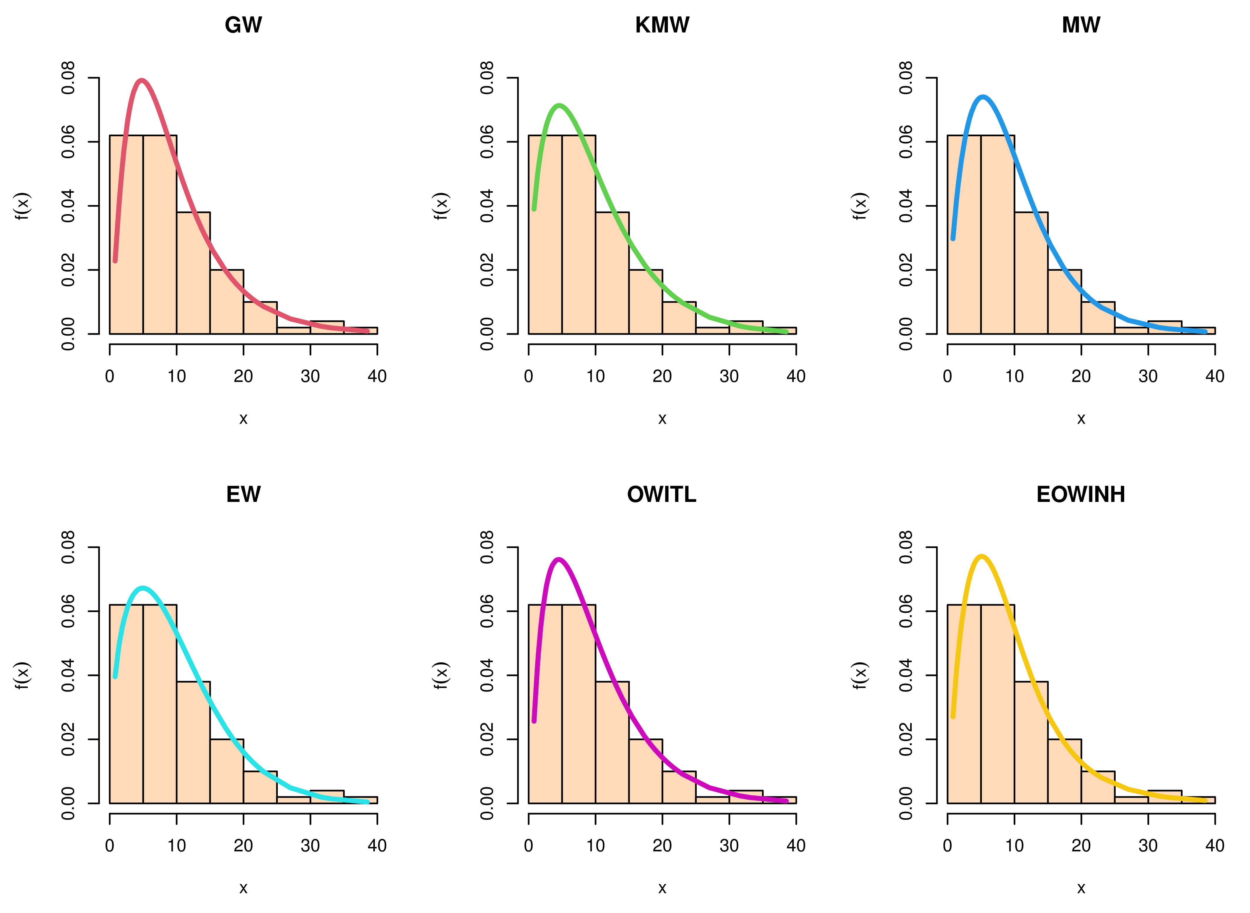
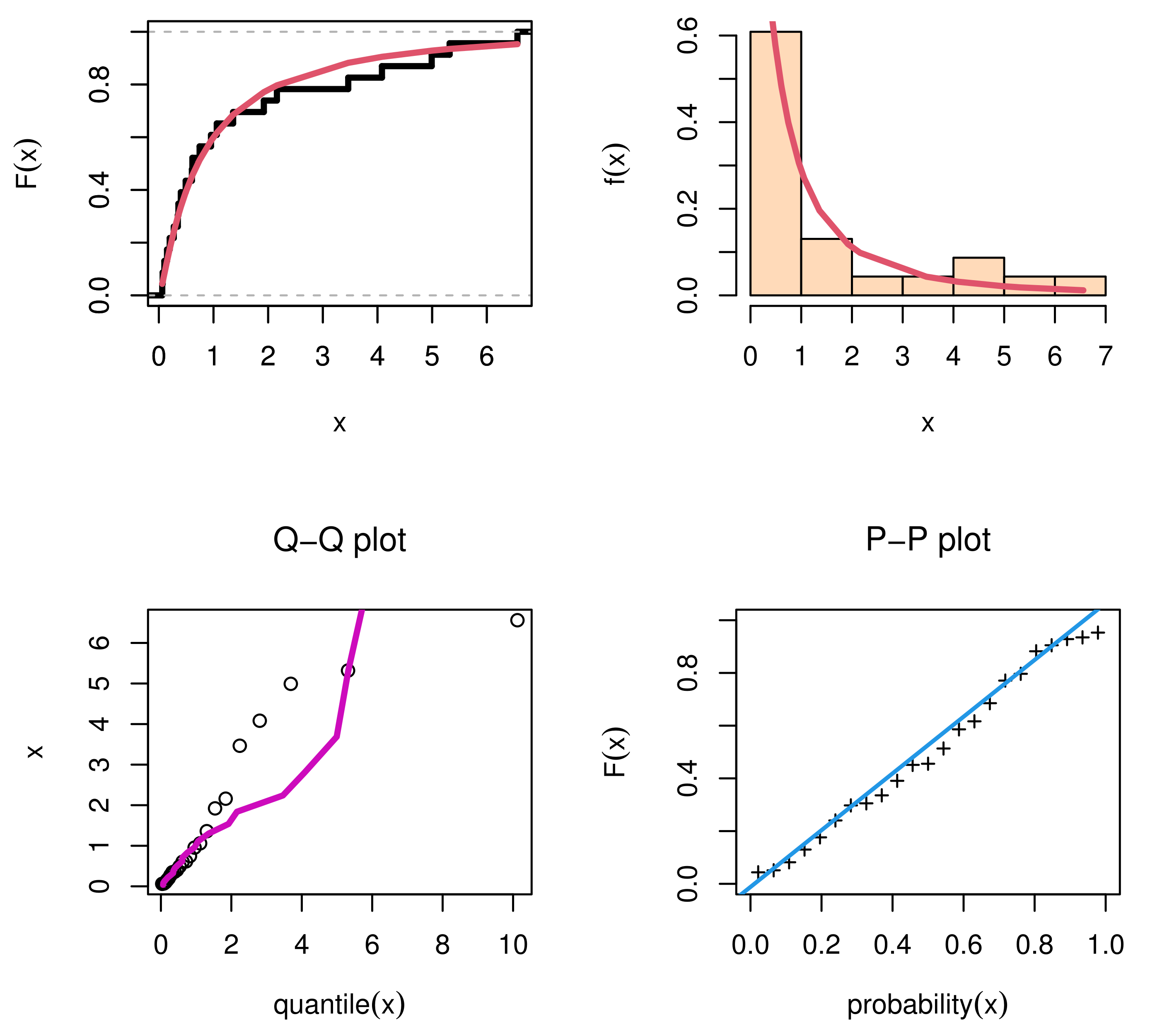
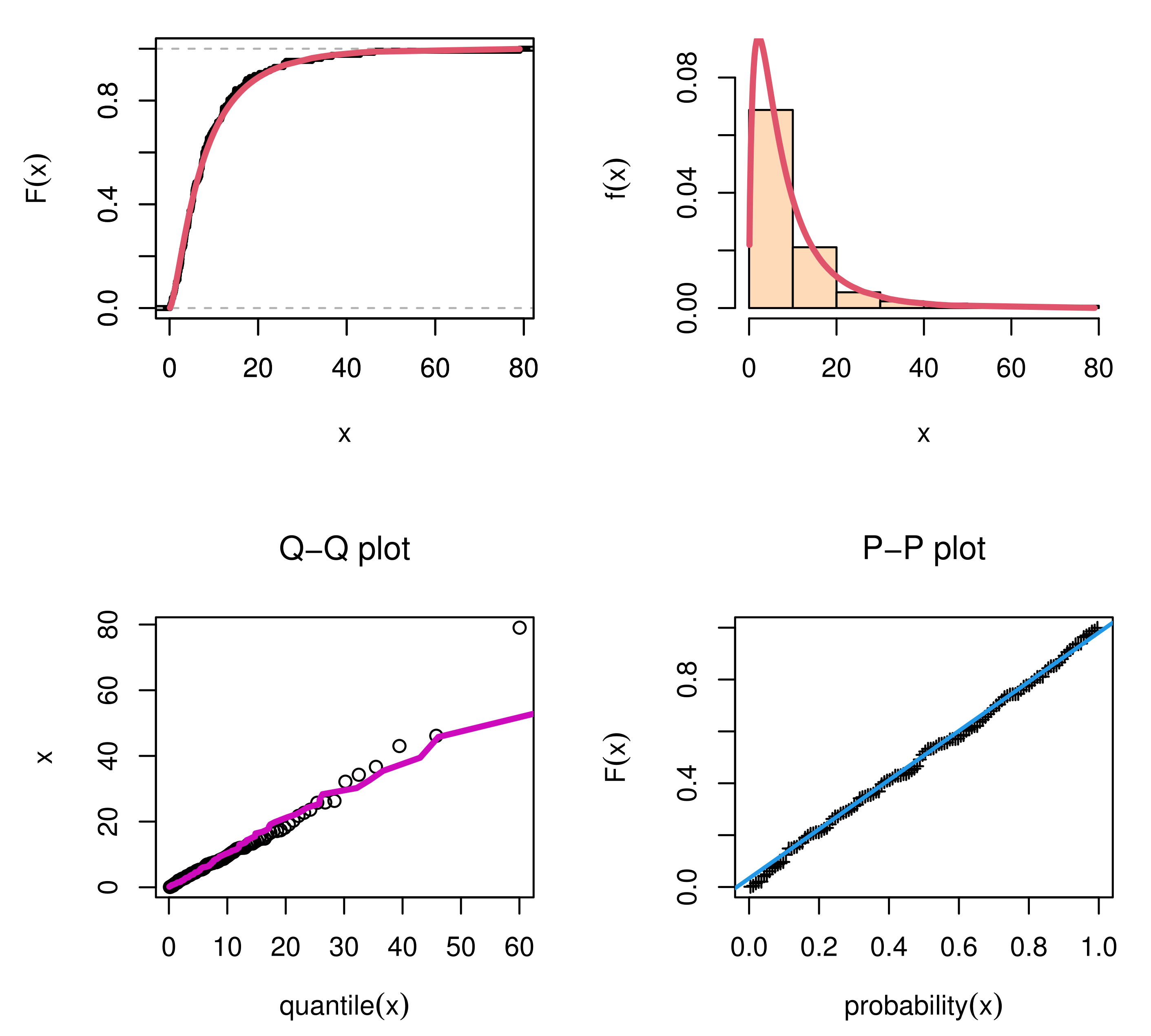
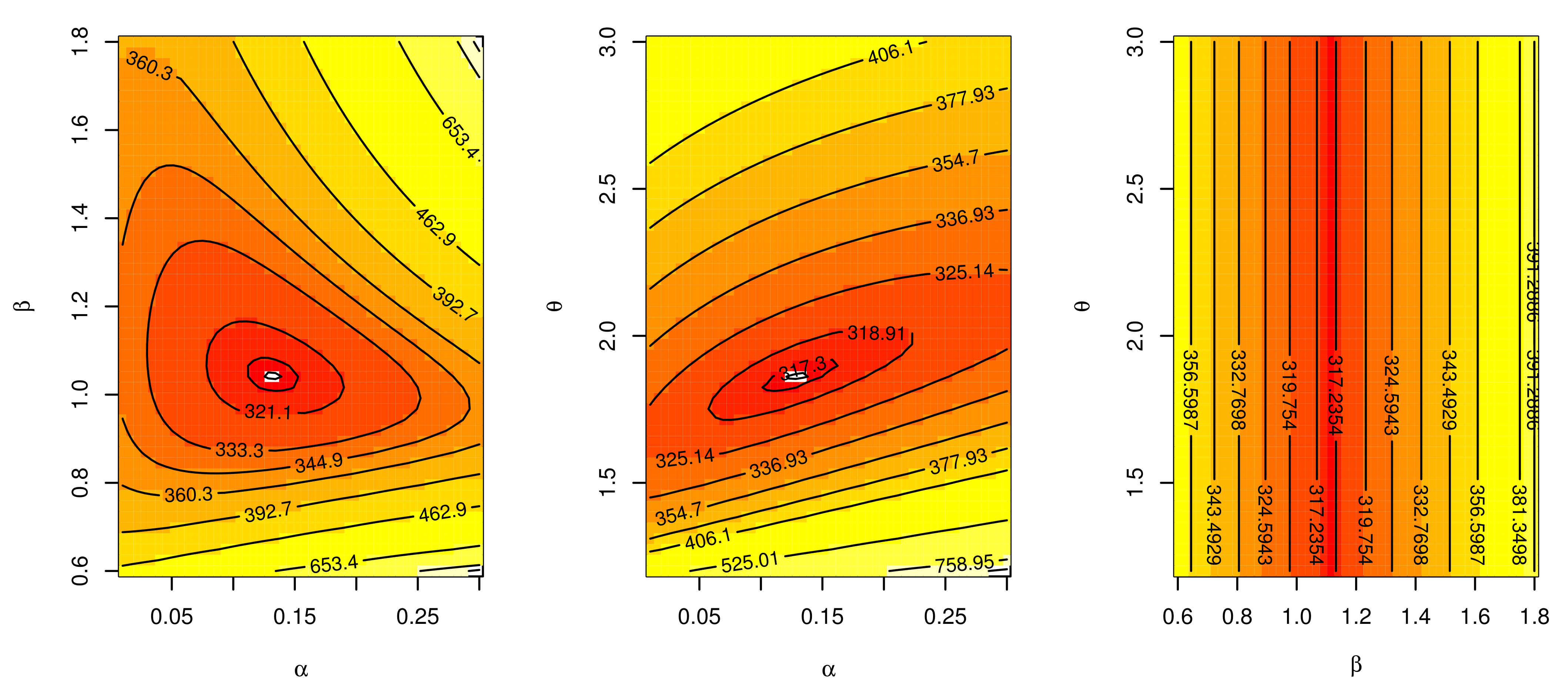
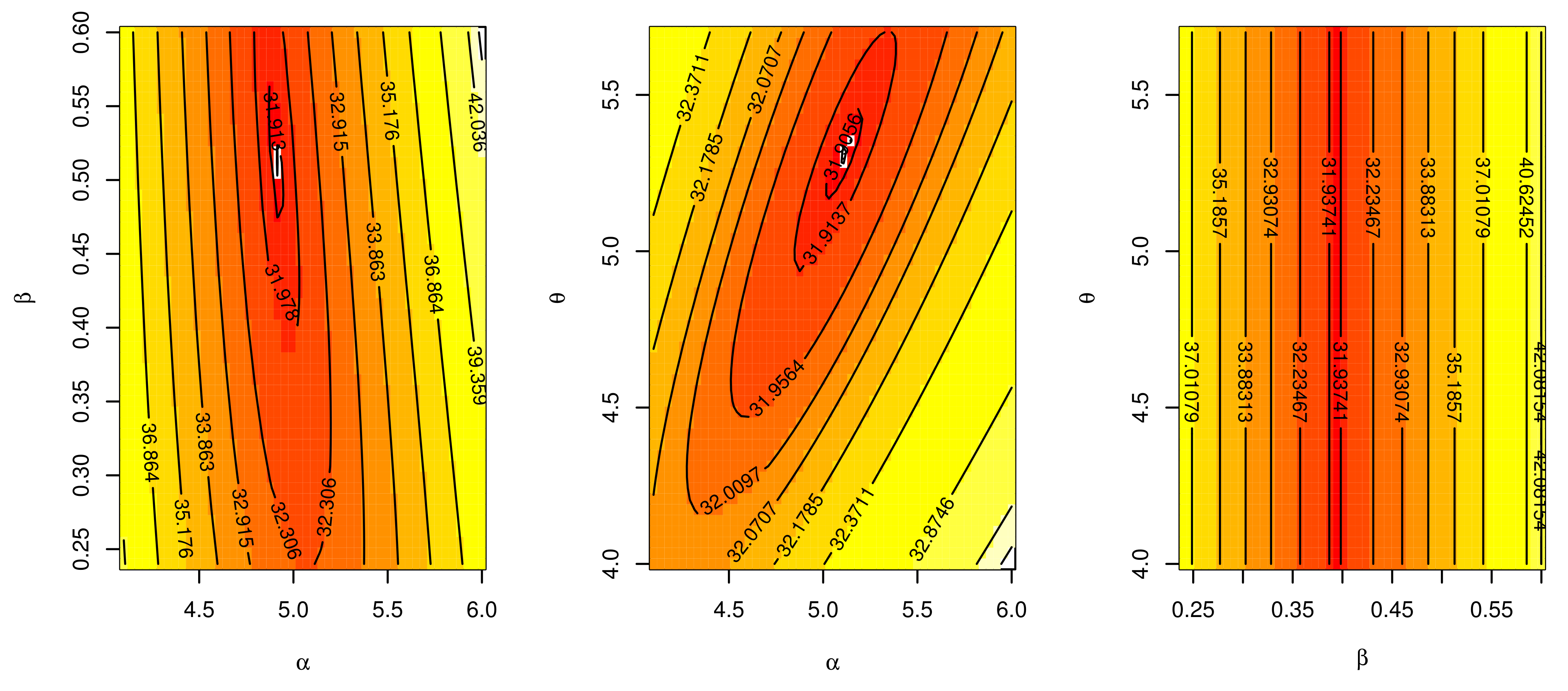
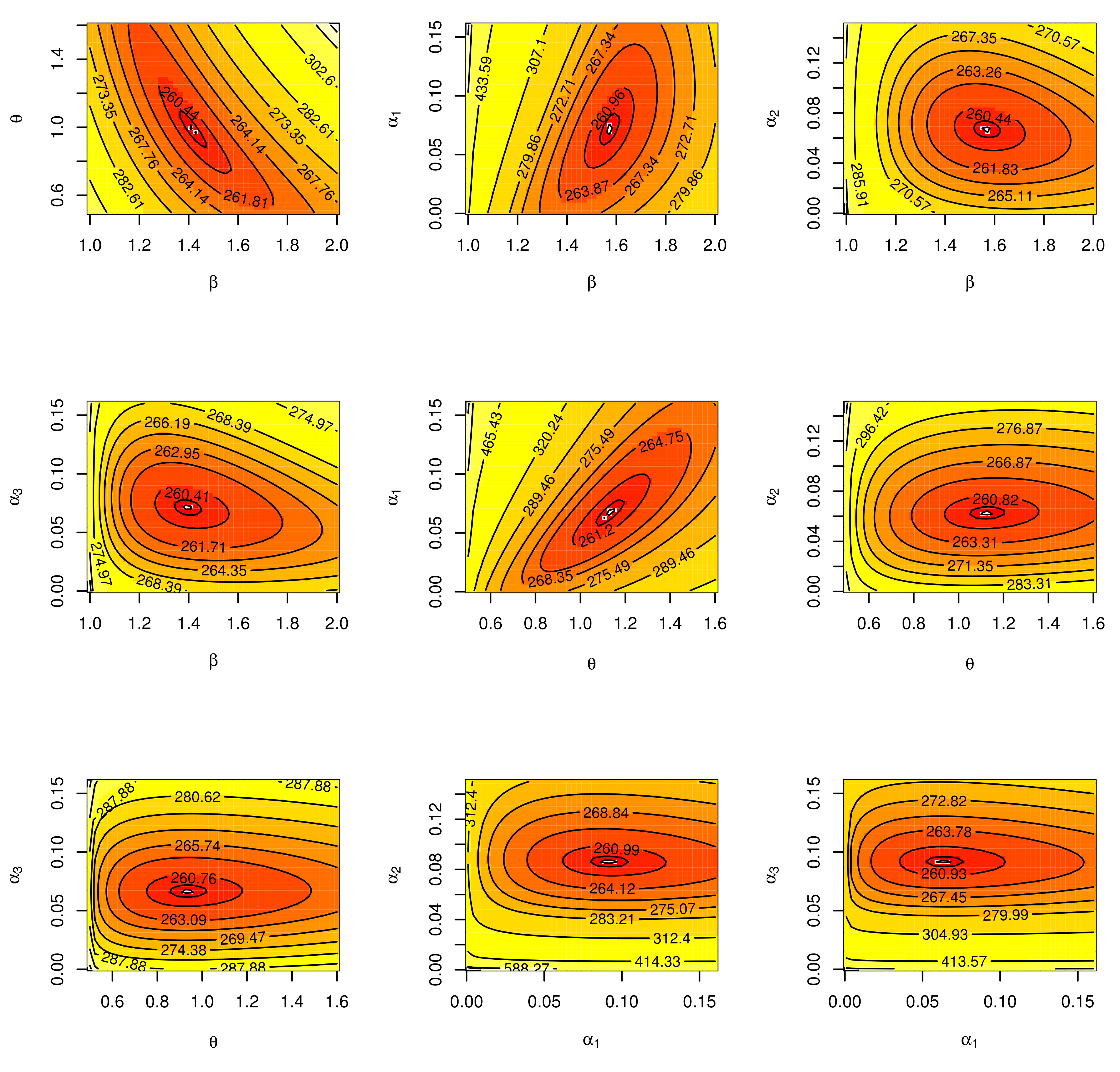
Figure 5, Figure 10 and Figure 15 support this result, demonstrating that the estimated pdf is close to the probability histogram and the calculated cdf is close to the actual cdf. We sketched the log-likelihood for every pair of parameters, while fixing the other parameters, as shown in Figure 8, Figure 13 and Figure 18. We plot cdf and pdf of alternative models in Figure 6, Figure 7, Figure 11, Figure 12, Figure 16, and Figure 17 for the three real data sets.. We find that the root of the parameter pair is a single point, which assures that the roots are unique. 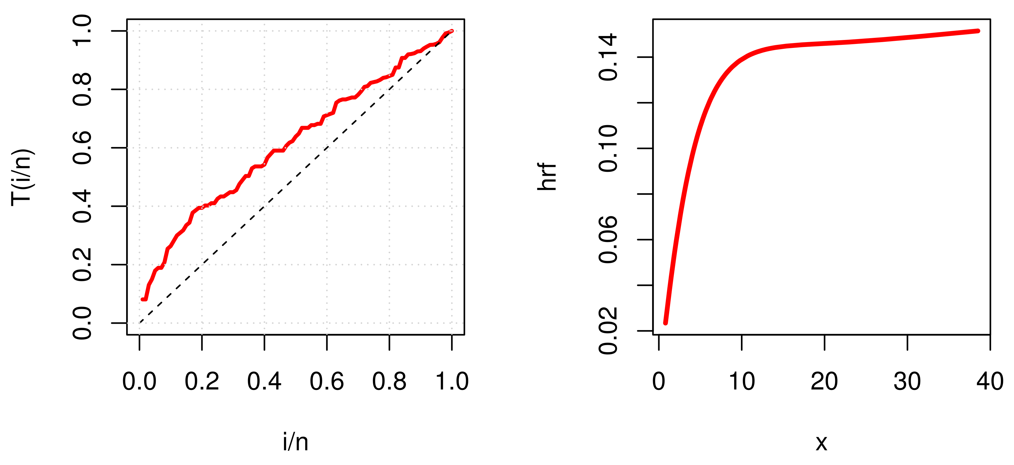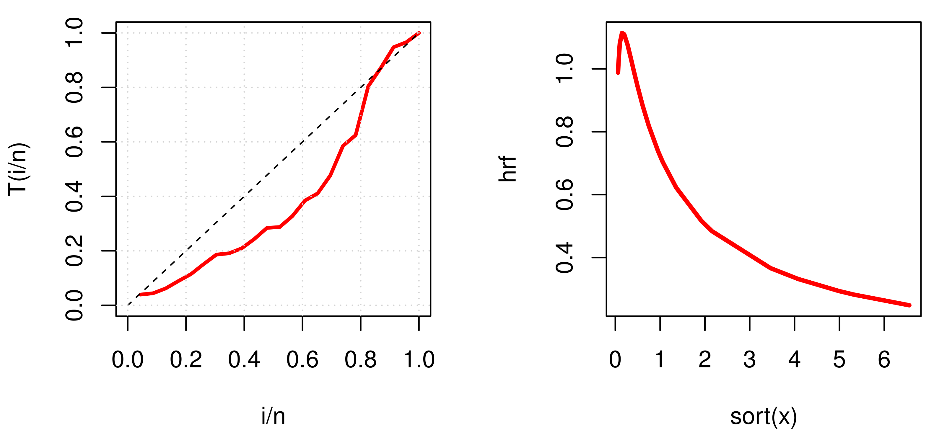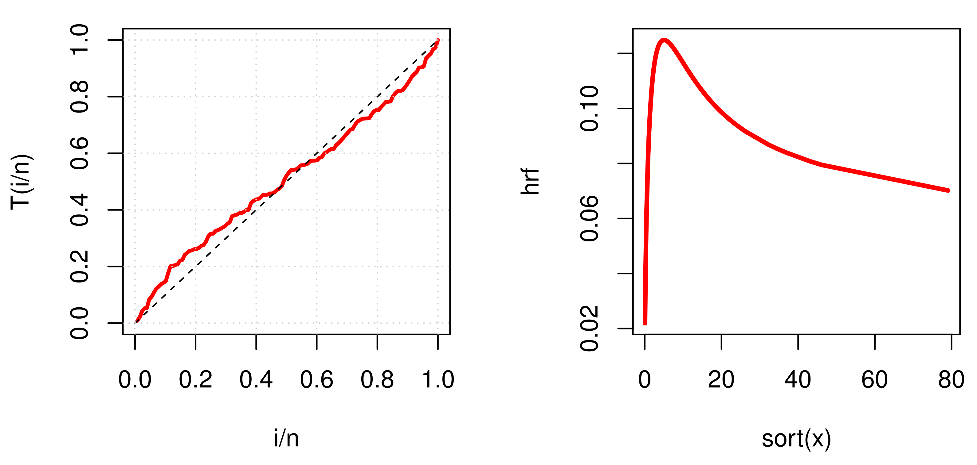Figure 4, Figure 9 and Figure 14 show TTT plots and the estimated hazard for the three real data sets.

6. SSALT Based on PTIC

In this section, the bivariate SSALT under PTIC is described. In addition, the MLE of model parameters is discussed.

6.1. Model Assumptions

The bivariate SSALT under PTIC is as follows: when employing the bivariate SSALT, each stress variable (SV) has two levels. Let $H_s$ be the stress level (SL) s of variable l, where $l=1,2$ and $s=0,1,2$. Normal operational situations are represented by the SLs $H_{10}$ and $H_{20}$. Allow all n units of the experiment to begin at the 1^st step with SLs $(K_{11},K_{21})$ for a time ${\tau }_1$, during which, $n_1$ failures will be recorded. At time ${\tau }_1$, the 1^st SV is raised from $H_{11}$ to $H_{12}$, $c_1$ units are randomly removed from the surviving $N-n_1$ units and the 1^st SV is raised from $H_{11}$ to $H_{12}$. The 2^nd phase is repeated until the predefined time ${\tau }_2$ is calculated at time ${\tau }_2$ from the remaining $N-n_1-c_1-n_2$ units. At the end of the 2^nd step, the other SV is raised from $H_{21}$ to $H_{22}$. The test is repeated until T is attained, at which time, $n_2$ units fail this stage. At time T, all of the remaining surviving units $c_3=N-n_1-c_1-n_2-c_2-n_3$ are removed from the test. For more of an explanation, see Figure 2.

In the 1^st phase, the life of test units is determined by a KMEW distribution with cdf in Equation (6).

The scale parameter ${\alpha }_i$ at test step i has a log-linear function of SLs for $i=1,2,3$.

Step 1:

$ln\left({\alpha }_1\right)=B_0+B_1{H}_{11}+B_2{H}_{21}$.

Step 2:

$ln\left({\alpha }_2\right)=B_0+B_1{H}_{12}+B_2{H}_{21}$.

Step 3:

$ln\left({\alpha }_3\right)=B_0+B_1{H}_{12}+B_2{H}_{22}$.

where $B_0$, $B_1$ and $B_2$ are unknown parameters that differ depending on the product and the test method. It is considered that the two stresses have no relationship.

The cumulative exposure model is also taken into account. The remaining life in this model is solely determined by the present cumulative failure probability and the current SL, regardless of how the probability is calculated ([40]).

For all SLs, the shape parameter $\beta$ remains constant.

The cdf of the lifetimes of test units for the bivariate SSALT and cumulative exposure models is then

$$F_i\left(x\right)=\frac{e}{e-1}\left\{\begin{array}{cc}\left(1-e^{-{\left[1-e^{-{\left({\alpha }_{1}x\right)}^{\beta }}\right]}^{\theta }}\right)& 0\le x\le {\tau }_1\\ \left(1-e^{-{\left[1-e^{-{\left[{\alpha }_1{\tau }_1+{\alpha }_2(x-{\tau }_1)\right]}^{\beta }}\right]}^{\theta }}\right)& {\tau }_1\le x\le {\tau }_2\\ \left(1-e^{-{\left[1-e^{-{\left[{\alpha }_1{\tau }_1+{\alpha }_2({\tau }_2-{\tau }_1)+{\alpha }_3(x-{\tau }_2)\right]}^{\beta }}\right]}^{\theta }}\right)& {\tau }_2\le x\le T\end{array}\right.,$$

(24)

where $i=1,2,3$. The pdf of bivariate SSALT for this can be written as

$$f_1\left(x\right)=\frac{e\beta \theta {\alpha }_1^{\beta }}{e-1}{x}^{\beta -1}{e}^{-{\left({\alpha }_{1}x\right)}^{\beta }}{\left[1-e^{-{\left({\alpha }_{1}x\right)}^{\beta }}\right]}^{\theta -1}{e}^{-{\left[1-e^{-{\left({\alpha }_{1}x\right)}^{\beta }}\right]}^{\theta }},0\le x\le {\tau }_1,$$

(25)

$$\begin{array}{cc}\hfill f_2\left(x\right)=& \frac{e\beta \theta {\alpha }_2}{e-1}{\left({\alpha }_1{\tau }_1+{\alpha }_2(x-{\tau }_1)\right)}^{\beta -1}{e}^{-{\left({\alpha }_1{\tau }_1+{\alpha }_2(x-{\tau }_1)\right)}^{\beta }}{\left[1-e^{-{\left({\alpha }_1{\tau }_1+{\alpha }_2(x-{\tau }_1)\right)}^{\beta }}\right]}^{\theta -1}\hfill \\ & e^{-{\left[1-e^{-{\left({\alpha }_1{\tau }_1+{\alpha }_2(x-{\tau }_1)\right)}^{\beta }}\right]}^{\theta }},{\tau }_1\le x\le {\tau }_2,\hfill \end{array}$$

(26)

and

$$\begin{array}{cc}\hfill f_3\left(x\right)=& \frac{e\beta \theta {\alpha }_3}{e-1}{\left({\alpha }_1{\tau }_1+{\alpha }_2({\tau }_2-{\tau }_1)+{\alpha }_3(x-{\tau }_2)\right)}^{\beta -1}{e}^{-{\left({\alpha }_1{\tau }_1+{\alpha }_2({\tau }_2-{\tau }_1)+{\alpha }_3(x-{\tau }_2)\right)}^{\beta }}\hfill \\ & {\left[1-e^{-{\left({\alpha }_1{\tau }_1+{\alpha }_2({\tau }_2-{\tau }_1)+{\alpha }_3(x-{\tau }_2)\right)}^{\beta }}\right]}^{\theta -1}{e}^{-{\left[1-e^{-{\left({\alpha }_1{\tau }_1+{\alpha }_2({\tau }_2-{\tau }_1)+{\alpha }_3(x-{\tau }_2)\right)}^{\beta }}\right]}^{\theta }}{\tau }_2\le x\le T.\hfill \end{array}$$

(27)

6.2. Likelihood Function of Bivariate SSALT model

In a bivariate SSALT, assume that $x_{ij},i=1,2,3,j=1,2,\dots ,n_i$ denote the observations derived from a PTIC sample with random deletions. The number of items eliminated from the test at any one moment is distributed binomially, and each unit is excluded with the same probability p. In other words,

$$C_i=\left\{\begin{array}{c}{c}_1\approx binomial(N-n_1,p),\\ c_2|c_1=c_2\approx binomial(N-n_1-n_2-c_1,p),\\ c_3=N-n_1-n_2-n_3-c_1-c_2\end{array}\right.$$

(28)

If $C_i$ is independent of $x_{ij}$ for all i, then the joint log-LLF of the bivariate SSALT model under the PTIC sample is as follows:

$$L(\Theta ,p|C)=L_1\left(\Theta \right)P(c_1,p)P\left(c_2\right|c_1,p),$$

(29)

where

$$L_1(\Theta )=\prod _{i=1}^3\prod _{j=1}^{n_i}{f}_i\left(x_{ij}\right){\left[1-F_i\left(x_{ij}\right)\right]}^{c_i},$$

(30)

where $F_i\left(x_{ij}\right)$ and $f_i\left(x_{ij}\right)$ will be substituted for $F_i\left(x_{ij}\right)$ and $f_i\left(x_{ij}\right)$ in (24)–(27). Finally, the log-LLF is constructed by inserting $L_1(\theta )$. Maximizing the logarithm of the likelihood function instead of the likelihood function itself is frequently easier. The log-LLFs of KMEW based on the bivariate SSALT model under the PTIC sample is

$$\begin{array}{cc}\hfill L_1(\Theta )\propto & \prod _{i=1}^3{\left[\frac{e\beta {\theta }^{\beta }}{e-1}\right]}^n{\alpha }_1^{n_1}\prod _{j=1}^{n_1}{x}_j^{\beta -1}{e}^{-{\left({\alpha }_{1}x\right)}^{\beta }}{\left[1-e^{-{\left({\alpha }_1{x}_j\right)}^{\beta }}\right]}^{\theta -1}{e}^{-(c_1+1){\left[1-e^{-{\left({\alpha }_1{x}_j\right)}^{\beta }}\right]}^{\theta }}\hfill \\ & \times {\alpha }_2^{n_2}\prod _{j=1}^{n_2}{\left({\alpha }_1{\tau }_1+{\alpha }_2(x_j-{\tau }_1)\right)}^{\beta -1}{e}^{-{\left({\alpha }_1{\tau }_1+{\alpha }_2(x_j-{\tau }_1)\right)}^{\beta }}{\left[1-e^{-{\left({\alpha }_1{\tau }_1+{\alpha }_2(x_j-{\tau }_1)\right)}^{\beta }}\right]}^{\theta -1}\hfill \\ & \times e^{-(c_2+1){\sum }_{j=1}^{n_2}{\left[1-e^{-{\left({\alpha }_1{\tau }_1+{\alpha }_2(x_j-{\tau }_1)\right)}^{\beta }}\right]}^{\theta }}{e}^{-(c_3+1){\sum }_{j=1}^{n_3}{\left[1-e^{-{\left({\alpha }_1{\tau }_1+{\alpha }_2({\tau }_2-{\tau }_1)+{\alpha }_3(x-{\tau }_2)\right)}^{\beta }}\right]}^{\theta }}\hfill \\ & \times {\alpha }_3^{n_3}{\left({\alpha }_1{\tau }_1+{\alpha }_2({\tau }_2-{\tau }_1)+{\alpha }_3(x_j-{\tau }_2)\right)}^{\beta -1}{e}^{-{\left({\alpha }_1{\tau }_1+{\alpha }_2({\tau }_2-{\tau }_1)+{\alpha }_3(x_j-{\tau }_2)\right)}^{\beta }}\hfill \\ & \times {\left[1-e^{-{\left({\alpha }_1{\tau }_1+{\alpha }_2({\tau }_2-{\tau }_1)+{\alpha }_3(x_j-{\tau }_2)\right)}^{\beta }}\right]}^{\theta -1}.\hfill \end{array}$$

(31)

Table 4. Lifetimes data under bivariate SSALT based on PTIC sample when ${\tau }_1=8,{\tau }_2=13,T=20$.

p	Data	${\mathit{n}}_{\mathit{i}}$	${\mathit{c}}_{\mathit{i}}$
0.1	0.8 0.8 1.3 1.5 1.8 1.9 1.9 2.1 2.6 2.7 2.9 3.1 3.2 3.3 3.5 3.6 4.0 4.1 4.2 4.2 4.3 4.3 4.4 4.4 4.6 4.7 4.7 4.8 4.9 4.9 5.0 5.3 5.5 5.7 5.7 6.1 6.2 6.2 6.2 6.3 6.7 6.9 7.1 7.1 7.1 7.1 7.4 7.6 7.7	49	4
	8.0 8.2 8.6 8.6 8.8 8.8 8.9 8.9 9.5 9.6 9.7 9.8 11.0 11.0 11.1 11.2 11.2 11.5 11.9 12.4 12.5 12.9	22	2
	13.0 13.1 13.3 13.6 13.7 13.9 14.1 15.4 15.4 17.3 18.1 18.2 18.4 18.9 19.0	15	8
0.3	0.8 0.8 1.3 1.5 1.8 1.9 1.9 2.1 2.6 2.7 2.9 3.1 3.2 3.3 3.5 3.6 4.0 4.1 4.2 4.2 4.3 4.3 4.4 4.4 4.6 4.7 4.7 4.8 4.9 4.9 5.0 5.3 5.5 5.7 5.7 6.1 6.2 6.2 6.2 6.3 6.7 6.9 7.1 7.1 7.1 7.1 7.4 7.6 7.7	49	13
	8.0 8.2 8.6 8.8 8.8 8.9 8.9 9.5 9.6 9.7 9.8 11.0 11.0 11.1 11.2 11.2 11.5 11.9 12.4 12.5	20	6
	13.6 13.7 14.1 15.4 15.4 18.9 19.0	7	5
0.5	0.8 0.8 1.3 1.5 1.8 1.9 1.9 2.1 2.6 2.7 2.9 3.1 3.2 3.3 3.5 3.6 4.0 4.1 4.2 4.2 4.3 4.3 4.4 4.4 4.6 4.7 4.7 4.8 4.9 4.9 5.0 5.3 5.5 5.7 5.7 6.1 6.2 6.2 6.2 6.3 6.7 6.9 7.1 7.1 7.1 7.1 7.4 7.6 7.7	49	23
	8.0 8.2 8.6 8.8 9.6 9.7 9.8 11.0 11.0 11.1 11.2 11.5 11.9 12.4 12.5	15	8
	15.4 15.4 18.4	3	2

shows the SLs for lieftime data after bivariate SSALT and PTIC. When ${\tau }_1=8$, ${\tau }_2=13,T=20$,

Table 5. MLE under bivariate SSALT based on PTIC sample for waiting times.

p		$\mathit{\beta }$	$\mathit{\theta }$	${\mathit{\alpha }}_1$	${\mathit{\alpha }}_2$	${\mathit{\alpha }}_3$	AINC	BINC
0.1	estimates	0.5573	6.2110	0.3983	0.4664	0.6876	561.6743	572.0950
	SE	0.5151	5.6768	0.3065	0.3952	0.6279
	CV	0.9242	0.9140	0.7697	0.8473	0.9133
0.3	estimates	0.6484	4.6481	0.2701	0.3574	0.3505	499.5381	509.9587
	SE	0.5921	3.9749	0.2573	0.3288	0.3173
	CV	0.9131	0.8552	0.9527	0.9198	0.9054
0.5	estimates	0.9180	2.5745	0.1450	0.1669	0.1401	446.9478	457.3685
	SE	0.8818	2.9420	0.1392	0.1528	0.1281
	CV	0.9605	1.1427	0.9601	0.9153	0.9141

shows the ML estimators of the model. We may deduce from the data in Table 5 that the model’s efficiency improves when the chance of binomial elimination increases and the AINC and BINC values decrease.

Table 6. Time between failures of secondary reactor pumps data under bivariate SSALT based on PTIC sample when ${\tau }_1=0.6,{\tau }_2=1,T=4.5$.

p	Data	${\mathit{n}}_{\mathit{i}}$	${\mathit{c}}_{\mathit{i}}$
0.1	0.062 0.070 0.101 0.150 0.199 0.273 0.347 0.358 0.402 0.491	10	1
	0.605 0.614 0.954	3	2
	1.060 2.160 3.465 4.082	4	3
0.3	0.062 0.070 0.101 0.150 0.199 0.273 0.347 0.358 0.402 0.491	10	3
	0.605 0.614 0.954	3	2
	1.060 1.359 2.160 3.465	4	1
0.5	0.062 0.070 0.101 0.150 0.199 0.273 0.347 0.358 0.402 0.491	10	5
	0.605 0.954	2	3
	1.06 2.16	2	1

shows the SLs for the time between failures of secondary reactor pumps data after bivariate SSALT and PTIC. When ${\tau }_1=0.6,{\tau }_2=1,T=4.5$,

Table 7. MLE under bivariate SSALT based on PTIC sample for time between failures of secondary.

p		$\mathit{\beta }$	$\mathit{\theta }$	${\mathit{\alpha }}_1$	${\mathit{\alpha }}_2$	${\mathit{\alpha }}_3$	AINC	BINC
0.1	estimates	0.1389	111.8840	107,027.2112	121,853.6131	54,095.2495	54.3313	58.8733
	SE	0.0111	55.5312	5693.4319	5338.5803	6365.0290
	CV	0.0798	0.4963	0.0532	0.0438	0.1177
0.3	estimates	0.1253	150.1647	556,405.5271	987,629.8394	1,211,483.5591	45.2165	49.7585
	SE	0.0098	80.3702	6574.7217	7855.1114	16,817.1504
	CV	0.0780	0.5352	0.0118	0.0080	0.0139
0.5	estimates	0.1202	183.6365	1,327,320.436	1,664,626.840	2,085,033.0914	38.4230	42.9650
	SE	0.0102	112.4214	5187.9587	7103.4757	15,595.2157
	CV	0.0847	0.6122	0.0039	0.0043	0.0075

shows the ML estimates of the model. We may deduce from the results in Table 7 that the model’s efficiency improves when the chance of binomial elimination increases and the AINC and BINC values decrease.

The SLs for bladder cancer data under bivariate SSALT and PTIC are shown in

Table 8. Bladder cancer patients data under bivariate SSALT based on PTIC sample when ${\tau }_1=6$, ${\tau }_2=10,T=20$.

p	Data	${\mathit{n}}_{\mathit{i}}$	${\mathit{c}}_{\mathit{i}}$
0.1	0.08 0.20 0.40 0.50 0.51 0.81 0.90 1.05 1.19 1.26 1.35 1.40 1.46 1.76 2.02 2.02 2.07 2.09 2.23 2.26 2.46 2.54 2.62 2.64 2.69 2.69 2.75 2.83 2.87 3.02 3.25 3.36 3.36 3.48 3.52 3.57 3.64 3.70 3.82 3.88 4.18 4.23 4.26 4.33 4.34 4.40 4.50 4.51 4.87 4.98 5.06 5.09 5.17 5.32 5.32 5.34 5.41 5.41 5.49 5.62 5.71 5.85	62	5
	6.25 6.54 6.93 6.94 6.97 7.09 7.26 7.28 7.32 7.39 7.59 7.62 7.66 7.87 7.93 8.26 8.37 8.53 8.65 8.66 9.02 9.22 9.47 9.74	24	6
	10.06 10.34 10.66 10.75 11.25 11.64 11.79 11.98 12.02 12.03 12.07 12.63 13.11 13.31 14.24 14.76 14.77 14.83 15.96 16.62 17.12 18.10 19.13	23	8
0.3	0.08 0.20 0.40 0.50 0.51 0.81 0.90 1.05 1.19 1.26 1.35 1.40 1.46 1.76 2.02 2.02 2.07 2.09 2.23 2.26 2.46 2.54 2.62 2.64 2.69 2.69 2.75 2.83 2.87 3.02 3.25 3.36 3.36 3.48 3.52 3.57 3.64 3.70 3.82 3.88 4.18 4.23 4.26 4.33 4.34 4.40 4.50 4.51 4.87 4.98 5.06 5.09 5.17 5.32 5.32 5.34 5.41 5.41 5.49 5.62 5.71 5.85	62	18
	6.25 6.54 6.93 6.97 7.09 7.26 7.28 7.32 7.39 7.59 7.62 7.66 7.87 7.93 8.26 8.37 8.53 8.65 8.66 9.02 9.22	21	9
	10.66 10.75 11.79 11.98 13.29 13.31 14.76 14.83 15.96 16.62 17.12	11	7
0.5	0.08 0.20 0.40 0.50 0.51 0.81 0.90 1.05 1.19 1.26 1.35 1.40 1.46 1.76 2.02 2.02 2.07 2.09 2.23 2.26 2.46 2.54 2.62 2.64 2.69 2.69 2.75 2.83 2.87 3.02 3.25 3.36 3.36 3.48 3.52 3.57 3.64 3.70 3.82 3.88 4.18 4.23 4.26 4.33 4.34 4.40 4.50 4.51 4.87 4.98 5.06 5.09 5.17 5.32 5.32 5.34 5.41 5.41 5.49 5.62 5.71 5.85	62	33
	6.25 6.54 6.93 6.97 7.32 7.39 7.62 7.87 8.26 8.53 8.65 8.66 9.02 9.22	14	9
	10.75 11.25 11.79 11.98 13.11 13.31	6	4

. The ML estimators of the model when ${\tau }_1=6,{\tau }_2=10,T=20$ are shown in

Table 9. MLE under bivariate SSALT based on PTIC sample for bladder cancer patients.

p		$\mathit{\beta }$	$\mathit{\theta }$	${\mathit{\alpha }}_1$	${\mathit{\alpha }}_2$	${\mathit{\alpha }}_3$	AINC	BINC
0.1	estimates	1.4459	0.9555	0.0920	0.0773	0.0805	689.4906	700.8987
	SE	1.0425	0.8231	0.0347	0.0456	0.0684
	CV	0.7210	0.8615	0.3775	0.5898	0.8496
0.3	estimates	1.7960	0.7450	0.0848	0.0772	0.0447	602.2144	613.6225
	SE	1.5946	0.7051	0.0265	0.0438	0.0381
	CV	0.8878	0.9464	0.3122	0.5673	0.8527
0.5	estimates	1.4435	0.9564	0.0921	0.0856	0.0634	527.9641	539.3722
	SE	1.2259	0.8965	0.0397	0.0609	0.0609
	CV	0.8492	0.9374	0.4308	0.7119	0.9602

. From the results in Table 9, we conclude that the efficiency of the model increases when the probability of binomial removal increases, where the AINC and BINC values are smaller. In addition, we conclude that the model with p = 0.5 is better than another model. The bladder cancer data set performs quite well, as the five roots of the parameters are global maximums, as seen in Figure 19.

7. Concluding Remarks

In this study, we explored a new three-parameter model that is called the Kavya–Manoharan exponentiated Weibull model. Its statistical and mathematical features (moments, incomplete moments, mean deviations, Bonferroni and Lorenz curves, entropy and order statistics) were derived. The maximum likelihood estimation of the parameters was discussed. The relevance and flexibility of the KMEW model were demonstrated using two real datasets. A bivariate SSALT based on PTIC for the KMEW model was introduced. Minimizing the asymptotic variance of the MLE of the log of the scale parameter at design stress under PTIC data yields an expression of an ideal test plan under PTIC. In Table 6 and Table 8, we compared the different schemes based on different values of binomial removals. From these results, we note that, if the value of binomial removals increases, then the efficiency of this model increases. For future directions, the new suggested model is very interesting to study. Many authors can estimate the parameters of the suggested model under different censored schemes. This work requires a remarkable increase in investigation, which we will delegate to future research.