Fledgling Quantum Spin Hall Effect in Pseudo Gap Phase of Bi2212

Abstract

We studied the emergence of the quantum spin Hall (QSH) states for the pseudo-gap (PG) phase of Bi2212 bilayer system, assumed to be D-density wave (DDW) ordered, starting with a strong Rashba spin-orbit coupling (SOC) armed, and the time reversal symmetry (TRS) complaint Bloch Hamiltonian. The presence of strong SOC gives rise to non-trivial, spin-momentum locked spin texture tunable by electric field. The emergence of quantum anomalous Hall effect with TRS broken Chiral DDW Hamiltonian of Das Sarma et al. is found to be possible.

1. Introduction

The onset of the pseudo-gap (PG) in cuprates is defined by the opening of an anti-nodal gap and the reduction of the large Fermi surface to Fermi arc [1,2,3,4,5,6,7,8,9,10,11,12], as in the Wyle/Dirac semimetal. The exact nature of PG still remains an enigma [7,8,9,10,11,12,13,14,15,16,17,18,19,20,21,22]. According to some investigators [1,2,3,4,5,6,7,8,9,10,11], it corresponds to a distinct phase akin to an unconventional metal or a symmetry preserved/broken state. On the other hand, the competing hidden order ideas, such as the $d_{x^2-y^2}$-density wave (DDW), order in refs. [1,2,3,4] associated with the pairing in particle–hole channel, portray pseudogap (PG) as a hidden order parameter not detectable by usual s-wave probes by producing charge current, magnetic moment, etc. Apart from this, some of the other formulations are given below: (i) The advocacy of phase fluctuations and/or precursor but incoherent pairing correlations [11,12] for the PG phase. (ii) The BCS-BEC crossover scenario [13,14] where there is no hidden symmetry breaking or competing order. The same microscopic origin and the same symmetry are shared by the complex superconducting gap and the real pseudo-gap. The latter is real, due to the phase decoherence. (iii) The pseudo-gap arising from some instability, such as spin or orbital current, charge ordering, not related to pairing [5,6,15]. (iv) The origin of PG from a pair-density wave (PDW) [16,17], which is an unusual form of electron organization involving electron pairing on the same side of the Fermi surface. It may be mentioned that a PDW in Bi2212 was observed using a superconducting STM tip [18] in the absence of magnetic field. (v) The entanglement of two kinds of preformed pairs in the particle–particle and particle–hole channels [19], giving rise to the formation of PG. This theoretical formulation regards PG formation as the one which corresponds to a phase transition, and not a crossover.

In this paper we begin with a Bloch Hamiltonians with strong Rashba spin-orbit coupling (RSOC) for the pseudo-gap (PG) phase of Bi₂Sr₂CaCu₂O_8+δ (Bi2212) bilayer system. Apart from RSOC, the Hamiltonian involves DDW order [1,2,3,4] and therefore possesses time-reversal symmetry (TRS). The Hamiltonian also involves a term accounting for the effect of coupling between different CuO₂ planes. The microscopic origin of RSOC lies in the non-equivalence of two layers in the bilayer system. Whereas one Cu-O layer has Ca ions above and Bi-O ions below, in the unit cell of the other layer, this situation is reversed. This leads to a nonzero electric field E within the unit cell. We find spin-momentum locking (SML) in momentum space, which suggests the presence of a strong spin-orbit coupling in Bi2212 like a topological insulator. A recent spin- and angle-resolved photoemission spectroscopy measurement for Bi₂Sr₂CaCu₂O_8+δ had reported [6] a non-trivial spin texture, which corresponds to a well-defined direction for each electron real spin depending on its momentum. Since the origin of PG has been under heated debate [7,8,9,10,11,12,13,14,15,16,17,18,19,20,21,22] for the past three decades, a relevant question is why identify PG phase of cuprates with the DDW order when bewildering varieties of formulations [7,8,9,10,11,12,13,14,15,16,17,18,19,20,21,22,23] are present. The paramount reason is that the entropy difference between the PG phase with DDW order and normal paramagnetic states was found to be negative [4], leading to the establishment of PG formation as the onset of the first order phase transition. However, the outcome of the torque magnetometry experiment [20] has recently figured out what is going on in PG phase on the transition/crossover issue. This experiment has provided the thermodynamic evidence that the pseudo-gap onset in cuprates, such as YBCO (barium copper yttrium oxide), BSCCO (Bismuth strontium calcium copper oxide), and LSCO (Lanthanum strontium copper oxide), which have a layered structure with charge carriers moving in the copper-oxide planes, are associated with a second-order nematic phase transition. Nonetheless, we have opted to associate PG state with DDW order apart from parity because, as well as translational and rotational symmetry breaking, it exhibits some topological features [21]. Moreover, if the DDW order is responsible for the PG phase, then the gap does not get affected by magnetic field in the underdoped regime; the dependence springs up [22] as soon as the gap vanishes in the over-doped regime. This is consistent with the experimental data [23].

We investigate the possibility of occurrence of the quantum spin Hall (QSH) effect in Bi2212 in this paper. In general, having two quantum Hall insulating layers one over the other leads to a trivial insulator. However, our band structure-based detailed analysis in Section 2 has indicated that Bi2212 bilayer geometry will have access to QSH [24] phase. The latter is ensured in a DDW order-based description of the semi-metallic PG state, provided we have the invariance of TRS and strong spin-orbit (SO) coupling. In contrast, Zhao et al. [24] recently have proposed two different experiment to show that QSH upshot is possible through relativistically generated quantum spin Hall Hamiltonian in 2D metals of Corbino geometry surrounding a solenoid in the absence of SOC. The stark difference between this finding and that of ours highlights the fact that the Fermi surface structure and the geometry are the two aspects which decide the requirements to access QSH phase. On a quick side note, since an individual Corbino disk could be regarded as a qubit, it was surmised by Zhao et al. [24] that a hexagonally packed array of thermally-managed solenoids, each carrying stacks of thermally-managed 2D metallic Corbino disks surrounding it, could then facilitate fault-tolerant quantum computation. In our case, in principle, the osillatory magnetic field induced by the SO coupling can manipulate electron spin. Furthermore, by means of gigahertz, electric field coherent manipulation of individual electron spin is ideally possible by electron dipole spin resonance (EDSR) technique, as in the case of a GaAs/AlGaAs gate defined quantum dots [25]. The EDSR allows the orientation of the spin magnetic moment to flip using electro-magnetic radiations at resonant frequencies. This leads to formation of SO qubits which, in turn, leads to clearing the way for a computing architecture [26] that can scale up to meet increased workloads. Although a topical issue, it is beyond the scope of the paper.

When TRS is broken in a 2D system, say, due to the presence of the magnetic impurities (but no magnetic field), the system spontaneously crosses over to quantum anomalous Hall (QAH) phase at low temperatures [27]. The $d_{xy}+i d_{x^2-y^2}$ (Chiral DDW) ordered phase [5] also leads to broken TRS. Our contention is that, with or without proximity to magnetic impurities, this state will display QAH effect. In Section 3 we discuss the quantum anomalous Hall (QAH) effect, replacing the DDW order with CDDW order and incorporating the strong RSOC. The imaginary part of the CDDW order parameter D_k = (−χ_k + i$∆$_k) breaks TRS. The functions (χ_k, $∆$_k) are given by [5] χ_k = −(χ₀/2) sin(k_xa) sin(k_ya), $∆$_k = ($∆$₀^(PG) (T)/2)(cos k_xa − cos k_ya), and k = $\left( k_x, k_y \right).$ The ordering wave vector Q is taken to be Q = (Q₁ = ±π, Q₂ = ±π). It is important to mention that the onset of CDDW ordering leads to a peak in the anomalous Nernst signal (ANS) [5]. The main contribution to this chirality induced ANS comes from the points (±π(1 − φ), ±πφ),(±πφ, ±π(1 − φ)) with φ~0.2258 located roughly on the boundary of the Fermi pockets in the momentum space (cf. ref. [5]). We take due care of this observation in Section 3. A prominent indicator of QAH effect is the quantum transition in the transverse Hall resistance accompanied by a considerable drop in longitudinal resistance. For a perfect crystal, this effect is intrinsically quantum-mechanical as it involves the Berry-curvature, which calls for Bloch state eigen wavefunction.

The paper is organized as follows. In Section 2 we derive an expression for the single-particle excitation spectrum in PG state and discuss QSH effect. Additionally, random disorder potential and mass term will be introduced to determine their effect on anti-nodal/nodal gap. In Section 3, we carry out an investigation of the QAH effect. The paper ends with a brief discussion and conclusions in Section 4.

2. Quantum Spin Hall Insulator

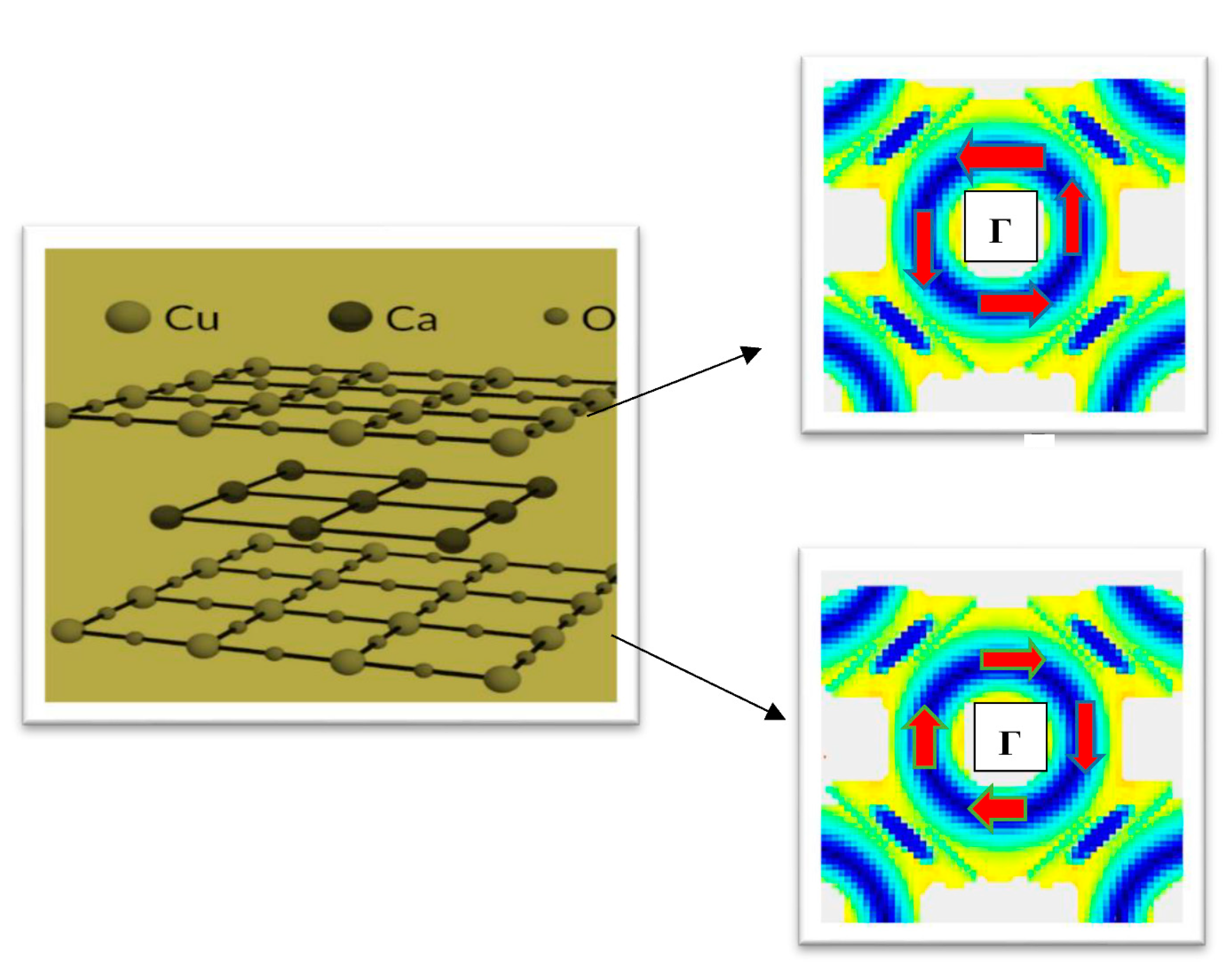
The cuprate Bi2212 consists of CuO₂ layers separated by spacer layers as in Bi2212, as shown in Figure 1. The total dispersion for non-interacting system, together with the effect of coupling between different CuO₂ planes, can be written as $ϵ\left(k,k_z\right)$= ${\epsilon }_{k }$+ ${\epsilon }_{\begin{array}{c}{k}_z\\ \end{array}}\left(k\right),$ where ${\epsilon }_{k }=e_{k }-\mu ,$k and k_z, respectively, denote the in-plane and out-of-plane components of K = (k, k_z). The term $\mu$ stands for the chemical potential of the fermion number. The dispersion $e_{k }=-2t P_1\left(k\right)+4t^{\prime }{P}_2\left(k\right)-2t^{″}{\mathrm{P}}_3\left(k\right)-4t^{‴}{P}_4\left(k\right)$ including the in-plane first (nearest neighbor abbreviated as NN below), the second, the third neighbor, and the fourth neighbor hoppings. Here, $P_1\left(k\right)=\left(s_x\left(a\right)+s_y\left(a\right)\right), P_2\left(k\right)=s_x\left(a\right)$) $s_y\left(a\right),$ $P_3\left(k\right)=\left({ s}_x\left(2a\right)+{ s}_y\left(2a\right)\right), {\mathrm{and} P}_4\left(k\right)=\left(s_x\left(a\right)s_y\left(2a\right)+s_x\left(2a\right)s_y\left(a\right)\right)$. For the hole-doped (electron-doped) materials, t₁ > 0 (t₁ < 0), and, in all cases, t₁ < (t/2). The ${\epsilon }_{\begin{array}{c}{k}_z\\ \end{array}}$(k) term accounts for the effect of coupling between different CuO₂ planes, and possesses the following form for bilayer Bi2212 [28,29]: ${\epsilon }_{\begin{array}{c}{k}_z\end{array}}\left(\mathit{k}\right)$ = −ϒ_z(k, s_z(c/2))[(s_x(a) − s_y(a))²/4 + a₀], where c denotes the lattice constant along the z-axis, and the term

$${{\mathsf{\Upsilon }}_{\mathrm{z}} (k, s_z(c/2\left)\right)=\pm [{t_p}^2+16 t_{in}^2{s}_x^2\left(\frac{a}{2}\right)s_{\mathrm{y}}^2\left(\frac{a}{2}\right)+8t_p{t}_{in}{s}_x\left(\frac{a}{2}\right)s_y\left(\frac{a}{2}\right)s_z\left(\frac{c}{2}\right)]}^{1/2}.$$

Here, $t_p$ is an effective parameter for hopping within a single bilayer, i.e., it controls the intracell bilayer splitting and s_j(a) ≡ cos(k_ja) [28,29]. The compound Bi2212, however, also involves intercell hopping ($t_{in}$). The intra-layer coupling $t_p$ and the intercell coupling $t_{in}$ are both quite substantial, as are the in-plane hopping terms beyond the NN term. The plus (minus) sign refers to the bonding (anti-bonding) solution. The term c_z arises because, supposedly, we have an infinite number of stacked layers. Along the high symmetry line X(π,0) – M(π,π), we have ϒ_z = ±t_p. This leads to a lack of k_z-dispersion along this high-symmetry line, for ${\epsilon }_{\begin{array}{c}{k}_z\end{array}}\left(\mathit{k}\right)$ →${\epsilon }_{\begin{array}{c}{k}_z\end{array}}\left(k_y\right)$ = ±(1/4) $t_p$ [(1 + $s_y{\left(a)\right)}^2+4a_0$]. The additional hopping $a_0$ allows for the presence of a splitting at Γ(0,0). It is reported [30] that adequate control of the interlayer spacing, albeit the interlayer hopping in Bi-based superconductors, is possible through the intercalation of guest molecules between the layers. This could be a way to tune the hopping parameter. All energies in our calculation below are expressed in units of the first neighbor hopping as this corresponds to the kinetic energy and therefore the most dominant; the second-neighbor hopping in the dispersion, which is known to be important for cuprates [1,2,3,4,5,6], frustrates the kinetic energy of electrons. Therefore, in what follows, we render the first to the fourth neighbor hoppings, the couplings $t_p$ and $t_{in}$, the quantities (χ₀,$∆$₀^(PG)), and the terms to be introduced below, viz. the intra-layer Rashba spin-orbit coupling, the disorder potential, and the mass term, dimensionless dividing by the first neighbor hopping term. The exchange energy parameter in Section 3, which will be denoted by the symbol M, will also be in the first neighbor hopping energy units.

Our decision to associate DDW order of Chakravorty et al. [1,2,3,4] with PG state demands that we need to consider the interaction U_x2−y2(k,k′) = U₁ (cosk_xa − cosk_ya)(cosk′_xa − cosk′_ya) for the formation of the pairing in the particle–hole channel. If we further assume that the order parameter in superconducting state has d-wave symmetry, we may sound like advocates of pre-formed Cooper pair formation [31,32]. This is not true, as has been explained in the second paragraph in Section 1. Additionally, motivated by the findings of Vishwanath et al. [7], we introduce the intralayer Rashba spin-orbit coupling (RSOC) as a special ingredient. Suppose now tht d_k,σ (σ = $\uparrow \downarrow \mathrm{for} \mathrm{the} \mathrm{real} \mathrm{spin}$) corresponds to the fermion annihilation operator for the single-particle state {k= $\left(k_x, k_y\right)$,σ} in a single layer of the system. In the basis ($d_{\mathrm{k}, \uparrow }^{†}$ $d_{\mathrm{k},\downarrow }^{†} d_{\mathrm{k}+\mathrm{Q}, \uparrow }^{†} d_{\mathrm{k}+\mathrm{Q},\downarrow }^{†})$^T$,$ we consider a $2 D \mathrm{momentum} \mathrm{space}$ single-layer Hamiltonian.

$$H\left(k_x, k_y\right)=\left(\begin{array}{cc}{H}_0\left(k_x, k_y\right)& Ϛ\left(k_x, k_y\right)\\ {Ϛ}^{*}\left(k_x, k_y\right)& H_0\left(k_x+Q_1, k_y+Q_2\right)\end{array}\right)$$

(1)

to describe the pseudo-gap phase of the system involving CDDW order given by the matrix $Ϛ\left(k_x, k_y\right)=\left(\begin{array}{cc}{D}_k^{†}& 0\\ 0& D_k\end{array}\right), \mathrm{where} D_k=\left(-{\chi }_k+\mathrm{i}{∆}_k\right)$ $\mathrm{breaks} \mathrm{the} \mathrm{parity} \mathrm{and} \mathrm{the} \mathrm{time}$ reversal symmetry (TRS) of the normal state. The term ${\epsilon }_{\begin{array}{c}{k}_z\\ \end{array}}\left(k\right)$ will be incorporated later (see Equation (5)). The matrix

$$H_0\left(k,\mu \right)=\left(\begin{array}{cc}{\epsilon }_k& \alpha \left(k_x, k_y\right) \\ {\alpha }^{*}\left(k_x, k_y\right) & {\epsilon }_k\end{array}\right)$$

(2)

where the intra-layer Rashba spin-orbit coupling $\left(\mathrm{RSOC}\right)\alpha \left(k_x, k_y\right)={\alpha }_k={\alpha }_0$(−isin(k_xa) − (k_ya)). That will not be all. Since ${\alpha }_1\left(k_x, k_z\right)$ = ${\alpha }_1\left({\sigma }_{\mathrm{z}}\sin \left(k_x{a}_x\right)-{\sigma }_{\mathrm{x}}\sin \left(k_z{a}_z\right)\right)$—a giant anisotropic 3D Rashba-like inter-layer coupling (here $\mathbf{\sigma }$ are Pauli spin matrices and a is the lattice constant) has been directly observed by spin-ARPES [33], we ideally need to consider the effect of this term for the present quasi two-dimensional system. In ref. [33], investigators observed emergence of large spin splitting at the M points of the Brillouin zone instead of the Γ point, where Rashba type splitting is usually found. We have not considered this interlayer RSOC (${\alpha }_1\left(k_x, k_z\right))$ here, assuming it to be small compared to the other terms in $E_j\left(s,\sigma ,k, k_z\right).$ The quantity ${\alpha }_0$ is the RSO coupling strength, which is proportional to the strength of the nonzero electric field E, mentioned in the first paragraph of Section 1, assumed to be in the z = z $\widehat{\mathit{z} }$ direction. It is informative to see how $\alpha \left(k_x, k_y\right) \mathrm{and} {\alpha }_1\left(k_x, k_z\right) \mathrm{originate}$ from the generalized SO coupling and estimate the electric field (${\mathit{E}}_{{\alpha }_0})$ corresponding to SO coupling $\alpha \left(k_x, k_y\right)$. The generalized SO coupling Hamiltonian is $H_{so}^z={\alpha }_0 (\mathit{\sigma }\times$ ak). $\widehat{\mathit{z} }$ =${\alpha }_0 \mathit{\sigma }·\left(a\mathit{k}\times \widehat{\mathit{z} }\right).$ Introducing the momentum dependent Zeeman-like magnetic field ${\mathit{B}}_{{\alpha }_0}\left(k\right)$ due to RSOC, one may also write $H_{so}^z=\left(\frac{1}{2}\right){\mu }_{B}g(\mathit{\sigma }·{\mathit{B}}_{{\alpha }_0}) \mathrm{where} {\mathit{B}}_{{\alpha }_0}=\left(\frac{2{\alpha }_0}{g{\mu }_B}\right) \left(a\mathit{k}\times \widehat{\mathit{z} }\right).$ The comparison of the two expressions for $H_{so}$ will lead to an expession for the momentum dependent electric field $E_{{\alpha }_0}$ as $E_{{\alpha }_0}\left(k\right)=$ (2cα_0/gμ_B)(ak) in the z-direction. $\mathrm{This} \mathrm{is} \mathrm{the} \mathrm{electric} \mathrm{field} \mathrm{corresponding} \mathrm{to} \mathrm{the} \mathrm{intra}-\mathrm{layer} \mathrm{Rashba} \mathrm{coupling}. \mathrm{Here},$ ${\mu }_B=9.27\times {10}^{-24}$ J/T $\mathrm{is} \mathrm{the}$ Bohr magneton. The substitution of the numerical values leads to a strong electric field of the order 10⁴ V ${\mathrm{nm}}^{-1} \mathrm{at} \mathrm{the} \mathrm{nodal} \mathrm{and}$ $\mathrm{the}$ anti-nodal regions. This can be tuned by gate voltage. Similarly, in view of the generalized SO coupling above, one obtains $H_{so}^x$ $\mathrm{and} H_{so}^y, \mathrm{where} \mathrm{the} \mathrm{latter} \mathrm{is} {\alpha }_1(\mathit{\sigma }\times$ ak). $\widehat{\mathit{y} }$= ${\alpha }_1 \mathit{\sigma }·\left(a\mathit{k}\times \widehat{\mathit{y} }\right)={\alpha }_1\left({\sigma }_z{k}_x{a}_x-{\sigma }_x{k}_z{a}_z\right) .$ As regards the e-e interactions, $U {{\displaystyle \sum }}_i$ $d^{†}{}_{i\uparrow } d_{i\uparrow } d^{†}{}_{i\downarrow } d_{i\downarrow }$ is the onsite repulsion of d electrons, where the intra-layer d electrons are locally interacting via a Hubbard-U repulsion. We have not considered this term, assuming the correlation effect are marginally relevant. As noted above, the Hamiltonian (1) is suitable to investigate the QAH state. For the QSH state, we have D_k = $∆$_k = ($∆$₀^(PG) (T)/2)(cos k_xa–cos k_ya), which breaks the parity only. The investigation is expected to show spin-momentum locking in some regions of BZ. Furthermore, we have not introduced random disorder potential and mass term in the Hamiltonian in (1) here. These terms will be introduced in Section 2 to determine their effect on anti-nodal/nodal gap.

The eigenvalues ${\in }_j\left(s,\sigma ,k\right),$ where j = 1,2,3,4, $\sigma =\pm 1$ is the spin index and $s$ $=\pm 1$ is the band-index, are derivable from the Hamiltonian (1)$, \mathrm{suitable} \mathrm{to} \mathrm{investigate} \mathrm{QAH} \mathrm{effect},$ and are given by the quartic ${\in }_j$⁴ + a_A (k) ${\in }_j$³ + b_A(k) ${\in }_j$² +c_A(k) ${\in }_j$+ d_A(k) = 0. In view of the Ferrari’s solution of a quartic equation, we find the roots as

$${\in }_j\left(s,\sigma ,k\right)= \sigma \sqrt{\frac{{\eta }_0\left(k\right)}{2}}+{\epsilon }_k{}^U+s {\left(b_0\left(k\right)-\left(\frac{{\eta }_0\left(k\right)}{2}\right)+\sigma c_0\left(k\right)\sqrt{\frac{2}{{\eta }_0\left(k\right)}} \right)}^{\frac{1}{2}} .$$

(3)

Since the spin index $\sigma$ appears twice in (3), the term $\sigma$ $\sqrt{\frac{{\eta }_0\left(k\right)}{2}}$ does not act like Zeeman magnetic energy. The coefficients are a_A(k) = $-4{\epsilon }_k{}^U$, ${\epsilon }_k{}^U$= (${\epsilon }_k$ + ${\epsilon }_{k+Q})/2$, b_A(k) = $\{4{\epsilon }_k{}^{U^2}+2({\epsilon }_k {\epsilon }_{k+Q}-$$|D_k {|}^2)-$ $|{\alpha }_k {|}^2-$ $|{\alpha }_{k+Q} {|}^2$}, c_A(k) = $-4{\epsilon }_k{}^U({\epsilon }_k {\epsilon }_{k+Q}-$$|D_k {|}^2)-$2ε_k+Q |${\alpha }_k {|}^2-$2${\epsilon }_k |{\alpha }_{k+Q} {|}^2$, d_A(k) = $({\epsilon }_k {\epsilon }_{k+Q}-$$|D_k {|}^2)$² $-{\epsilon }_{k+Q}^2 \left|{\alpha }_k {|}^2-{ \mathsf{\epsilon }}_{\mathrm{k}}^2 \left|{\alpha }_{k+Q} {|}^2+\right|{\alpha }_k {|}^2 \right|{\alpha }_{k+Q} {|}^2+F\left(k_x, k_y\right)$, where $|D_k {|}^2=\left({\chi }_k^2+{∆}_k^2\right)$, ${\alpha }_k={\alpha }_0$(−isin(k_xa)− sin(k_ya)) and $F\left(k_x, k_y\right)=-2{\alpha }_0^2\left({\chi }_k^2-{∆}_k^2\right) f\left(k_x, k_y\right)-4{\alpha }_0^2\left({\chi }_k{∆}_k\right) g\left(k_x, k_y\right),$ $f\left(k_x, k_y\right)=[$ sin(k_xa)sin(k_xa + Q₁) + sin(k_ya)sin(k_ya + Q₂)], and $g\left(k_x, k_y\right)=[$ sin(k_xa) sin (k_ya + Q₂) $-$ sin(k_ya)sin(k_xa + Q₁)]. The functions appearing in (2) are given by

$${\eta }_0\left(k\right)=\frac{2b_0\left(k\right)}{3}+{\left({∆}_1\left(k\right)-{∆}_0\left(k\right)\right)}^{\frac{1}{3}}-{\left({∆}_1\left(k\right)+{∆}_0\left(k\right)\right)}^{\frac{1}{3}},$$

(4)

$$\begin{gathered} {∆}_0\left(k\right)=(\frac{b_0^3\left(k\right)}{27}-\frac{b_0\left(k\right)d_0\left(k\right)}{3}-c_0^2\left(k\right)), \\ {{∆}_1\left(k\right)=(\frac{2}{729}{b}_0^6+\frac{4d_0^2{b}_0^2}{27}+c_0^4-\frac{d_0{b}_0^4}{81}-\frac{2b_0^3}{27}+\frac{2c_0^2{b}_0{d}_0}{3}+\frac{d_0^3}{27})}^{1/2}, \end{gathered}$$

(5)

$$\begin{gathered} b_0\left(k\right)=\left\{\frac{3a_A^2\left(k\right)-8b_A\left(k\right)}{16} \right\}, c_0\left(k\right)=\left\{ \frac{-a_{A }^3\left(k\right)+4a_A\left(k\right)b_A \left(k\right)-8c_A \left(k\right)}{32} \right\} \\ {d}_0\left(k\right)=\frac{-3a_{A }^4\left(k\right)+256d_A\left(k\right)-64a_A\left(k\right)c_A\left(k\right)+16a_A^2\left(k\right)b_A\left(k\right)}{256}. \end{gathered}$$

(6)

In order to investigate QSH effect, we need to have invariant TRS. Therefore, we have to make the following substitutions: ${\chi }_k=0,$$|D_k {|}^2={∆}_k^2$,$\mathrm{and} F\left(k_x, k_y\right)=2{\alpha }_0^{2 }{∆}_k^2 \left[\sin \left(k_{x}a+Q_1\right)\sin \left(k_{x}a \right)+\sin \left(k_{y}a\right)\sin \left(k_{y}a+Q_2\right)\right].$ For the bilayer system, the energy eigenvalues are given by $E_j\left(s,\sigma ,k, k_z\right)=$ ${\in }_j\left(s,\sigma ,k\right)\pm {\epsilon }_{\begin{array}{c}{k}_z\\ \end{array}}\left(k\right)$ for the bonding as well as the anti-bonding.

The plots of energy bands ${\in }_j\left(s,\sigma ,k\right)$ in (3) in the QSH case belonging to the nodal and anti-nodal regions, as well as at Γpoint, are shown in Figure 2. We have also shown the calculated Fermi surfaces (FS), including the near-neighbor hopping and RSOC, in the absence of DDW order (Figure 2a) and in the presence of it (Figure 2b). Here, the Fermi surfaces are hole-like surfaces. In Figure 2a, the reduced Brillouin zone (BZ) is shown in red, and constant-energy contours are shown in blue. In Figure 2b, we have the calculated FS with electron pockets in red and hole pockets in black. The dispersion now has the periodicity of BZ. The numerical values of the parameters to be used in the calculation/graphical representation are t = 1, t′/t = −0.28 (hole-doping), t″/t = 0.1, t‴/t = 0.06, t_p/t = 0.10, t_in/t = 0.10, $\frac{{\alpha }_0}{t}=0.30, \frac{a_0}{t}=0.20, c{k}_z=2.3, \mathrm{and}$ $∆$₀^(PG) (T)/t = 0.50. The state dispersion is perfectly nested with the ordering wave vector Q = (Q₁ = ±π, Q₂ = ±π). The reason for taking $c{k}_z=2.3$ is that, in the 2D-plot of the z-direction dispersion as a function of the dimensionless wave number $c{k}_z$ at the nodal ($a{k}_{\mathrm{x}}=\frac{\pi }{2},a{k}_{\mathrm{y}}=\frac{\pi }{2}) \mathrm{point}, \mathrm{we} \mathrm{find}$ that the dispersion attains the maximum value at $c{k}_z$ = 2.3 (see Section 4). Throughout the whole paper, we choose 𝒕 to be the unit of energy, as already stated. Effectively, it means all the quantities involved in the system Hamiltonian are made dimensionless, dividing by 𝒕. On a quick sidenote, we envisage a situation in which the chemical potential or Fermi energy E_F of a potential QSH system intersects a band either an even or odd pair number of times in the same BZ. If there is an odd number of pair intersections at time-reversal-invariant-momenta (TRIMs) (which guarantees the time reversal invariance), the system state is topologically non-trivial (strong topological insulator), and disorder or correlations cannot remove pairs of such surface state crossings (SSC) by pushing the surface bands entirely above or below the Fermi energy E_F. This has been checked by assigning different values to the chemical potential (see Figure 2c,d). We notice that the number of paired SSCs in each of the figures in Figure 2 is odd (one). We also notice that $a{\mathrm{k}}_{\mathrm{trim}}=\left(3,\frac{\pi }{2}\right),\left(1,\frac{\pi }{2}\right)$, (2,π), (1,0) in Figure 2c, d, e and f respectively. The vertical lines are the indicators of time reversal invariant momenta (TRIM). Amongst the pair of TRI momentum (K, $-$K), the relation $-\mathit{K}=\mathit{K}+\mathit{G}$ is satisfied. When there are even number of pairs of surface state crossings, the surface states are topologically trivial (weak TI or conventional insulator) for disorder, or correlations can remove pairs of such crossings, insulator, or a strong topological insulator. The material band structures are characterized by Kane–Mele index Z₂ = +1 (${\nu }_0$ = 0) and Z₂ = −1 (${\nu }_0$ = 1). The former corresponds to weak TI, while the latter corresponds to strong TI. In the Appendix A, we calculate the topological invariant ${\nu }_0$ to characterize the present TRS preserving system in a similar manner, as formulated by Fu and Kane [34,35], helped by the graphics in Figure 2. The help is required, as the inclusion of the Rashba coupling leads to non-conservation of spin [34] (see the note above Equation (8)). As ${\nu }_0$ turns out to be 1 (see the Appendix A), we find the system Hilbert space to be twisted [34,35]. The physical consequence of the nontriviality is the appearance of topologically-protected surface states. The Bi2212 layer, therefore, comprises of ‘helical liquids’ [36] in the monolayer (2D) geometry in the long wavelength limit. In this limit, $\sin \left(a_j{k}_j\right) \to a_j{k}_j \mathrm{and} \cos \left(a_j{k}_j\right)\mathrm{and} \cos (a_j{k}_j)\to \left(1-\frac{a_j^2{k}_j^2}{2}\right)$ where j = (x, y, z), and $a_j$ is the lattice constant along j direction. The helicity is one of the most unique properties of a topologically protected surface. These lead to the conclusion that the system considered is a strong TI or a QSH material. A recent report of a spin-signal on the surface by the inverse Edelstein effect [37] has confirmed the helical spin-structure.

A spin version of quantum Hall effect is called QSH effect. As we have stated, a QSH system possesses a twisted Hilbert space, leading to a pair of helical edge states with opposite spins propagating in opposite directions. Such non-trivial states with spin-momentum locking gives rise to two-dimensional topological insulator. In what follows, we provide the outline of a method to determine the effect of non-magnetic, random disorder potential and a mass term on the anti-nodal/nodal gap of the present system. We apply a novel technique published by Katsura and Koma [38,39]. The exercise is also motivated by the works in the refs. [40,41] in the context of metal-insulator transition in semiconductors. In the basis ($d_{\mathrm{k}, \uparrow }^{†} d_{\mathrm{k},\downarrow }^{†}{d}_{\mathrm{k}+\mathrm{Q}, \uparrow }^{†}{d}_{\mathrm{k}+\mathrm{Q},\downarrow }^{†} {)}^{†}$, the starting Hamiltonian in Equation (1), together with the Rashba coupling term in the DDW ordered phase (for the ordering vector Q = (Q₁ = ±π, Q₂ = ±π), may be written in a compact form as

$$H\left(k_x, k_y\right)=({\epsilon }_k+W_0) {\tau }_3\otimes s_0+D_k {\tau }_1\otimes s_0+(∆-g_1) {\tau }_3 \otimes s_1+g_2 {\tau }_3 \otimes s_2$$

(7)

where the additional terms introduced are $W_0$ and $∆.$ The term $W_0$ corresponds to a RDP, which has continuous uniform distribution in the interval [−W/2, W/2] with a positive parameter W. If a uniform distribution is continuous (discrete), it has an infinite (finite) number of equally likely measurable values. The symbol $∆$ stands for the mass term. We shall treat this model below in the long wave-length limit. The matrices τ_j and s_j (j = x, y, x) are Pauli matrices for the orbital and the spin, respectively. Additionally, $g_1={\alpha }_0$ sin(k_ya) and $g_2={\alpha }_0$ sin(k_xa). These terms correspond to RSOC. Upon recalling that spin component ${{\displaystyle \sum }}_j=\left(\begin{array}{cc}{s}_{\mathrm{j}}& 0\\ 0& s_{\mathrm{j}}\end{array}\right),$ we find that the commutator $\left[\left(\mathsf{\Delta }-g_1\right){\tau }_3\otimes s_1+g_2{\tau }_3\otimes s_2, {{\displaystyle \sum }}_z\ne 0\right]$. This means, due to the presence of RSOC, the spin $s_z$ is not conserved. For the CDDW order, the corresponding Hamiltonian with random disorder potential and mass term will appear as

$$\begin{array}{cc}\hfill H\left(k_x, k_y\right)=\left(\frac{1}{2}\right){\epsilon }_k{\tau }_0& \otimes \left({ s}_0+{ s}_z\right)+\left(\frac{1}{2}\right){\epsilon }_{k+Q}{\tau }_0 \otimes \left({ s}_0-{ s}_z\right)+W_0 {\tau }_3 \otimes s_0+\left(\frac{1}{2}\right)D_k^{†}{\tau }_1\hfill \\ & \otimes (s_0+s_z)+\left(\frac{1}{2}\right)D_k{\tau }_1\otimes (s_0-s_z)+(∆-g_1){\tau }_3 \otimes s_1+g_2 {\tau }_3 \otimes s_2.\hfill \end{array}$$

(8)

The details are to be reported shortly in a separate communication. We show below that this method has distinct advantages over other methods, viz. the index is determined here by the discrete spectrum of a supersymmetric structure endowed operator, which enables one to estimate the index graphically.

As in ref. [38,39], in two dimensions (2D), let P_F be the projection operator onto the states below the Fermi energy E_F for infinite volume. We approximate this operator by the corresponding Fermi projection P_F ^(Λ) in the finite region Λ, where the matrix P_F ^(Λ) = ${{\displaystyle \sum }}_{E_n\le E_F} \mid u^{\left(n\right)}\left(k\right)\rangle \langle u^{\left(n\right)}\left(k\right)\mid$ and $\mid u^{\left(n\right)}\left(k\right)\rangle$ are eigenstates of the Hamiltonian $H\left(k_x, k_y\right)$ on Λ corresponding to the eigenvalues $E_n.$ We find that $E_n=(E_1, E_2) \mathrm{where}$

$$E_1=-\sqrt{[\{({\epsilon }_k+W{)}^2+D_k^2+(g_1-∆{)}^2+g_2^2\}+{\mathsf{\delta }}^2]},$$

$$E_2=\sqrt{[\{({\epsilon }_k+W{)}^2+D_k^2+(g_1-∆{)}^2+g_2^2\}-{\mathsf{\delta }}^2]},$$

$${\mathsf{\delta }}^2 =\sqrt{[4({\epsilon }_k+W{)}^2\left(g_1-∆{)}^2+g_2^2 \right)+D_k^4}.$$

The spectral gap is G = E₂ $-E_1$ and the corresponding eigenvectors, in the long wave-length limit, are

$$\left|u^{\left(1\right)}\left(k\right)\rangle \right.=\left(\begin{array}{c}1\\ {\psi }^{\left(1\right)}\left(k\right)\\ 0\\ 0\end{array}\right), \mathrm{and} \left|u^{\left(2\right)}\left(k\right)\rangle \right.=\left(\begin{array}{c}1\\ {\psi }^{\left(2\right)}\left(k\right)\\ 0\\ 0\end{array}\right)$$

(9)

where ${\psi }^{\left(\beta \right)}\left(k\right)={\alpha }_0(ia{k}_x-a{k}_y$ + $\left(\frac{∆}{{\alpha }_0}\right))/F_{\begin{array}{c}\beta \end{array}}, \beta =1,2$, and

$$F_{\begin{array}{c}\beta \end{array}}=\left[\right(E_{\mathsf{\beta }}+{{\mathsf{\epsilon }}_k}_{ }+W)\{E_{\beta }^2-{({\epsilon }_k+W)}^2-D_k^2\}+\left(E_{\beta }-{\epsilon }_k-W\right)\times \{{({\alpha }_{0}a{k}_y-∆)}^2+\left({\alpha }_{0}a{k}_x{)}^2\}\right]/H_{\beta }^2,$$

$$H_{\beta }^2=[{(E_{\beta }+{\epsilon }_k+W)}^2-\{{({\alpha }_{0}a{k}_y-∆)}^2+\left({\alpha }_{0}a{k}_x{)}^2\}+D_k^2\right].$$

(10)

Equations (9) and (10), in the long wave-length limit, yield the 4 × matrix P_F ^(Λ) = $\left(\begin{array}{cc}{M}_{2\times 2}& 0\\ 0& 0\end{array}\right)$ where

$$M_{2\times 2}=\left(\begin{array}{cc}2& \left(-{\alpha }_{0}a{k}_y+∆\right)-i({\alpha }_{0}a{k}_x)/F\\ \left(-{\alpha }_{0}a{k}_y+∆\right)+i({\alpha }_{0}a{k}_x)/F& [\{{({\alpha }_{0}a{k}_y-∆)}^2\}+\{\left({\alpha }_{0}a{k}_x{)}^2\}\right]/G^2\end{array}\right),$$

$$F=F_{1}F{2}_{/}(F_1+F_2), G^2=F_1^2{F}_2^2/(F_1^2+F_2^2).$$

(11)

We find the eigenvalues of $M_{2\times 2}$ as $v_1$ = 2 and $v_2\left(k,∆,\mathrm{W}\right) \approx$ ${\psi }^{*\left(2\right)}\left(k,∆,\mathrm{W}\right) {\psi }^{\left(2\right)}\left(k,∆,\mathrm{W}\right).$ However, the eigenvalue ν₁ = 0 specified in mod 2, a plot of $v_2$, as a function of the mass the strength W of the disorder potential and the mass term∆ for the nodal region in Figure 3a, show that $v_2\left(k,∆,\mathrm{W}\right)\approx 1$ when the random disorder potential is much less than one (W/t ≪ 1) for almost all values of ∆/t; this corresponds to the hot region. The nodal quasiparticle (QP) spectral gap G_nodal has an interesting feature: it is zero, as shown in Figure 3c. However, when the disorder is moderately high, i.e., (W/t$~0.5),$ the system slides down to the state where the eigenvalue $v_2\left(k,∆,\mathrm{W}\right)\approx 0 \mathrm{with} 0\le \frac{∆}{t} \le 0.6$. This corresponds to the yellowish green region in Figure 3a. The eigenvalue $v_2$ is negative in the blue region in Figure 3a with non-zero nodal spectral gap, as shown in Figure 3c. Although the anti-nodal region plot in Figure 3b has similarity with that in Figure 3a, albeit a little more spread of the region W/t < 1 (for almost all values of ∆/t), the spectral gap G_anti-nodal here remains non-zero everywhere, as shown in Figure 3d. Thus, the anti-nodal plot is different. The other parameter values are t = 1, t′/t = −0.28 (hole-doping), t″/t = 0.1, t‴/t = 0.00, $\frac{{\alpha }_0}{t}=0.01, ∆$₀^(PG) (T) = 0.02, μ$=-0.0,$ and ${\chi }_0=0.0$. The state dispersion is perfectly nested with the ordering wave vector Q = (Q₁ = ±π, Q₂ = ±π). The anti-nodal QP spectral gap G_anti-nodal is mainly due to the non-zero DDW order parameter. Of course, the mass term and the SO coupling terms will also contribute. The finite gap forbids access to conducting state. The moderately high disorder potential (and SO coupling) create a spectral gap in the nodal region when ν₂$\le 0$. To summarize,$\mathrm{for} \left(\frac{W}{t}\right)\ll 1\left(or v_2\approx 1\right) \mathrm{and} \mathrm{for} \mathrm{all} \mathrm{values} \mathrm{of} \frac{∆}{t} ,$ the Bi2212 pseudo-gap state nodal region QPs have access to conduction, while for $\left(\frac{W}{t}\right)\approx 1,$ no conduction is possible. For the anti-nodal region, there is no scope of conduction in either of the limits due to the finite gap, as can be seen from Figure 3d. In other words, with the introduction of random disorder potential and mass term at zero temperature, the quasiparticles (nodal) with wave vector make roughly an angle of 45°, relative to the Cu-O bond undergo quantum phase transition from the QSH phrase to insulating phase as the disorder evolves from mild to moderately strong values for a given value of the mass term. However, the insulating property of quasiparticles (anti-nodal) with wave vector parallel to the Cu-O bond remains robust. A similar analysis, carried out for the QAH phase, yields qualitatively similar result. The transition is occurring at zero temperature, hence this may be termed as the disorder driven quantum phase transition (QPT). On the basis of this interpretation, one can say that the red regions in Figure 3a,b are quantum critical region. A TRS breaking perturbations, such as the presence of the magnetic impurities, are expected to destroy topological surface state. Quite surprisingly, contrary to this expectation, we find that the surface state conduction in Bi2212 is sensitive to the random disorder potential W/t$~1$. This behavior is definitely not an isolated one. Kim et al. [42] have found that when the impurity concentration is moderately high, the surface state of SmB₆ can be altered, even with non-magnetic impurities. In the next section, we discuss a quantum anomalous Hall (QAH) effect under uniform exchange field when two bands close to Fermi energy are occupied.

3. Quantum Anomalous Hall Effect

As already stated in Section 1, the $d_{xy}+i d_{x^2-y^2}$ (Chiral DDW) orderded phase [5] leads to broken TRS. We assume that the momentum dependence of the quasi-particle pairing interactions required for this kind of ordering is given by the functions of the form U_x2−y2(k,k′) = U₁ (cosk_xa–cosk_ya)(cosk′_xa–cosk′_ya), U_xy(k,k′) = U₂sin(k_xa) sin(k_ya) sin(k′_x a) sin(k′_ya), where U₁ and U₂ are the coupling strengths, and (k_x, k_y) belong to the first Brillouin zone (BZ). Assuming that the system has magnetic impurities, we model the required interaction between an impurity moment and the itinerant (conduction) electrons in the system with coupling term (J/$t_1)$∑_m S_m·s_m, where S_m is the mth-site impurity spin, $s_m=\left(\frac{1}{2}\right)d^{†}{}_{m\sigma } {\sigma }_z d_{m\sigma }$, $\begin{array}{c}{d}_{m\sigma }{}_{ } \end{array}$ is the fermion annihilation operator at site-m and spin-state σ (=↑,↓) and σ_z is the z-component of the Pauli matrices. We make the approximation of treating the impurity spins as classical vectors. The latter is valid for $\left|\mathit{S}\right|$ > 1. Absorbing the magnitude of the impurity spin into the coupling constant $J$ (M = $\left| J \right|\left|\mathit{S}\right|/t),$ it follows that the exchange field term, in the basis ($d_{k, \uparrow }^{†}$ $d_{k,\downarrow }^{†} d_{k+Q, \uparrow }^{†} d_{k+Q,\downarrow }^{†} {)}^{†}$ in the momentum space, appears as {ζ_z ⊗ M (τ₀ + τ_z)/2}, where τ₀ and τ_z, respectively, are the identity and the z-component of Pauli matrix for the pseudo-spin orbital indices. We thus obtain the dimensionless contribution [M ∑ _k,σ sgn(σ) d^†_k,σ d_k,σ] to the momentum space Hamiltonian in Equation (1) above.

We now turn our attention to the CDDW state. The reasons for our choice of the CDDW order are that (i) it offers a theoretical explanation [5,6] of the non-zero polar Kerr effect observed by Kapitulnik et al. [43], and (ii) it has been suggested that there is freezing of anti-nodal quasiparticles (QPs), owing to strong interaction with the lattice, or induced by correlation [44], resulting in non-dispersive bands. Interestingly, upon calculating the group velocity $\frac{\partial {\in }_n\left(s,\sigma ,k\right)}{\partial k}$ in the CDDW state at the anti-nodal and nodal regions in the long wavelength limit, we find, while in the anti-nodal region, the quasi-particles (QPs) are localized, and that in the nodal region the group velocity of QPs is non-zero. The former type of QPs correspond to the elementary excitations, with wave vector nearly parallel to the Cu-O bonds and the latter to those with wave vector, making a rough angle of 45° relative to the Cu-O bond. Apart from a justification of the choice of CDDW order, this provides us with some insight into how QPs disperse close to the nodes and the anti-nodes.

Since (i) broken TRS and (ii) strong RSOC are the requirements for the access of a QAH state which are very well fulfilled by the CDDW ordered (d + id) Hamiltonian in (1), we may surmise that the CDDW state is associated with QAH effect. A generic feature of all the QAH systems is that the bands close to the Fermi level correspond to those of chiral/helical fermions (Dirac-like model) in the long wavelength limit. Moreover, the chiral edge states around boundary in a QAH system give rise to quantized Hall conductance even in the absence of external magnetic field. We shall use these as a launch-pad for our discussion. The plots of bands in $E_j\left(s,\sigma ,k, k_z\right)$ in (4) in the d + id case belonging to the nodal and anti-nodal regions, as well as at Γ point, are shown in Figure 4. The spin-momentum locking displayed here sets the stage for the further discussion of QAH effect. The numerical values of the parameters to be used in the calculation are t = 1, t′/t = −0.28 (hole-doping), t″/t = 0.1, t‴/t = 0.06, t_p/t = 0.3, t_in/t = 0.1, $\frac{{\alpha }_0}{t}=0.30, a_0/t=0.20,$μ/t$=-0.0,$ $∆$₀^(PG) (T)/t = 0.50$,\frac{{\chi }_0}{t}=0.1, M=0,$Q₁ = 0.7742 π, Q₂ = 0.2258 π, and $c{k}_z=2.33$. 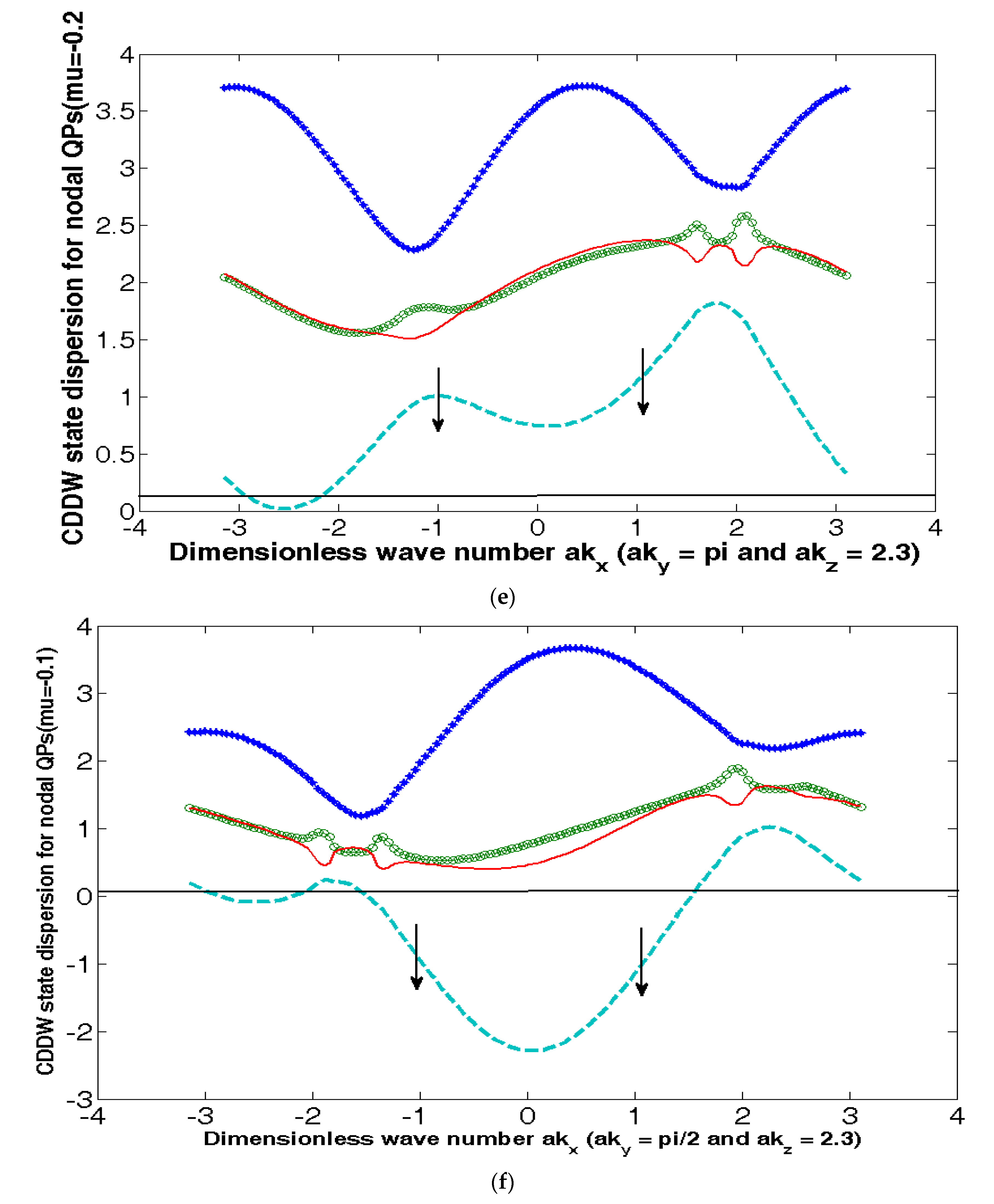The state dispersion is imperfectly nested with the ordering wave vector Q = (Q₁ = ±0.7742 π, Q₂ = ± 0.2258 π), and (Q₁ = ±0.2258 π, Q₂ = ±0.7742 π). We notice that around Γ point (Figure 4a) spin-up quasi-particles (QPs) are conducting, whereas in the anti-nodal/nodal region (Figure 4c,d) spin-down QPs are conducting. The reason for these observations is that the corresponding bands are partially empty. A change in the value of the chemical potential µ by doping does not affect these features as shown in (e) and (f), where µ/t = −0.2 and −0.1, respectively. This is an indicator of the robustness of the system. In Figure 4b, we have contour-plotted the band corresponding to the spin-up QPs in Figure 4a. Thus, the spin-momentum locking is evident. While the nodal region of the momentum space can give rise to a spin- down hole current, the region around the Γ point can give rise to spin-up electron current. The quasiparticle states of opposite spin are to be found in different parts of the Brillouin zone. On the experimental front, recently Vishwanath et al. [7] discovered that Bi2212 has a nontrivial spin texture with the spin-momentum locking. They used a spin- and angle-resolved photoemission spectroscopic technique to unravel this fact. These authors also developed a model to show how this complex pattern could emerge in real and momentum spaces. The key feature is that the layered structure of Bi2212 allows for a spin-momentum locking (SML) in one Cu-O layer of the unit cell that is matched by the opposite spin texture in the other Cu-O layer of the unit cell through the Γ point encirclement in the momentum space representation (see Figure 1 and ref. [7]). This suggests the presence of a strong spin-orbit coupling in Bi2212 like a topological insulator. We shall briefly discuss the encirclement feature below.

The spin texture s(n,k) is defined as the expectation value of a vector operator components S_j = I$2\times 2$ $\otimes {\sigma }_j$ where ${\sigma }_j$ are Pauli matrices on a two dimensional k-grid and ⨂ stands for the tensor product. At k for the state n (or nth band), it is defined as an expectation value s_j(n,k) = ⟨S_j⟩⁽ⁿ⁾ = ⟨n|S_j|n⟩. To calculate s_j(n,k), we need eigenvectors of the Hamiltonian matrix for the eigenvalues $E_j\left(s,\sigma ,k, k_z\right)=$ ${\in }_j\left(s,\sigma ,k\right)\pm {\epsilon }_{\begin{array}{c}{k}_z\\ \end{array}}\left(k\right)$ where ${\in }_j\left(s,\sigma ,k\right) \mathrm{is} \mathrm{given} \mathrm{by} \mathrm{Equation} \left(3\right)$ and ${\epsilon }_{\begin{array}{c}{k}_z\\ \end{array}}$(k) = −ϒ_z(k, s_z(c/2))[(s_x(a) − s_y(a))²/4 + a₀]. These eigenvectors are

$$\left|{\mathsf{\Psi }}_{\mathrm{j}}\rangle \right.={Ϛ}_j{}^{-1}\left(K\right) \left(\begin{array}{c}1\\ {\psi }_2^{\left(j\right)}\left(K\right)\\ {\psi }_3^{\left(j\right)}\left(K\right)\\ {\psi }_4^{\left(j\right)}\left(K\right)\end{array}\right), j=1, 2,3,4, \mathit{K}=\left(k_x,k_y,k_z\right)$$

$${Ϛ}_j\left(K\right)=1+| {\psi }_2^{\left(j\right)}\left(K\right){|}^2+|{\psi }_3^{\left(j\right)}\left(K\right){|}^2+| {\psi }_4^{\left(j\right)}\left(K\right){|}^2,$$

$$\begin{gathered} {\psi }_2^{\left(j\right)}\left(K\right)=\frac{[D_k\left(E_j-{\epsilon }_1\right)\left(E_j-{\epsilon }_2\right)+{\mathsf{\alpha }}_k^{*}{\mathsf{\alpha }}_{k+Q}{D}_k^{†}]}{{\xi }_k^{\left(j\right)}}, \\ {\psi }_3^{\left(j\right)}\left(K\right)=\frac{\left[ {\mathsf{\alpha }}_{k+Q}\left\{{\left(E_j-{\epsilon }_k\right)}^2-|{\alpha }_k {|}^2\right\}-{\mathsf{\alpha }}_{\mathrm{k}}{D}_k^2\right]}{{\xi }_k^{\left(j\right)}}, \end{gathered}$$

$${\psi }_4^{\left(j\right)}\left(K\right)=\frac{\left[\left(E_j-{\epsilon }_{k+Q}\right)\left\{\left(E_j-{\epsilon }_k\right)\left(E_j-{\epsilon }_{k+Q}\right)-|{\alpha }_k {|}^2\right\}-\left(E_j-{\epsilon }_k\right){\left|D_k\right|}^2\right]}{{\xi }_k^{\left(j\right)}},$$

$${\xi }_k={\mathsf{\alpha }}_{\mathrm{k}}{D}_k\left(E_j-{\epsilon }_{k+Q}\right)+{\mathsf{\alpha }}_{k+Q}{D}_k^{†}\left(E_j-{\epsilon }_k\right),$$

$${\epsilon }_1,{\epsilon }_2=\frac{\left({\epsilon }_k+{\epsilon }_{k+Q}\right)}{2}\pm {\left({\epsilon }_k{{}^L}^2+|{\left.D_k\right|}^2\right)}^{\frac{1}{2}} , {\epsilon }_k{}^L=\frac{\left({\epsilon }_k-{\epsilon }_{k+Q}\right)}{2}.$$

(12)

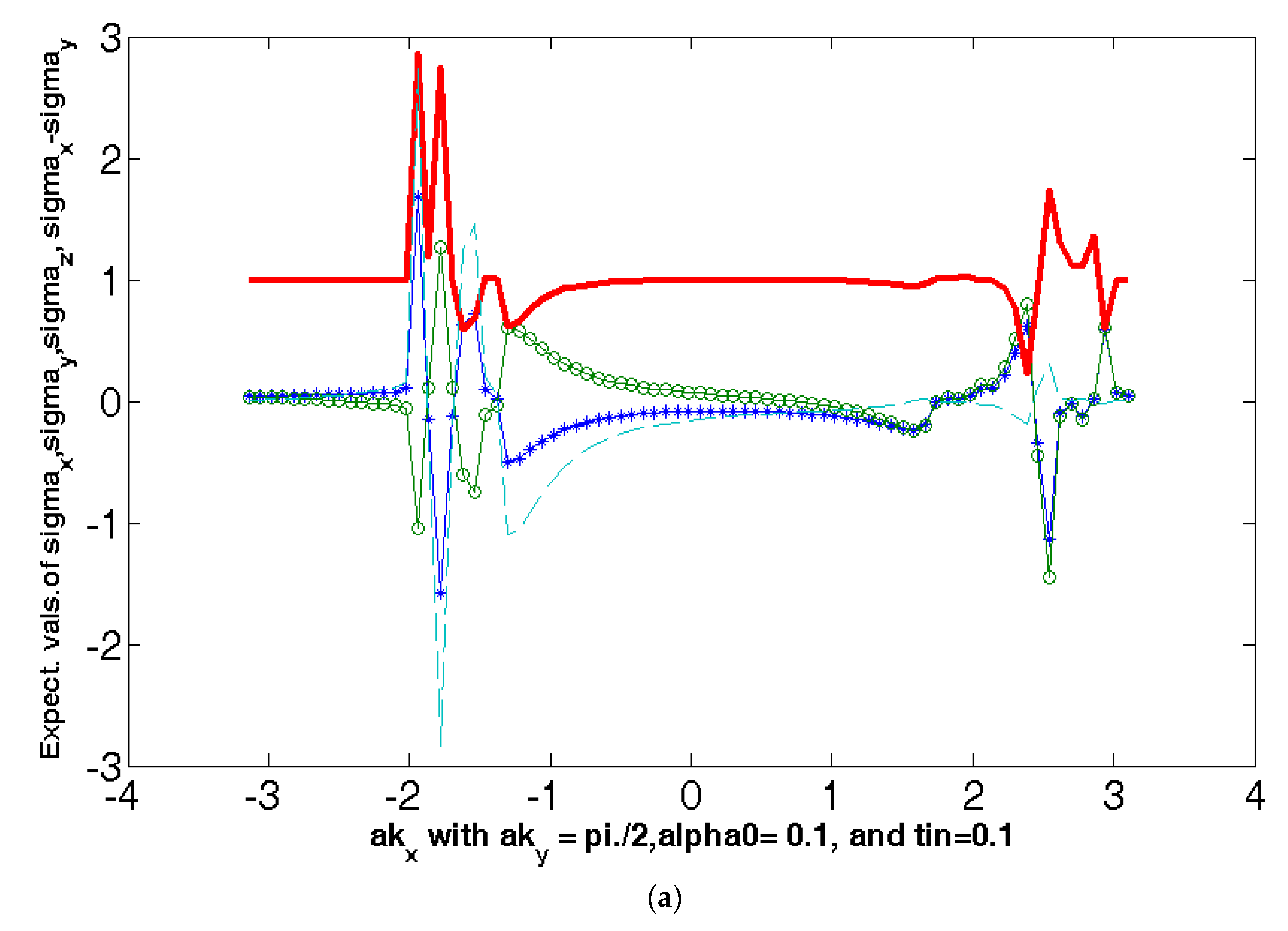
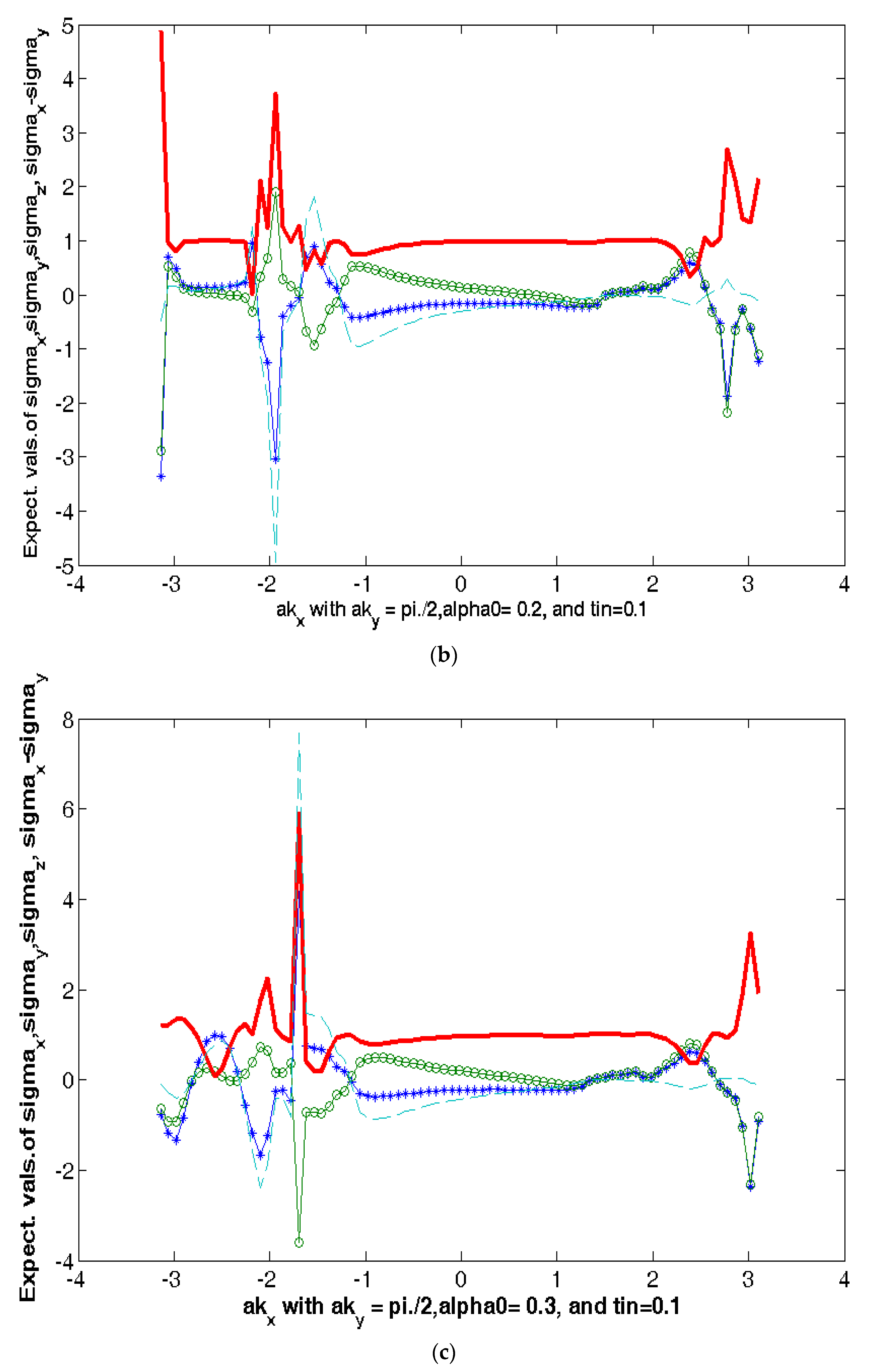
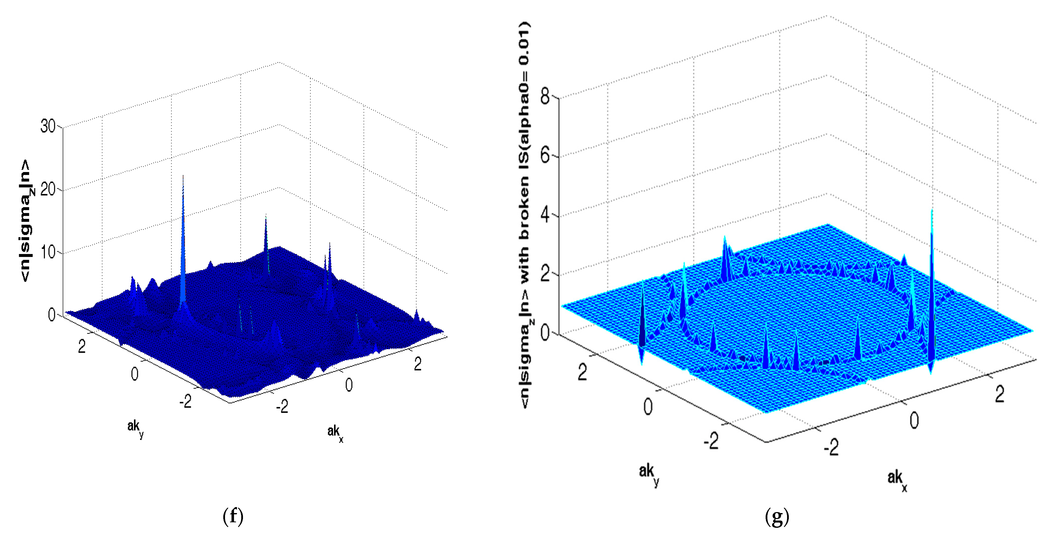
We have calculated expectation value s_j(n,k) considering the eigenvalue $E_j\left(s=-1,\sigma =+1,k\right) \mathrm{corresponding} \mathrm{to} \mathrm{the} \mathrm{bonding} \mathrm{case}.$ The anti-bonding case yields a similar result. The 2D plots of the expectation values are shown in Figure 5. We find that unfailingly, near the nodal point, the expectation values of s_z(n,k) show peaks when the numerical values of the parameter $\frac{{\alpha }_0}{t}=0.1/0.2/0.3 \mathrm{and}$ t_in/t = 0.1/0.15/0.20. Here, the red curve corresponds to the expectation value of s_z(n,k), while the blue (green) curves to the expectation value of s_x(n,k) (s_y(n,k)). The broken (blue) line corresponds to the expectation value of (s_x(n,k) − s_y(n,k)). The numerical values of the additional parameters used in the plots are t = 1, t′/t = −0.28 (hole-doping), t″/t = 0.1, t‴/t = 0.06, t_p/t = 0.3, $\frac{a_0}{t}=0.40, \frac{\mu }{t}$ $=-0.0,$ $∆$₀^(PG) (T)/t = 0.02$, \frac{{\chi }_0}{t}=0.02,$Q₁ = 0.7742 π, Q₂ = 0.2258 π, and $c k_z=2.33$. As shown in the 3D plot of s_z(n,k) in Figure 5f,g, the spike in this quantity is broadly confined to the nodal region. The peaks refer to the highest expectation value of the operator component I_2X2 $\otimes {\sigma }_z$. This simply means that the maximum spin polarization is possible in the nodal region. The Figure 5a–c show that, when the interlayer tunneling t_in is kept fixed, the quantity s_z(n,k) is an increasing function of the RSOC coefficient $\frac{{\alpha }_0}{t}.$ On the other hand, Figure 5a,d,e show that a fixed $\frac{{\alpha }_0}{t},$ s_z(n,k) is a decreasing function of the interlayer tunneling t_in. The origin of this tunability is as follows: A consequence of the so-called inversion symmetry breaking in the direction perpendicular to the two-dimensional plane of the Bi2212 monolayer is the Rashba spin-orbit coupling (RSOC). This can be tuned by gate voltage. As shown in Figure 5g (where we find that the texture almost disappears when RSOC tends towards zero), we notice that the non-trivial spin texture in k-space (spike in the nodal region) is a consequence of RSOC. The texture, therefore, should be tunable by electric field (${\alpha }_0 \mathrm{is} \mathrm{electric} \mathrm{field} \mathrm{dependent})$ and intercalation (conjecturally, this will affect the interlayer tunneling). This is precisely what we find above. Thus, in a large region of the Brillouin zone, the tunable spin textures demonstrate a momentum-selective spin polarization due to RSOC. This has a strong implication for spintronic applications. However, there is a severe hindrance to the potential elbow room of SML to provide resilience in the design of spintronic devices. To explain, we note that in the present system, the spin orientation is regulated by the electron momentum direction. Seemingly, there is a possibility of spin generation and/or detection by controlling the flow of charge or spin currents. In other systems [45,46], where the spin orientation is forced to align perpendicularly to the electron momentum, these have been made in the past. The important point is the manipulation of the spin orientation under the drift, and diffusion makes the task extremely difficult. The synthetic spin-orbit coupling (s-SOC) [47,48,49,50], arising due to Zeeman Hamiltonian involving the position-dependent magnetic field (B₀), may prove to be useful for the spin manipulation. It must be noted that while s-SOC breaks time reversal symmetry (TRS), the intrinsic spin-orbit coupling (i-SOC) comprising of the Rashba and Dresselhaus SOCs (where the former is due to structural inversion asymmetry and the latter is due to bulk inversion asymmetry) are time-reversal symmetric.

We have considered a Bloch Hamiltonian H(k) to describe our system. The Hamiltonian we start with is nearly the same as that put forward by Das Sarma et al. [5,6] when we do not consider RSOC. Two important symmetries one needs to consider here are time reversal symmetry (TRS) and inversion symmetry (IS). The Das Sarma Hamiltonian is TRS broken. The IS is protected as long as the ordering wave vector Q = (±π, ±π). For Q $\ne$ (±π, ±π), the IS protection is lost, even in the absence of the Rashba term. Suppose the eigenvectors corresponding to the energy eigenvalues of H(k) are denoted by $u^{\left(n\right)}\left(k\right),$ where n is a band index. Suppose $u^{\left(n\right)}\left(k\right)$ is a Bloch state eigen wavefunction. The Berry curvature (BC) is defined as

$${\Omega }_{\mathrm{xy}}^{\left(n\right)}\left(k\right)=i\langle {\partial }_{k_x}{u}^{\left(n\right)}\left(\mathrm{k}\right)|{\partial }_{k_y}{u}^{\left(n\right)}\left(\mathrm{k}\right)\rangle -i\langle {\partial }_{k_y}{u}^{\left(n\right)}\left(\mathrm{k}\right)|{\partial }_{k_x}{u}^{\left(n\right)}\left(\mathrm{k}\right)\rangle$$

(13)

The inversion symmetry implies ${\Omega }_{\mathrm{xy}}^{\left(n\right)}\left(k\right)={\Omega }_{\mathrm{xy}}^{\left(n\right)}\left(-k\right),$ and TRS implies ${\Omega }_{\mathrm{xy}}^{\left(n\right)}\left(k\right)=-{\Omega }_{\mathrm{xy}}^{\left(n\right)}\left(-k\right) .$ Thus, for a system which is both TRS and IS compliant, ${\Omega }_{\mathrm{xy}}^{\left(n\right)}\left(k\right) \equiv 0$. This means that in order to study the possible quantum anomalous Hall (QAH) effect starting from the present DDW ordered TRS (IS) compliant (noncompliant) system of Bi2212 bilayer we need to have broken TRS which yields non-zero Berry curvature (BC). A non-zero BC is very much required to obtain anomalous Hall conductivity $\left({\sigma }_{xy}\right)$ and to show that ${\sigma }_{xy}$ is quantized in the case of an insulator. Although the Dirac model approach has its limitations, it is nevertheless useful in understanding the topological properties of realistic materials. Since the intrinsic QAH effect can be expressed in terms of BC, it is therefore an intrinsic quantum-mechanical property of a perfect crystal. An extrinsic mechanism, skew scattering from disorder, tends to dominate the QAH effect in highly conductive ferromagnets. Since bands close to the Fermi level correspond to those of chiral/helical fermions (Dirac-like model), as already stated, we consider the following energy eigenvalues (derivable from (1) assuming long wavelength limit): ${ϵ}_{k,1} \approx {\epsilon }_{k }– \sqrt{M^2+{\alpha }_0^2({\left(a{k}_x\right)}^2+\left(a{k}_y{)}^2\right)+O\left({Ϛ}^2\right)},\mathrm{and}$ ${ϵ}_{k,2} \approx -{\mathsf{\epsilon }}_{\mathrm{k} }+\sqrt{M^2+{\alpha }_0^2({\left(ax+a{Q}_1\right)}^2+{\left(ay+a{Q}_2\right)}^2)+O\left({Ϛ}^2\right)},$ where $Ϛ=(\frac{{\chi }_0}{2}$) $\left(a{k}_x\right)\left(a{k}_y\right)+\left(\frac{i}{4}\right)∆$₀^(PG) (T)(${\left(a{k}_x\right)}^2+{\left(a{k}_y\right)}^2)$. 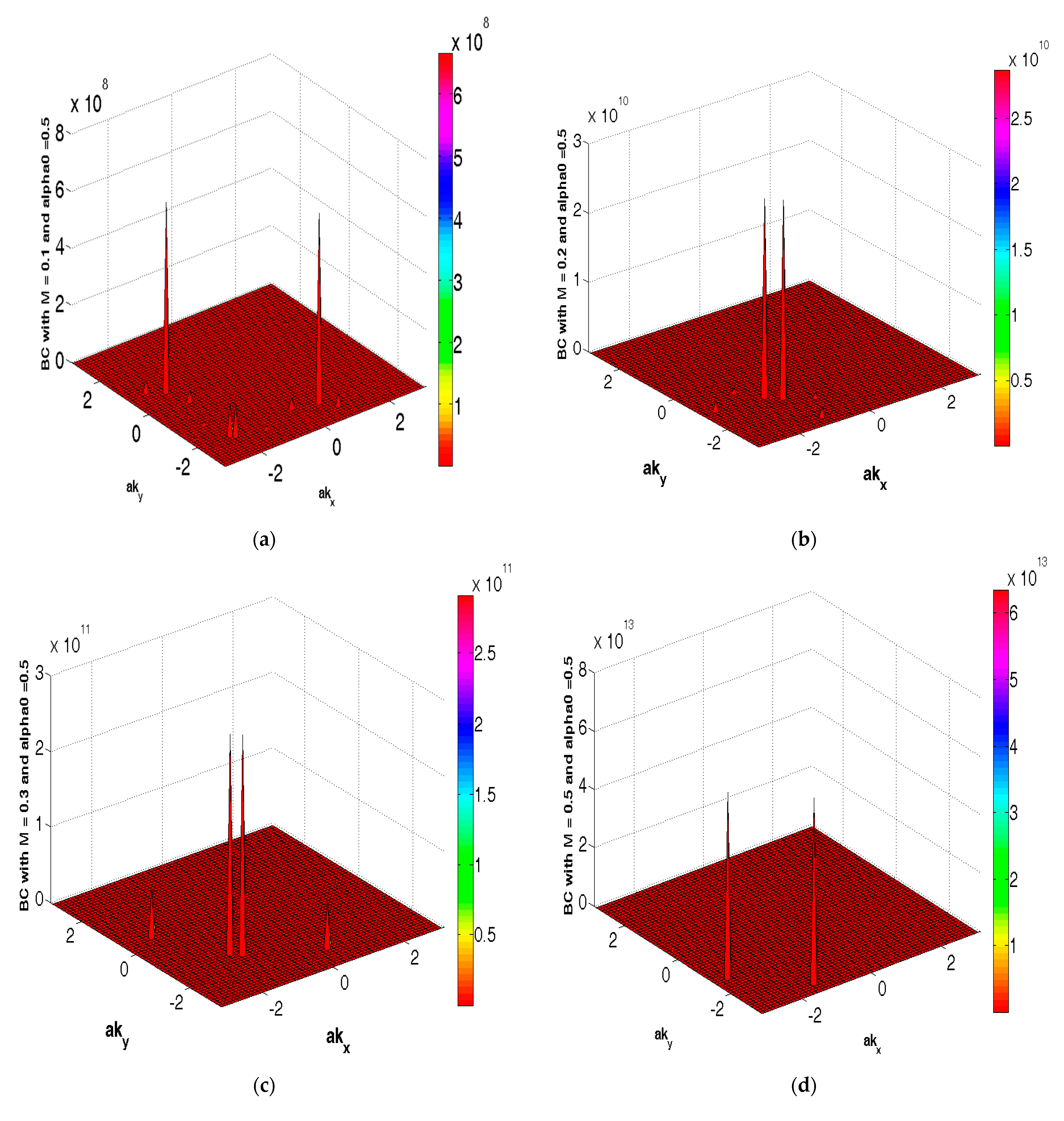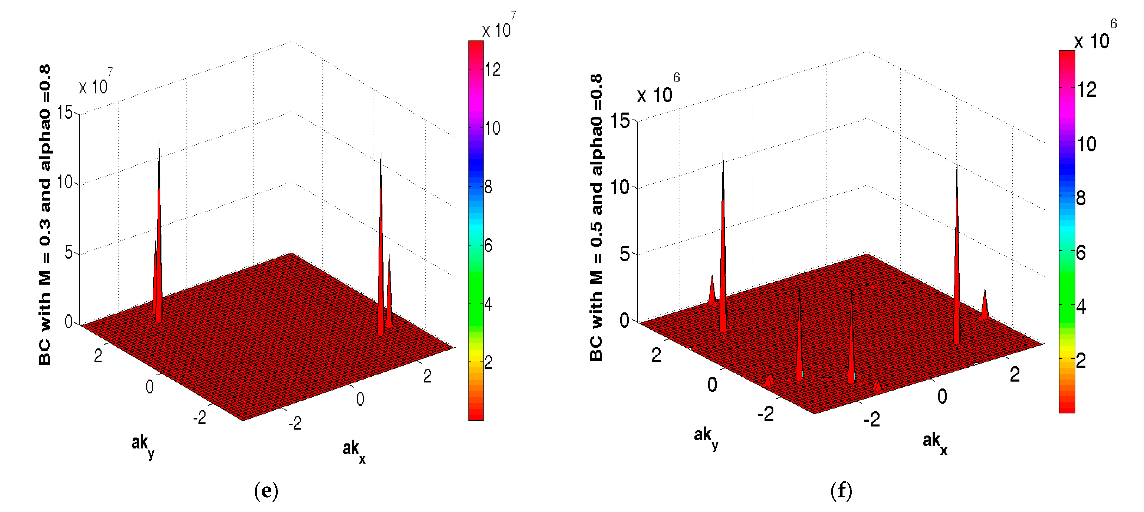Upon using the formula in Equation (13) we find the BC (${\Omega }_{\mathrm{xy}}\left(k\right))$ as ${\Omega }_{\mathrm{xy}}\left(k\right)={\Upsilon }_{\mathrm{x}, \mathrm{y}}\left(k\right)+{\Upsilon }_{{\mathrm{x}}_1,{\mathrm{y}}_1}\left(k\right)$ where

$${\Upsilon }_{\mathrm{x},\mathrm{y}}\left(k\right)=\frac{4{\alpha }_0^{2}xy\left(\frac{\partial {ϵ}_1}{\partial x}\right)\left(\frac{\partial {ϵ}_1}{\partial y}\right)}{{(({ϵ}_1-{\mathsf{\epsilon }}_{\mathrm{k} })+M)}^4}-\frac{2{\alpha }_0^2}{{(({ϵ}_1-{\mathsf{\epsilon }}_{\mathrm{k} })+M)}^2}-\frac{2{\alpha }_0^2\left\{x\left(\frac{\partial {ϵ}_1}{\partial x}\right)+y\left(\frac{\partial {ϵ}_1}{\partial y}\right)\right\}}{{(({ϵ}_1-{\mathsf{\epsilon }}_{\mathrm{k} })+M)}^3},$$

(14)

and ${\Upsilon }_{{\mathrm{x}}_1,{\mathrm{y}}_1}={\Upsilon }_{\mathrm{x}, \mathrm{y}}({ϵ}_1\to {ϵ}_2,$x$\to x_1,y\to y_1).$ The plots of BC, as a function of ($a{k}_{\mathrm{x}},a{k}_{\mathrm{y}}) \mathrm{with}$ the chemical potential µ $=-$0.5, are shown in Figure 6. In Figure 6a–f, the common feature is the spikes in certain regions of the Brilloin zone close to the nodal points. The parameter values in (a) M/t = 0.1, and $\frac{{\alpha }_0}{t}=0.5, \left(\mathrm{b}\right)M/t=0.2,\mathrm{and} \frac{{\alpha }_0}{t}=0.5,$ (c) M/t = 0.3, and $\frac{{\alpha }_0}{t}=0.5, \left(d\right)\frac{M}{t}=0.5,\mathrm{and} \frac{{\alpha }_0}{t}=0.5, \left(\mathrm{e}\right)\frac{M}{t}=0.3,\mathrm{and} \frac{{\alpha }_0}{t}=0.8, \mathrm{and} \left(\mathrm{f}\right)\frac{M}{t}=0.5,\mathrm{and} \frac{{\alpha }_0}{t}=0.8$. The other parameter values are t = 1, t′/t = −0.28 (hole-doping), t″/t = 0.1, t‴/t = 0.06, t_p/t = 0.30, t_m/t = 0.10, $∆$₀^(PG) (T)/t = 0.40$, \frac{a_0}{t}=0.20, \frac{{\chi }_0}{t}=0.1, \mathrm{and} c{k}_z=2.33$. As the colorbars suggest, at a given $\frac{{\alpha }_0 }{t}=0.5,$ as the exchange field increases, the peaks in BC increases form value of O(10⁸) to value of O(10¹³). However, for $\frac{{\alpha }_0 }{t}=0.8,$ not only do the peaks value of O(10⁷) for M/t = 0.3 go to a higher order of magnitude for the increase in M/t, there is the proliferation of spikes, as well with the increase in the exchange field. These are tentative conclusions, as we have not dealt with a large number of cases. In order to explain what these peaks signify, we refer to the Chern number C (TKNN invariant) we shall encounter below in the calculation of Hall conductivity. The invariant, in fact, allows us to properly define the electric polarization as a topological quantity (see Appendix A). The Berry phase is given by this invariant. As regards the Berry connection ${\mathit{A}}_{\mathit{n}}$ and Berry curvature ${\Omega }^{\left(n\right)}\left(\mathit{k}\right)$ ($\mathrm{where} {\nabla }_{\mathit{k}}\times$ ${\mathit{A}}_{\mathit{n}}\left(\mathit{k}\right)={\Omega }^{\left(n\right)}\left(\mathit{k}\right)),$ they can be viewed as a local gauge potential and gauge field associated with the Berry phase (or geometric phase, or Pancharatnam phase), respectively. The peaks therefore signify spiking values of the gauge field associated with the Pancharatnam phase.

The Chern number C, which is an integer, is given by C = 2 ∫∫_BZΣ_n ${\Omega }_{xy}^{\left(n\right)}\left(k\right)\frac{d^{2}k}{{\left(2\pi \right)}^2}$. Here, ${\Omega }_{xy}^{\left(n\right)}\left(k\right) is \mathrm{the} \mathrm{Berry}-\mathrm{curvature} \left(\mathrm{BC}\right) \mathrm{component} \mathrm{along} \mathrm{z} \mathrm{direction}, \int \int$ _BZ denotes an integral over the entire Brillouin zone (BZ), and the sum is over occupied bands. The Hall conductivity σ_xy in a band insulator is related to the Chern number C by σ_xy = (e²/2h) C. The sign of the Hall contribution is determined by the relative signs of BCs. In the case when the system is insulator (that is, when the chemical potential lies within the band gap), C $=\left(\frac{1}{2\mathsf{\pi }}\right)\oint {\Sigma }_{n}d\mathit{k}· {\mathit{A}}_{\mathit{n}}$ is an integer. The closed loop corresponds to the encirclement of the Brillouin zone boundary. The anomalous Hall conductivity is then quantized. The reason is because of the single-valued nature of the wave function, and its change in the phase factor after encircling the Brillouin zone boundary can only be an integer multiple of 2π or 2 π m, which means C can only assume an integer value. Hence, σ_xy is quantized to integer multiples of e²/h. The TKNN invariant plays the role of the topological invariant of the quantum Hall system.

Upon referring to Figure 4, we find that the fermi energy does not lie within the band gap. Therefore, we need to calculate C analytically and examine how close is it to an integer. This quantity C or the Hall conductivity itself, in a semi-classical approach, is given by

$${\sigma }_{xy}=\int \left(\frac{e^2}{\hslash } \right){{\displaystyle \sum }}_{\mathrm{n}}\frac{d^{2}k}{{\left(2\pi \right)}^2} f_n\left(k\right) {\Omega }_{\mathrm{xy}}^{\left(n\right)}\left(k\right)$$

(15)

where $f_n\left(k\right) \mathrm{is} \mathrm{the} \mathrm{Fermi} \mathrm{occupation} \mathrm{function} \mathrm{and} {\Omega }_{\mathrm{xy}}^{\left(n\right)}\left(k\right)$ is the z-component of the BC.

In fact, most of the conventional approaches to the electronic transport in solids are based on the very general linear response theory of Kubo [51]. The Kubo formula for the anomalous Hall conductivity (AHC) in the static limit for disorder-free non-interacting electrons is given by the $\widehat{v} \mathrm{which} \mathrm{is} \mathrm{the} \mathrm{velocity} \mathrm{operator}, \mathrm{and} {\in }_n\left(k\right)$ which are the eigenvalues of the surface state Hamiltonian $\widehat{H}$ in QAH state. In momentum eigen basis, the velocity operator is given by $\widehat{v}=\left(\frac{1}{\hslash }\right)\frac{\partial \widehat{H}}{\partial k}$. The Kubo approach also leads to the same expression as (15). We have already calculated BC, in the long wavelength limit, in Equation (14). The limit ensures that bands close to the Fermi level correspond to those of chiral/helical fermions (Dirac-like model). As one can see from (15), to obtain the Hall conductivity, momentum space integration is necessary. For this purpose, we have used the Matlab package. Here, we first divide the Brillouin zone into finite number of rectangular patches. We next determine the numerical values corresponding to each of these patches of the momentum-dependent density and sum these values. The sum is then divided by the number of patches. We find, for example with M/t = 0.5, C = 0.7488 sgn(M/t). This is quite satisfactory. The reason for not obtaining an integer, as we surmise, rests upon the following: The Hall conductivity σ_xy cannot be determined as such from the 2D Dirac model, since (15) requires an integral over the whole BZ, as we have seen above. The integral is outside the Dirac model’s range of validity. To circumvent the problem, one may possibly choose a momentum space cut-off small compared to the size of BZ and large enough to capture nearly all the contributions to BC integral. This will be within the range of validity of the 2D Dirac model.

4. Discussion

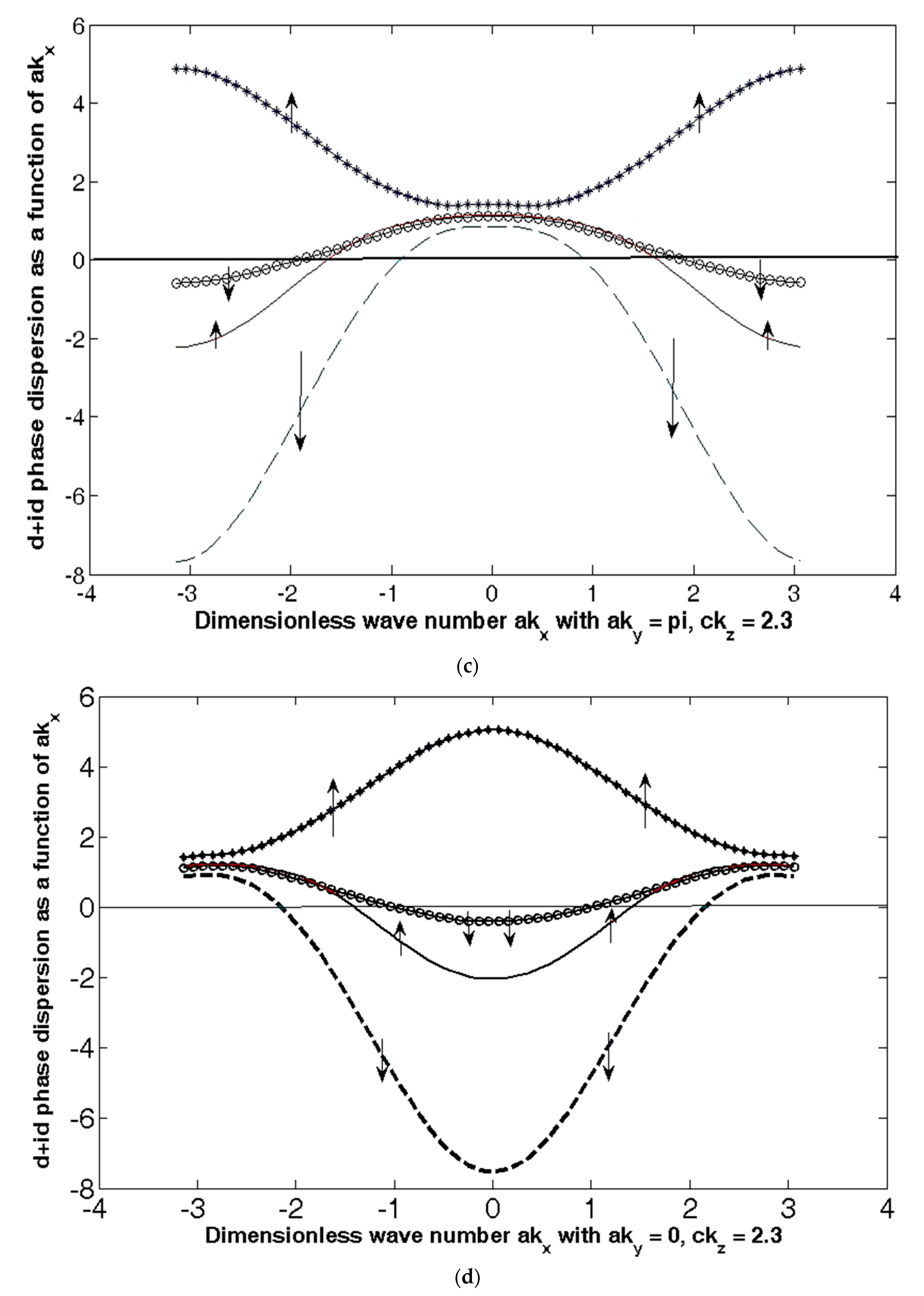
We have added in the Rashba term by hand. Here, we provide a sufficiently strong supporting argument from band structure calculation as follows. In fact, there is a lack of evidence of the spin-momentum locking when the Rashba coupling is totally absent. This necessitates its inclusion. To justify this statement, we show the plots of the energy eigen-values in Equation (1) in the nodal and anti-nodal regions, which are shown in Figure 7b–d above in the absence of the Rashba coupling. The numerical values of the parameters used are t = 1, t′/t = −0.28 (hole-doping), t″/t = 0.1, t‴/t = 0.06, t_b/t = 0.3, t_z/t = 0.1, $\frac{{\alpha }_0}{t}=0, \frac{{\alpha }_1}{t}=0,\frac{{\chi }_0}{t}$ = 0.44, $\frac{{∆}_0^{PG}}{t}=0.2, \mathrm{and} a_0=0.4$. In Figure 7a, we have a plot of quasi-particle excitation (QP) spectrum in z-direction given by ${\epsilon }_{\begin{array}{c}{k}_z\\ \end{array}}$(k) = −ϒ_z(k, s_z(c/2))[(s_x(a) − s_y(a))²/4 + a₀], given above as a function of dimensionless momentum $a{k}_z$ at the nodal point. In Figure 7b–d, we have plots of the excitation spectrum in the CDDW state as a function of $a{k}_x \mathrm{with} a{k}_z=2.3$. In Figure 7b, the plot is for $a{k}_y=\frac{\pi }{2}.$ We find that only the spin-down valence band is partially empty. In Figure 7c,d, respectively, the plot is for $a{k}_y=\pi$ and $a{k}_y=0$. We find that only the spin-up conduction band is completely full, whereas the rest of them are partially empty. Thus, while the nodal region of the momentum space can give rise to a spin-down hole current, no other region can give rise to spin-polarization or spin-current. We conclude that the spin-momentum locking (SML) is not evident in the absence of the Rashba coupling in Bi2212 bilayer system. This is a very strong argument in favor of the inclusion of the Rashba coupling for the problem in hand. The coupling has novel upshot as discovered by Gotlieb et al. [7]. They found that Bi2212 has a nontrivial spin texture with the spin-momentum locking. They used spin- and angle-resolved photoemission spectroscopic (SARPES) technology to unravel this fact. They also developed a model to show how this complex pattern could emerge in real and momentum spaces. The key feature is that the layered structure of Bi2212 allows for a spin-momentum locking in one Cu-O layer of the unit cell that is matched by the opposite spin texture in the other Cu-O layer of the unit cell, as shown in Figure 1, through the Γ point encirclement in momentum space representation. This type of spin-momentum ordering is hidden from other experimental techniques, except SARPES [7]. A similar figure is also displayed in Figure 5f. As shown in the plot of the texture s_z(n,k) in this figure, the spike in s_z(n,k) is broadly confined to the nodal region, and there is encirclement of Γ point.

The Rashba spin-orbit coupling (RSOC), which can be tuned by gate voltage (or, electrostatic doping), is a consequence of the so-called structural inversion symmetry. On the other hand, SOC linked to the bulk inversion symmetry is referred to as the Dresselhaus coupling (D-SOC). Here, both k-linear and k-cubed terms are involved [52]. The linear term is given by: β₀ (σ_x sin (k_xa) $-$ σ_y sin (k_ya)) where β₀ is the Dresselhauss spin-orbit coefficient [53,54]. The cubic term, on the other hand, is γ₀ (σ_x (k_ya)² (k_xa) $-$ σ_y (k_xa)² (k_ya)), where γ₀ is the Dresselhauss spin-orbit coefficient. It is well-known [53,54] that the coexistence of Rashba and Dresselhaus contributions is possible in a two-dimensional spin-orbit coupled system without inversion symmetry. Therefore, one needs to include the D-SOC term in the Hamiltonian to observe the effects of cubic term in SML, QSH, and QAH effects. In fact, much remains to be understood and explored in this field. The model one wishes to consider might be realized with cold atoms. The Rashba and Dresselhaus spin-orbit coupling can be realized in cold atoms [55,56] in an optical lattice experimentally. We have addressed above the question of “what is the necessity of breaking inversion symmetry (IS)”. In this context, one may note further that in their seminal work, Zhang et al. [57] have demonstrated that the lack of the local inversion symmetry at atomic sites leads to hidden spin polarization completely determined by the site-dependent orbital angular momentum, even in centrosymmetric crystals. This was an outcome of the first-principles calculations by the authors. Usually, the reason behind this is the orbital magnetization being more important than the spin magnetization, i.e., the spin–orbit coupling (SOC) is weak, such as in a transition metal dichalcogenide (TMD) MoS₂. Additionally, Baidya et al. [58] had also explored the important role of orbital polarization in QAH phases. A comparison with DFT calculation led these authors to the conclusion that the effect of such terms is smaller.

The QSH effect shown by the Bi2212 bilayer system under consideration is related to the formation of the Moir’e patterns [59,60] under a relative rotation between the two CuO₂ layers in the bilayer system. To explain, as the creation of the Moir’e landscape gives rise to the realizations of an external non-Abelian gauge field, which couples the motional states of the particles to their spins (internal degree of freedom), the field can be regarded as an extension of RSOC in some sense. The quantum spin Hall effect is, therefore, tunable by this field. However, since the Moir’e electron system is generally described by (massless) Dirac fermions on each layer, coupled with a position-dependent interlayer hopping amplitude, the access to this tuneability does not seem to be possible. As discussed in Appendix A, our system comprises of ‘helical (massive) liquids’ in the quasi-2D geometry. Nonetheless, the problem needs a close inspection before concluding that the ‘mass’ factor excludes the formation of the Moir’e patterns [59,60].

In summary, we have, possibly for the first time, found that a DDW ordered [1,2,3,4] PG state model of Bi2212 bilayer, which involves the Rashba spin-orbit coupling, can display QSH effect. On a quick side note, it may be mentioned that the classical counterpart of QSH effect is accessible in optical systems [61]. For example, Kapitanova et al. [62] have experimentally shown that, based on the optical spin-orbit locking phenomenon, photonic spin Hall effect is possible in hyperbolic meta materials (HMM). This important class of artificial anisotropic materials have a unique ability to control interactions between electromagnetic waves and matter. Upon coming back to our model Hamiltonian with DDW/CDDW order, we note that the model with DDW order [1,2,3,4] describes the low energy physics of a class of helical fermionic liquid in our spin-orbit system. We also predict the existence of QAH effect in the context of an extension of the DDW model, viz. chiral DDW ordered state [5,6] with magnetic impurities. The issue of the robustness of QSH and QAH systems with change in the chemical potential is addressed graphically in Figure 2c,d and Figure 4e,f, respectively. The robustness of the existence of the edge state and tunnelling between edge states in a SO coupled system is an important part of the problem. We write: The surface of the system has states, which come in an odd number of Kramers’ doublets, as in Figure 2. Macroscopically, these counter-clockwise/clockwise circling states are carrying spin down/up, or vice versa, depending on the orientation of the magnetic field ${\mathit{B}}_{{\alpha }_0}=\left(\frac{2{\alpha }_0}{g{\mu }_B}\right) \left(a\mathit{k}\times \widehat{\mathit{z} }\right)$ that enters the spin-orbit interaction. The edge states appear as a consequence of the cyclotron orbits induced by the magnetic field, which are naturally truncated at the physical boundary of the sample. The energy levels of the counter-propagating edge state bands cross at particular points in the Brillouin zone due to TRS, and the spectrum cannot be continuously deformed into that of an ordinary band insulator. In this sense, an insulator realizes a topologically nontrivial state of matter. The QSH and QAH systems have potential technological applications in spintronics. There are plenty of future challenges and opportunities in this rapidly evolving area.