Distributed Optimal Placement Generators in a Medium Voltage Redial Feeder

Abstract

Distributed generation (DG) is an important issue for distribution networks for power loss improvement. However, the location and size of generators remain a challenge for existing techniques. This work investigates the optimal placement of a distributed generator on a medium voltage radial feeder. Simulated annealing optimisation is used to find an optimal bus of connecting a distributed generator variable-spider. The optimisation technique is then applied to a power flow Matlab program that incorporates the Newton–Raphson method. DigSilent PowerFactory simulations software is used to validate the results that are obtained from the Matlab program. The results indicate that the optimal bus for a 14-bus radial feeder loaded at 5 MVA while using a 1.5 MW DG is bus 11. This is because connecting the distributed generator at bus 11 resulted in maximum loss reduction on the feeder. The Matlab tool proposed in this study can be used to find the optimal bus where a distributed generator can be connected to a medium voltage radial feeder, thereby improving power quality and fulfilling load demand with minimal size to make the system economical.

1. Introduction

Energy resources can be classified into three categories, namely, fossil fuels, nuclear energy and renewable energy [1]. Fossil fuel energy is energy that is generated from the use of hydrocarbons (oil, coal and natural gas) that form from dead organisms such as plants and animals that were buried millions of years ago [2,3,4]. Approximately 66% of electricity generated worldwide comes from fossil fuels [5]. Nuclear energy is energy that is released from a nuclear reaction that takes place through fission or fusion [6]. By the end of 2002, there were 414 nuclear power plants, which were supplying about 16% of the global electricity generated [7]. Nuclear energy is used as support energy in most countries [7]. The expansion in usage of nuclear energy relies on reactor technology innovation, which should ensure that nuclear security and proper disposal of nuclear wastes are in place [7]. Renewable energy is defined as energy that is generated from renewable natural resources such as wind, sunlight, geothermal heat, water and biomass [8].

There are five types of renewable energy technologies, namely, biomass, hydropower, solar, wind and tidal waves. Biomass is defined as the energy generated from the combustion of organic materials. Examples of organic materials are wood chunks and debris, human and animal wastes, dedicated crops such as wheat and sugar cane and liquefied oil derived from biomass. During combustion, the organic materials are used to burn water into steam, which is used to drive a turbine that is coupled to a generator. Hydropower is considered one of the biggest renewable energy technologies [9,10]. In 2006, hydropower stations were contributing approximately 15% of the global electricity [11,12,13,14,15].

This kind of technology converts the potential energy of water into mechanical energy. The water flows from a reservoir down a penstock using gravity. The water then hits the fins of a turbine, which is coupled to a generator, installed in the penstock. The water from the turbine is allowed to flow downstream of the dam to the river. Solar power is defined as the ability to convert sunlight into electricity [16,17,18]. Two methods are used to convert sunlight into electricity, and they are photovoltaic (PV) cells and concentrated solar power (CSP) [17,18]. PV cells are known as direct because the electricity is generated by them. With CSP, mirrors and lenses concentrate the sunlight to a collector, which then transfers the heat from the sun to a heat transfer fluid. The fluid is then used for generating electricity. The heat can also be used for other industrial processing applications as well as space heating [17,18].

There are four types of CSP technologies: parabolic trough, fresnel reflector, central receiver and parabolic dish [18,19]. Currently, South Africa does not have wind farms that are commercially operational [20,21]. The first commercial wind farm, called Sere, is currently under construction in the Western Cape Province and is expected to be fully operational by halfway through the year 2022 and commercially available by the end of 2022. The wind farm is expected to deliver 100 MW of power [21]. A wind farm consists of wind turbines that are connected to give one output, e.g., 100 MW [18,22].

The major components of a wind turbine are the rotor, fins, low-speed and high-speed shafts, gearbox, generator, controller, anemometer, wind vane and tower [18,23]. When the wind blows, it hits the fins of the rotor and then the rotor rotates. The rotor is attached to the low-speed shaft, so that when the rotor rotates the shaft also rotates, causing the gearbox system to turn. The high-speed shaft is attached between the gearbox system and the generator. When the high-speed shaft rotates, the generator rotates as well, thus generating electricity [17,18,23].

Tidal power is defined as the form of hydropower that converts the energy of ocean tides into a useful form of electrical energy [24,25]. The gravitational force of the moon and sun causes the motion of the ocean. Since the moon is closer to the earth than the sun is, the motion of the ocean is mostly due to the moon. When such motions occur, waves called tides are formed [17,24]. A Matlab-Simulink model has been used to simulate a tidal current turbine [26].

There are two commercially available methods of generating tidal power, and they are tidal stream generator and tidal barrage [17,24]. A tidal stream generator is a generator that generates electricity due to the flow of tidal water through it [17,24]. These generators are mounted in the water of the ocean, and the motion of the ocean tides causes the blades of the generators to rotate, thus causing the generator to rotate and generate electricity [17,24]. This kind of tidal generator resembles that of a wind turbine. The tidal barrage method employs a technique that is similar to that used in a hydropower station [17,24]. In this method, sluice gates are opened for the tides to fill up a basin of a barrage. The water is kept in the basin until the tides have created a suitable head. The water is then released from the basin to the sea via turbines until the tides return. Electricity is then generated by the generators that are coupled to the turbines [17,24].

Two types of rotating generators are used for wind turbines: synchronous generators and induction generators [18]. The induction generators can be classified as fixed-speed and variable-speed [17,18]. The induction generator that is used most is a double-fed induction generator (DFIG). It is mostly used in applications such as wind turbines that require variable-speed control [18].

Africa and the Middle East have the best solar irradiance [1]. Most areas in South Africa have an average of more than 2500 sunshine hours per year and an average solar irradiance of between 4.5 and 6.5 kWh/m² in one day [27]. The annual 24-h global solar irradiance average is about 220 W/m² for South Africa, compared to 150 W/m² for the USA and 100 W/m² for Europe [27]. According to the South African Weather Service [28], there are two provinces in South Africa, namely, Eastern Cape and Western Cape, that have the most winds.

The Western Cape’s Cape Point experiences winds of about 14 m/s on annual average, with 42% of the winds having a wind speed greater than 8 m/s [28]. In Cape Town, winds with a speed greater than 8 m/s occur on 18.1% days of the year and the average annual speed of the wind is 1.6 m/s. In the Eastern Cape, winds of speeds of about 1.6 m/s annual average are experienced in Port Elizabeth; wind speeds higher than 8 m/s are experienced on 20.2% days of the year [28].

In South Africa, the place that is considered to be very hot is Letaba in Limpopo Province. It has a mean annual temperature and average annual maximum temperature of 23.3 °C and 35 °C, respectively [28]. The coldest place in South Africa is Buffelsfontein in the Eastern Cape; this place has a mean annual temperature and an average annual high and low temperatures of 11.3 °C and 2.8 °C, respectively [28].

Increasing usage of distributed generation by power utility companies means increasing the construction of renewable energy farms, e.g., PV farms and wind turbine farms. The community where such farms are constructed will have jobs during the construction and also during maintenance and operation [22]. The Sere Wind Farm that is currently under construction in the Western Cape employed about 400 people from the Matzikama community and its surroundings [22]. The supplier of the farm equipment will also create jobs. The persons employed due to the existence of renewable generation will also contribute to the economy of the country, South Africa in this case.

One disadvantage during the construction of renewable energy generators is that there might be traffic around the towns when the vehicles carrying site equipment pass by. Wind turbines make noise when they are operational, and this might affect surrounding communities [29].

Eskom’s (a South African utility company) power generation is currently dominated by coal power [22]. The production of power from coal is limited to its reserves, and it is also an environmental issue. Coal is a source of carbon dioxide and other gases; carbon dioxide contributes to global warming, and the other gases lead to acid rains [30]. As part of the initiation by the South African government to combat carbon dioxide emissions, it was expected that 10,000 GWh of energy should be from renewable energy by the year 2013 [22].

Nuclear energy is considered to have minimal negative effects on the environment, but poor disposal of its wastes can have severe consequences on the environment [31]. Even though renewable energy is known to be clean energy, it also affects the environment, e.g., when constructing a hydropower station, a dam is built, which then starves natural vegetation, fishes, etc. downstream of the dam [32]. The same is true for tidal generators, which affect the lives of animals such as fish that live in water [25].

Photovoltaic (PV) cells are considered as clean without any emissions during their operation, but the chemicals that are used during their manufacturing can have severe consequences on the environment [33]. Proper disposal of solar panels is very important at the end of their life.

Independent power producers apply to Eskom to have their distributed generators (e.g., wind, solar) connected to the Eskom power system grid. Such connections are done both on the medium voltage (MV) network and on the low voltage (LV) network of the distribution network. Power from distributed generations depends on the availability of solar, wind, etc., and this can affect the power system stability [34]. The traditional power system always assumed that power flow is from generation to distribution, but with the introduction of distributed generations, power can also be generated from distribution to generation; this, therefore, changes the configuration of the power system network and so is its expected operation [34].

The major contribution of this paper is an investigation of the optimal placement of a distributed generator on a medium voltage radial feeder. The research investigates the impact of connecting distributed generators to a power system to find the optimal location and sizes of such generators. This is meant to help reduce power losses while maintaining a voltage profile within acceptable limits. The research will therefore assist power utility companies, such as Eskom, Municipalities and independent power producers (IPPs) in South Africa and beyond to be aware of the impact of connecting distributed generation into their grid and to plan an optimal location for their distributed generation farms for maximum generation. This will help them to avoid building power farms where they will get minimum generation or where they will get maximum generation but are too far from a distribution network.

The remainder of the paper is organised as follows. Section 2 presents the fundamental concepts on optimal placement of distributed generators, and Section 3 explains the study methodology. Section 4 shows our experiments on large-scale real power datasets. Section 5 discusses the results of our experimentation. We draw our conclusions in Section 6.

2. Related Work

Optimal placement of distributed generators requires one to understand the mathematics of optimisation. The optimisation is defined as the act of achieving the best possible results in any given set of circumstances [35,36]. The best results can be obtained by a function of several variables to be maximised or minimised subject to one or more constraints. Two types of constraints are defined, namely, equalities and inequalities [36].

Optimisation techniques are applied in statistics, aerodynamics, chemical engineering, operational research, electrical network design, optimum design of control systems, inventory control, design of water resource systems and many other applications [35,36].

Optimisation methods are divided into traditional and modern methods. The traditional method includes linear programming, nonlinear programming, quadratic programming, geometric programming, integer programming and dynamic programming, whereas the modern optimisation methods are genetic programming, ant colony optimisation, particle swarm optimisation and simulated annealing optimisation. Modern optimisation methods have developed in recent years and are conceptually different from traditional mathematical programming techniques. Most of these methods are based on certain characteristics and behaviours of biological, molecular, swam of insects and neurobiological systems [35].

2.1. Optimisation Techniques

2.1.1. Linear Programming

In linear programming, the objective function and constraints are linear functions of the decision variables [35,36]. The constraints are in the form of equalities or inequalities [35]. The linear programming problem may be represented in two ways, namely, matrix form and scalar form [35]. A linear programming problem with a minimisation objective function can be converted to a maximisation problem by multiplying the objective function by −1, whereas the inequality of a constraint can be converted to equality by simply adding a variable if the inequality is “less than or equal to” or subtracting a variable if the inequality is “greater than or equal to” [35]. For a system with m equality constraints and n variables, the number of basic solutions is given by [35,37]

$$\left(\begin{array}{l}n\\ m\end{array}\right)=\frac{n!}{(n-m)!m!}$$

(1)

For large values of n and m, it becomes impractical to find all the basic solutions. A basic solution is therefore found by equating all (n − m) variables to zero. A method called the Simplex Method is best known for handling such applications and is one of the most used methods in numerical computing [35].

2.1.2. Nonlinear Programming

A nonlinear programming problem is an optimisation problem whose objective function is nonlinear [35,36]. Given an optimisation problem that minimises the objective function f (X_i+1), then f (X_i+1) = f (X_i + λ_iS_i) = f (λ_i) for fixed values of X_i and S_i, since f becomes a function of one variable λ_i. The method of obtaining the optimal value of λ_i (λ*) is called one-dimensional [35]. There are three types of search methods in nonlinear programming, namely, unrestricted, exhaustive and sequential. The unrestricted search method applies to optimisation problems where the range of searching is unknown, whereas the exhaustive search method is used to solve optimisation problems where the optimum lies in a known interval. The sequential search method consists of three search methods, namely, the Dichotomous, Fibonacci, and Golden search methods. These methods are called sequential methods because the result of any experiment influences the location of the subsequent experiment [35].

2.1.3. Genetic Programming

Genetic programming a relatively new method for solving nonlinear programming problems. This method differs from other optimisation methods in the sense that instead of finding the optimal values of the design variables, it starts by finding the optimal values of the objective function. A geometric programming problem is one in which the objective function and the constraints can be written as posynomials [35]. A posynomial is a function such as f(X), which can be written as a sum of several components costs, U_i(X), defined as

$$f(X)={{\displaystyle U}}_1+{{\displaystyle U}}_2+\cdots +{{\displaystyle U}}_N$$

(2)

where the component cost U_i can be expressed as power functions as follows:

$${{\displaystyle U}}_i={{\displaystyle c}}_i{{\displaystyle x}}_1^{{{\displaystyle a}}_{1i}}{{\displaystyle x}}_2^{{{\displaystyle a}}_{2i}}\cdots {{\displaystyle x}}_n^{{{\displaystyle a}}_{ni}}$$

(3)

where the coefficient c_i ≥ 0, the exponents a_ij are real constant and the design parameters x₁, x₂, …, x_n are positive variables. Two minimisation problems are considered when dealing with geometric programming, and they are constrained and unconstrained.

2.1.4. Dynamic Programming

Dynamic programming is a programming problem that represents a multistage decision as a sequence of single-stage decision problems. In practice, decisions are made sequentially at different levels, at different points in space and time for a component, subsystem and system [35,36]. Problems in which decisions are taken in a sequence are called sequential decision problems [35], and they are also called multistage decision problems because these decisions are to be taken at several stages [35,36].

The following are conditions for solving multistage decision problems:

• A small number of variables.
• The function must be continuous and differentiable.
• Optimum points or values must lie at the boundary.

Dynamic programming is an optimisation technique that is suitable for solving multistage decision problems [35,36]. An N-variable problem can be represented as a sequence of N-single variables that are solved successfully. Several single-stage variables are connected in a series in such a way that the output of one feeds the input of successive stages.

2.1.5. Integer Programming

This optimisation technique is suitable for problems that require integer solutions. Integer programming can be used to solve linear and nonlinear programming problems. Integer programming problems are divided into all-integer programming, discrete programming, mixed-integer programming and zero-one programming. In all-integer programming problems, all variables are forced to take only integers. With discrete programming, all variables are restricted to take only discrete values. Mixed-integer programming allows some values to take discrete values. For a zero-one programming problem, they can only be a 1 or 0 [35].

2.1.6. Genetic Programming

This method is based on the principle of natural genetics. It is suitable for solving problems that are characterised by mixed continuous–discrete variables, and discontinuous and convex design spaces. The traditional optimisation techniques are considered inefficient to solve such problems. This method uses the three basic elements of natural genetics, namely, reproduction, cross-over and mutation [35,38,39,40]. Genetic algorithms try to maximise a function called a fitness function. They are suitable for solving unconstrained maximisation problems.

2.1.7. Particle Swarm Optimisation

This method was developed about the behaviour of a swarm of insects, a flock of birds, a school of fish, etc. The algorithm of this method mimics these organisms. Each particle has its intelligence and also the intelligence of the whole group of the swarm. This method is called the behaviourally inspired algorithm and it was originally proposed by Kennedy and Eberhart in 1995 [35,41]. Two characteristics must be fulfilled by a particle, namely, position (X_j(i)) and velocity (V_j(i)) in space. Particles that have good positions communicate the information to other particles so that they can adjust their positions and velocities accordingly. As discussed in [35], the behaviour of a swarm is based on the following factors: (1) cohesion—sticking together; (2) separation—do not come too close, and (3) alignment—following the swarm.

2.1.8. Ant Colony Optimisation

This method is based on the behaviour of a group of ants working together to find the shortest path to food [35]. The diagram below will help one understand how ant colony optimisation works.

A group of ants start at home searching for food that is located at the destination block. The ants randomly choose the nodes x₁₁, x₁₂,…, x₁₆ that are located at layer 1. Before returning to the start block (home), each ant leaves a pheromone on the nodes that have been visited; this will help stop the ant from returning to the node already visited. As many ants keep on visiting the same node, the pheromone on that node increases. The pheromone evaporates when an ant moves to the next node. The ant will move from one node to another within the same layer and then to the nodes of the next layer until it reaches final its destination [35,42].

2.1.9. Simulated Annealing Algorithm

This method is based on the simulation of thermal annealing of highly heated solids. When a metallic solid is heated at high temperatures, it comes into a molten state and there is a free movement of the atoms in that molten solid. When the temperature at which the metallic solid was heated is reduced, the movement of the atoms is also reduced, forcing the atoms to form crystals. When the temperature of the molten solid is reduced at a fast rate, a polycrystalline structure may be formed. This polycrystalline structure has a higher energy rate when it is compared to a crystalline state. According to [35,43], reducing the temperature at a fast rate introduces defects in the material. It is therefore very important to slowly reduce the temperature and control rate to ensure that the material solidifies to a crystalline structure with minimum internal energy. Annealing is therefore defined as the process of cooling down a molten state material at a slow rate to form a crystalline solid that has minimum internal energy.

The cooling phenomenon of the molten solid is achieved by using the Boltzmann’s probability distribution, which states that the energy E of a system in thermal equilibrium at temperature T is distributed probabilistically according to the relation

$${{\displaystyle P(E)}}_{}={{\displaystyle e}}^{-\raisebox{1ex}{$E$}\!\left/ \!\raisebox{-1ex}{$kT$}\right.}$$

(4)

where P(E) is the probability of the level of the energy E and k is the Boltzmann’s constant. In this optimisation technique, the minimisation problem is defined as follows:

Assume the current design state to be X_i.

The objective function is therefore given by

$${{\displaystyle f}}_i={{\displaystyle f}}_{}\left({{\displaystyle X}}_i\right)$$

(5)

The energy E_i at X_i is thus given by

$${{\displaystyle E}}_i={{\displaystyle f}}_i={{\displaystyle f}}_{}\left({{\displaystyle X}}_i\right)$$

(6)

If the next design state is X_i+1, then according to the Metropolis criterion the probability of X_i+1 depends on the energy state difference between the two design states. Mathematically, the energy state difference is written as

$${{\displaystyle \Delta E}}_i={{\displaystyle E}}_{i+1}-{{\displaystyle E}}_i={{\displaystyle \Delta f}}_{}={{\displaystyle f}}_{i+1}-{{\displaystyle f}}_i={{\displaystyle f({{\displaystyle X}}_{i+1})}}_{}-{{\displaystyle f({{\displaystyle X}}_i)}}_{}$$

(7)

The new design point X_i+1 is found by using the following Boltzmann’s probability:

$$P\left[{{\displaystyle E}}_{i+1}\right]=\min \left\{1,{{\displaystyle e}}^{-\raisebox{1ex}{$\Delta E$}\!\left/ \!\raisebox{-1ex}{$kT$}\right.}\right\}$$

(8)

The Boltzmann’s constant is used as a scaling factor in this method, and its value is assumed to be 1 for simplicity. From the above equation, if ΔE ≤ 0, P[E_i+1] = 1 and the design point X_i+1 is always accepted, this implies that f_i+1 < f_i. If ΔE > 0, then the function f_i+1 at the design point X_i+1 is greater than f_i at the design point X_i. The point X_i+1 that leads to the function f_i+1 being greater than the function f_i should not be accepted as the next design point; however, the design point can also be accepted with a probability of

$${{\displaystyle P}}_{}\left[{{\displaystyle E}}_{i+1}\right]=\left\{{{\displaystyle e}}^{-\raisebox{1ex}{$\Delta E$}\!\left/ \!\raisebox{-1ex}{$kT$}\right.}\right\}$$

(9)

2.2. Application of Optimisation Techniques to Distributed Generation

2.2.1. Optimal Voltage Regulation

Li, Czarkowski and de Leon [44] conducted research on the optimal voltage regulation for secondary networks with DGs. The objective of their work was to ensure that the voltage profile is kept within the normal lower and upper bound limits of 0.95 and 1.05 p.u, respectively. Two operating methods that were considered in this study are (1) operation of DGs in the unity power factor (UPF) mode and (2) operation of DGs in the power factor control (PFC) mode. In the UPF mode method, the active power output of the DGs that are involved is always maximised, while in the PFC mode, the reactive power output of the DGs that are involved is minimised.

The proposed voltage regulation method excludes the need for global communications within the network. ε decomposition is applied to the inverse of the Jacobian matrix of the Newton–Raphson method, which is called the sensitivity matrix. Communications are thus needed for subnetworks that are formed from ε decomposition. The ε decomposition of the sensitivity matrix ensures that weak couplings are broken and that strong couplings exist between DGs. According to the authors, DGs in the same subnetwork need to communicate with one another to ensure that network voltage is properly regulated.

From the results obtained in this study for a PFC model, it was observed that the average power loss after control is greater than the average power loss before control for all values of ε. A small value of ε requires a high number of nodes and DGs to be involved. The results for a UPF model indicated that the average power loss after control is less than the average power loss before control for all values of ε. For both PFC and UPF, the voltage profile after control is improved [44]. The voltage profile due to active power adjustments shows more improvement compared to the voltage profile due to reactive power adjustments.

2.2.2. Multiple DGs Placement in a Distribution Network

Lee and Park [45] discussed the optimal placement and sizing of multiple DGs in a distribution network. Their work focused on three main concepts, namely, reduction of power losses by using DGs, selection of an optimal location in the transmission network and selection of an optimal location in the distribution network. The IEEE benchmark 31-bus system was used as a test system in this study. The study showed that when the generations exceed the total loading of the system, then systems losses will start increasing. The optimal placement of DGs in transmission networks is achieved by using an optimal locator index (OLI) formula, with two weights ω₁ and ω₂, given by

$$OLI={{\displaystyle \omega }}_1\frac{{{\displaystyle P}}_M}{{{\displaystyle P}}_{M,\max }}-{{\displaystyle \omega }}_2\frac{{{\displaystyle P}}_{loss}^{sensitivity}}{{\left|{{\displaystyle P}}_{loss}^{sensitivity}\right|}_{\min }}$$

(10)

where P_M is power margin and is defined as the difference between total load, P_L, and the total generation of the DG, P_DG; the power loss sensitivity is given by

$${{\displaystyle P}}_{loss}^{sensitivity}=\frac{{{\displaystyle \partial P}}_{lossij}}{{{\displaystyle \partial P}}_{DG}}\cong -\left(\frac{{{\displaystyle 2P}}_j}{{{\displaystyle V}}_j^2}\right)•r$$

(11)

Two scenarios were investigated: scenario 1 with ω₁ = 0.99 and ω₂ = 0.01 and scenario 2 with ω₁ = 0.1 and ω₂ = 0.9. Buses with the highest values of OLI were considered to be optimal buses to connect DGs. The power loss curve for both scenarios showed better results [45].

A similar approach was also applied to a distribution network to obtain the optimal buses for connecting DGs.

2.2.3. Mixed-Integer Programming and Genetic Hybrid Algorithm

Foster’s work [46] compares three methodologies for solving distributed generation planning problems using mixed-integer linear programming (MILP) and mixed-integer nonlinear programming (MINLP). The problem in this literature is solved by using steady-state power system ratings of generators such as peak generation and installation and maintenance costs, as well as maximum demand of loads. The distributed generation planning problem is formulated by using three power flow models, namely, ACrec, DC and DCQL. The objective of this problem is to minimise the power deficit subject to

• Voltage and power flow constraints;
• Cost constraints.

From the above-mentioned constraints, the power flow constraints are a result of total transmission losses as well as the real power demands. The costs are given as

$${\displaystyle \sum _{n\in N}{\displaystyle \sum _{n\in Gens}{{\displaystyle c}}_{Gm}{{\displaystyle X}}_{nm}\le \beta }}$$

(12)

where n is the node number, m is the generator type, c_Gm is the unit cost of type m generator, X_mn is the number of generators of type m installed at node n, and β is the allocated cost for purchasing a generator. The real power constraints are described as

$${{\displaystyle P}}_n^{flow}(V)=-{{\displaystyle \overline{P}}}_{Dn}+{\displaystyle \sum _{m\in Gens}{{\displaystyle \overline{P}}}_{Gn}}{{\displaystyle X}}_{mn}n\in N_{-1}$$

(13)

where N₋₁ indicates all nodes excluding the slack bus and $m\in Gens$ indicates generator types. The objective function is given by

$${{\displaystyle P}}^{slack}(V,X)={{\displaystyle P}}^{loss}(V)-{\displaystyle \sum _{n\in N}{\displaystyle \sum _{m\in Gens}{{\displaystyle \overline{P}}}_{Gm}}}{{\displaystyle X}}_{nm}+{{\displaystyle \overline{P}}}_{Dtot}$$

(14)

where P^loss(V) is the total active line losses, and the term ${{\displaystyle \overline{P}}}_{Dtot}$ is given by

$${{\displaystyle \overline{P}}}_{Dtot}={\displaystyle \sum _{n\in N}{{\displaystyle \overline{P}}}_{Dn}}$$

(15)

and indicates the net sum of loads and generations. The optimisation problem is therefore to minimise P^slack(V, X), which is the power imported from the slack bus.

The mixed-integer linear programming and genetic programming problems were both modelled in AC and DC. For the mixed integer linear programming problem, the genetic algorithm solver was found to be the best-performing model on a per design basis with about 24.29 s per design [46].

2.2.4. Multiple DG Placement in Primary Distribution Networks for Loss Reduction

Hung and Mithulananthan [47] proposed an improved analytical (IA) method for the optimal placing of multiple DGs in distribution networks. Two other methods, loss sensitivity factor (LSF) and exhaustive load flow (ELF), were used as comparisons for the IA method. The first approach to their work was to determine the network’s active power losses.

The flow chart diagram [47] summarises the optimisation algorithm for allocating multiple DG units. The objective of the IA method is to find an optimal position, size and power factor of multiple distributed generators (DGs) in a distribution network. Four types of DGs are discussed: types 1, 2, 3 and 4. A type 1 DG has a power factor between 0 and 1 and is capable of delivering both active and reactive power, a type 2 DG has a power factor between 0 and 1 and is capable of delivering active and absorbing reactive power, a type 3 DG has a power factor of 1 and is capable of delivering only active power, a type 4 DG has a power factor of 0 and is capable of delivering reactive power only. The single-line diagram shown in the figure below was used to derive the expressions of the four types of DGs.

The authors used the 33-bus system proposed in [48] to test their proposed IA expression algorithm. The other two methods, LSF and ELF, were also applied to the 33-bus system. All three methods and the load flow results indicating the bus number, the size of installed DG, system or network losses as well loss reduction were empirically compared.

2.2.5. Impact of Distributed Generators on Power System Networks

The connection of DGs on a power system can impact the protection, thermal loading, stability and protection and power quality of a network.

Protection

• Fault Level—Distributed generators cause the fault levels to increase on the networks that are closest to their point of connection [49].
• Reverse Power Flow—The traditional power system was designed to transfer power from generation to load; the introduction of distributed generators to a traditional power system changes the configuration of the network since the power can now flow in either direction. The current protection systems in use are not designed to handle bidirectional power flow and they therefore may fail during reverse power flow [34,49].
• Islanding—When a network where a distributed generator is connected is switched off, the generator may continue to supply the network closest to it; this is called islanding. The existing networks are not designed to operate in islanding due to the unplanned hazards associated with it [49]. According to the South African Grid Code [50], an electricity distributor may decide on whether or not to implement islanding.

Stability

The connection of a distributed generator to a power system can influence the stability of a network. The imbalance between a load and a source on the power system may occur due to large disturbances in the power system. The imbalance may result in a sudden frequency change, which can impact the stability of the power system. The disturbances may also cause voltage instability. The connection of distributed generators to a power system can assist in ensuring that both the frequency and voltages are kept within acceptable limits [51]. The installation of a synchronous generator with or without voltage control leads to a decrease in the overspeeding of the power system’s generators during a fault [52].

Power Quality

Voltage Sags—Distribution generators improve the performance of a network concerning voltage sags [53].

Voltage Rise—Voltage can rise higher than the substation voltage on a distribution network with a distributed generator. The voltage rises from a substation with voltage V₁ to a generator bus with V₂ with load S_L = P_L + jQ_L, capacitive reactive power and distributed generator S_DG = P_DG + jQ_DG can be estimated as

$$V_2\approx V_1+R\left(P_G-P_L\right)+X\left(Q_G-Q_L\pm Q_C\right)$$

(16)

where R and X are the resistance and reactance of the line from the substation to the generator bus [54].

Harmonic Distortion [49]—Distributed generators introduce linear loads on a power system due to the power electronics equipment that is used in them. Linear loads cause harmonic distortion. Harmonic distortion reduces the operation of protective relays depending on their design features and operation principle.

Types of control schemes for generators: The South African Grid Code for Renewable Power Plants connected to a Transmission or Distribution system defines three control functions of generators, namely, reactive power, voltage and power factor controls [50]. The three control functions are mutually exclusive, which means that only one of the three can be controlled at a time.

With reactive power control, the reactive power (Q) of the generator is controlled irrespective of the active power and terminal voltage. The voltage control function controls the terminal voltage of the generator at the point of connection. The power factor function controls the reactive power in proportion to the active power at the point of connection.

From the above studies, it appears that the systems are now environmentally friendly. What sets the proposed strategy apart is its environmentally conscious approach in relation to climate change. In other words, the Matlab tool will not have any environmental impacts and it will not put the public in any danger. However, it should be stressed that renewable energy generators such as wind farms, solar and tidal waves do have an impact on the environment. As discussed in the introduction, they can cause traffic during their construction, noise when they are operating and air pollution during their manufacturing.

3. Research Methodology

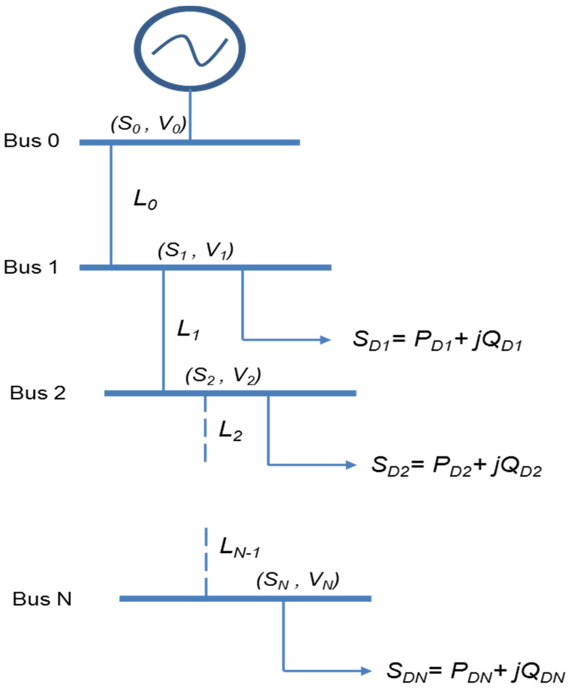
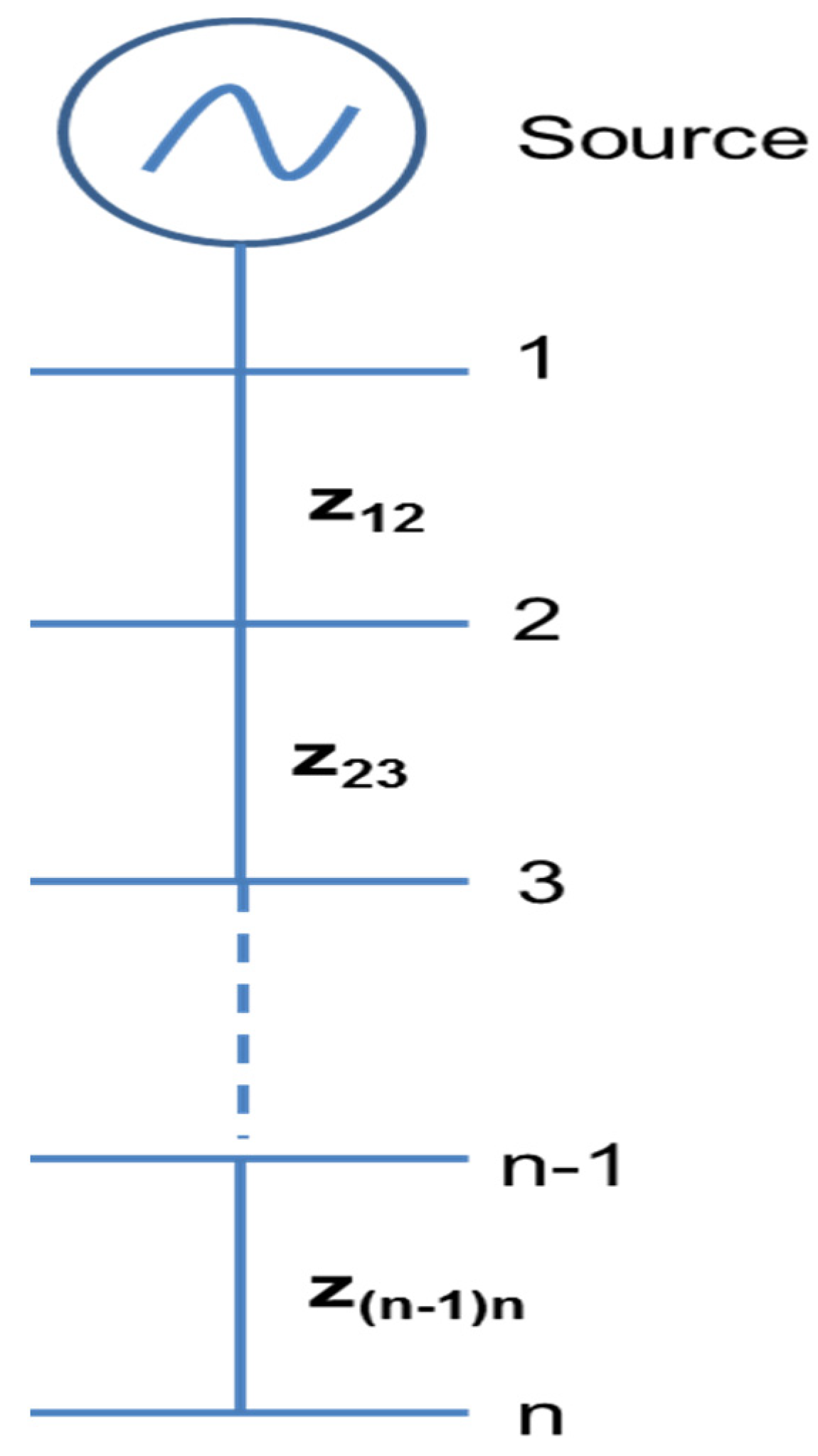
3.1. Analysis of a Distribution Radial Feeder

The single-line diagram in Figure 1 below shows a distribution radial feeder with N buses and N branches. S₀ indicates the apparent power injected by the source at bus 0 with voltage, while V₀ is the source voltage. L₀, L₁, …, and L_N indicate the lines from the source to the bus N, respectively.

Figure 1. Single-line diagram of a distribution feeder with N buses.

The line impedance at each branch and the apparent power at each bus are given by the following general expressions:

$$\begin{gathered} {{\displaystyle z}}_{N-1}={{\displaystyle r}}_{N-1}+j{{\displaystyle x}}_{N-1} \\ {{\displaystyle S}}_{N-1}={{\displaystyle S}}_N+{{\displaystyle S}}_{lossN-1}+{{\displaystyle S}}_{DN-1} \\ {{\displaystyle S}}_N={{\displaystyle S}}_{DN} \end{gathered}$$

(17)

where r and x are the resistance and reactance, S_loss are the losses on each line and S_D is the load apparent power. The voltage at each bus is given by

$${{\displaystyle V}}_{i+1}=\left|{{\displaystyle V}}_i\right|{{\displaystyle \angle \delta }}_i-{{\displaystyle V}}_{zi}$$

(18)

where V_zi is the voltage drop through the impedance Z_i. The power factor (pf₀) at the source is given by

$${{\displaystyle pf}}_0=\frac{{{\displaystyle P}}_0}{{{\displaystyle S}}_0}$$

(19)

It is impractical to find the power factor on each load on a feeder; for analysis purposes, the load power factor is assumed to be the same as the source power factor, i.e.,

$${{\displaystyle pf}}_D={{\displaystyle pf}}_0$$

(20)

The Y_bus of a radial feeder is therefore computed using the diagram below, which is an updated diagram of Figure 2.

Figure 2. The schematic diagram for deriving the Y_bus of a radial feeder.

From Figure 2, the admittances are given by

$$\begin{gathered} y_{12}=\frac{1}{z_{12}} \\ {y}_{23}=\frac{1}{z_{23}} \\ {y}_{\left(n-1\right)n}=\frac{1}{z_{\left(n-1\right)n}} \\ {Y}_{11}=y_{12}; \\ {Y}_{12}=-y_{12}=Y_{21} \\ {Y}_{22}=y_{12}+y_{23}; \\ {Y}_{23}=-y_{23}=Y_{32} \end{gathered}$$

(21)

$$Y_{\left(n-1\right)n}=-y_{\left(n-1\right)n}=Y_{n\left(n-1\right)}$$

(22)

$$Y_{nn}=y_{\left(n-1\right)n}+y_{n\left(n+1\right)}$$

(23)

Since this is a radial feeder, some of the off-diagonal admittances ($Y_{ij}$) are zero. The Y_bus radial feeder with N buses is then found to be

$$Y_{bus}=\left[\begin{array}{ccccc}{Y}_{11}& Y_{21}& 0& \cdots & 0\\ Y_{12}& Y_{22}& Y_{32}& \cdots & 0\\ 0& Y_{23}& \ddots & \cdots & 0\\ 0& 0& \ddots & \ddots & 0\\ \mathrm{⋮}& \mathrm{⋮}& \mathrm{⋮}& Y_{\left(n-1\right)\left(n-1\right)}& Y_{n\left(n-1\right)}\\ 0& 0& 0& Y_{\left(n-1\right)n}& Y_{nn}\end{array}\right]$$

(24)

Therefore, the Y_bus for a radial feeder is applied to the Newton–Raphson Method to obtain the bus voltages and angles as well as the power injections to the buses and line losses.

3.2. The Objective Function and Simulated Annealing Algorithm Applied to a Distribution Feeders

• The objective function: The main objective of optimally placing a distributed generator (DG) on a medium voltage (MV) radial feeder is to ensure that the active and reactive losses are as minimal as possible. In simple terms, the total losses on a radial MV distribution feeder must be minimised when the DG is connected at an optimal position. The minimum and maximum voltages at each bus must not be violated. The thermal ratings of the lines must also not be exceeded. The two conditions mentioned above can be written as follows:

  $${{\displaystyle V}}_{\min }\le {{\displaystyle V}}_{bus}\le {{\displaystyle V}}_{\max }$$

  (25)

In practical situations, the values of the bus minimum and maximum voltages are given as follows:

$$\begin{gathered} {{\displaystyle V}}_{\min }=0.95pu \\ {{\displaystyle V}}_{\max }=1.05pu \end{gathered}$$

(26)

$${{\displaystyle I}}_{line}\le 0.95•{{\displaystyle I}}_{line\_rated}$$

(27)

The objective function is defined as follows:

$$\mathrm{Minimise}f\left(X_i\right)$$

(28)

where $f\left(X_i\right)$ is the total feeder losses, $X_i$ indicates the design point and i the number of iterations subject to the above constraints.

2.

Defining the simulated annealing algorithm:

-

Let f indicates the feeder losses.

-

Choose a value of the starting temperature T, number of predetermined values n = N₋₁ (N = number of buses, n = number of bus, excluding the slack bus) and C, which is the temperature scaling factor.

-

Obtain the base losses f (X₀) using the Newton–Raphson method.

-

Set p = 1 and i = 1.

-

Randomly choose the bus X₁ to connect to the DG too. Compute f (X₁) and

-

∆f = f (X₁) − f (X₀).

-

If ∆f ≤ 0, then accept bus X₁ as the next design point (bus), else if ∆f > 0, then accept X₁ as the next design point with a probability of e^−Δf/kT = e^−Δf/T, since k = 1 for simplicity reasons, else X₁ is rejected. Note the voltage and thermal constraints should not be violated.

-

Set i = i + 1 and repeat steps 4 and 5 above. If i ≥ n, then set p = p + 1, scale the temperature by C and then start in step 3.

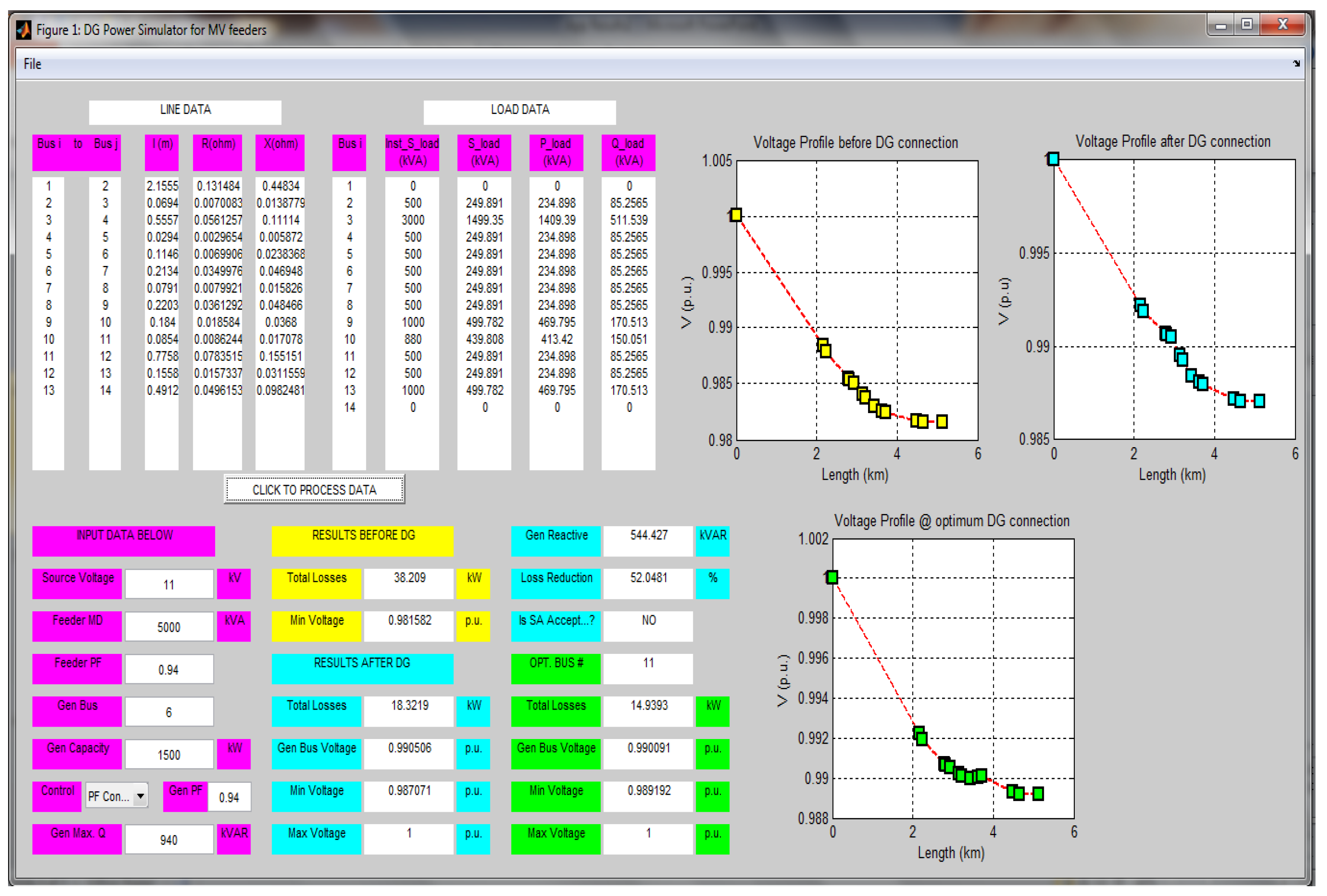
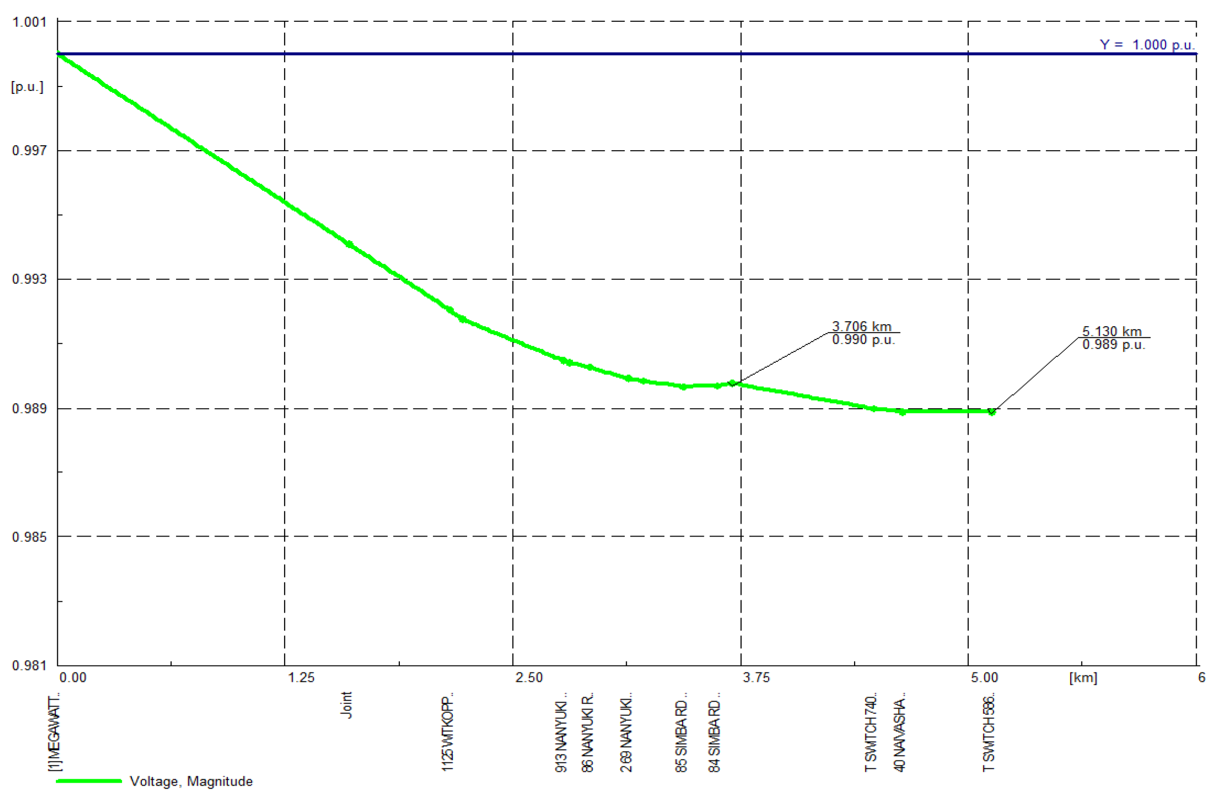
3.3. The Case Study

In this case study, a Megawatt Park-Umngeni 11 kV feeder was used for the demonstration of the application of the simulated annealing algorithm. The feeder feeds from a substation called Megawatt Park. The feeder line data are shown in Table 1.

Table 1. Line data.

Bus i	Bus j	Conductor Type	R1 (ogm/lm)	X1 (ohm/km)	Length (km)	R1 (ohm)	X1 (ohm)
1	2	$11 \mathrm{k}\mathrm{v} 300 \mathrm{m}{\mathrm{m}}^2 Cu PILC 3Core$	0.06100	0.20800	2.15548	0.13148	0.44834
2	3	$11 \mathrm{k}\mathrm{v} 300 \mathrm{m}{\mathrm{m}}^2 Cu PILC 3Core$	0.10100	0.20000	0.06938	0.00701	0.01378
3	4	$11 \mathrm{k}\mathrm{v} 300 \mathrm{m}{\mathrm{m}}^2 Cu PILC 3Core$	0.10100	0.20000	0.55570	0.05613	0.11114
4	5	$11 \mathrm{k}\mathrm{v} 300 \mathrm{m}{\mathrm{m}}^2 Cu PILC 3Core$	0.10100	0.20000	0.02936	0.00297	0.00587
5	6	$11 \mathrm{k}\mathrm{v} 300 \mathrm{m}{\mathrm{m}}^2 Cu PILC 3Core$	0.06100	0.20800	0.11460	0.00699	0.02384
6	7	$11 \mathrm{k}\mathrm{v} 300 \mathrm{m}{\mathrm{m}}^2 Cu PILC 3Core$	1.16400	0.22000	0.21340	0.03500	0.04695
7	8	$11 \mathrm{k}\mathrm{v} 300 \mathrm{m}{\mathrm{m}}^2 Cu PILC 3Core$	0.10100	0.20000	0.07913	0.00800	0.01583
8	9	$11 \mathrm{k}\mathrm{v} 300 \mathrm{m}{\mathrm{m}}^2 Cu PILC 3Core$	0.16400	0.22000	0.22030	0.03613	0.04847
9	10	$11 \mathrm{k}\mathrm{v} 300 \mathrm{m}{\mathrm{m}}^2 Cu PILC 3Core$	0.10100	0.20000	0.18400	0.01858	0.03680
10	11	$11 \mathrm{k}\mathrm{v} 300 \mathrm{m}{\mathrm{m}}^2 Cu PILC 3Core$	0.10100	0.20000	0.08539	0.00862	0.01708
11	12	$11 \mathrm{k}\mathrm{v} 300 \mathrm{m}{\mathrm{m}}^2 Cu PILC 3Core$	0.10100	0.20000	0.77576	0.07835	0.155151
12	13	$11 \mathrm{k}\mathrm{v} 300 \mathrm{m}{\mathrm{m}}^2 Cu PILC 3Core$	0.10100	0.20000	0.15578	0.01573	0.031156
13	14	$11 \mathrm{k}\mathrm{v} 300 \mathrm{m}{\mathrm{m}}^2 Cu PILC 3Core$	0.10100	0.20000	0.49124	0.04962	0.098248

In 2015, the feeder was loaded at a maximum demand (MD) of 5000 kVA and an average power factor of 0.94. The load data of the feeder that corresponds to the MD is shown in Table 2.

Table 2. Load data.

Bus No	SL (kVA)	pf	PL (kW)	QL (kvar)	PL (p.u.)	QL (p.u.)
1	0	0.94	0	0	0	0
2	253	0.94	237.82	86.32	0.04	0.01
3	1518.3	0.94	1427.20	518.01	0.22	0.08
4	253	0.94	237.82	86.32	0.04	0.01
5	253	0.94	237.82	86.32	0.04	0.01
6	253	0.94	237.82	86.32	0.04	0.01
7	253	0.94	237.82	86.32	0.04	0.01
8	253	0.94	237.82	86.32	0.04	0.01
9	506.1	0.94	475.73	172.67	0.07	0.03
10	445.8	0.94	419.05	152.10	0.06	0.02
11	253	0.94	237.82	86.32	0.04	0.01
12	253	0.94	237.82	86.32	0.04	0.01
13	506.1	0.94	475.73	172.67	0.07	0.03
14	0	0.94	0	0	0	0

A load flow study tool that incorporates the Newton–Raphson method was programmed using Matlab (See Figure 3). The Matlab tool is equipped with power factor and constant voltage controls and constant voltage control with reactive power compensation. The graphical user interface of the tool is shown in the figure below. The tool opens a “*.csv” file with feeder information, such as a bus number, conductor impedance and installed capacity at each bus. The data are read and then displayed under “LINE DATA” and “LOAD DATA”.

Figure 3. MATLAB TOOL GUI.

The data that are populated under “LOAD DATA” are the load bus number and the installed capacity at each bus on the feeder. The user, therefore, inputs the feeder’s electrical data such as source voltage, maximum demand (MD), power factor (pf), and the distributed generator’s (DG) proposed bus of connection, capacity, and control (voltage control with reactive power compensation and power factor). The user then presses the “CLICK TO PROCESS DATA” button to run the load flow studies. The results before and after generator connection and during generator connection at an optimal bus are generated. The studies were performed for maximum loading and maximum generation and minimum loading and maximum generation.

The feeder was then modelled in DigSilent Power Factory software, and the simulation was done for three scenarios, namely, (1) before generator connection, (2) with generator connection at a user-defined bus, (3) with generator connection at an optimal bus that was obtained from the Matlab tool. For the generator connection cases, the three control functions for generators were tested. DigSilent Power Factory was used to verify if the Matlab Tool results are precise. The generator used for these studies was a 1500 kW double-fed induction generator (DFIG).

4. Experimental Results

A snapshot of the Matlab tool showing the results of the studies with power factor control and a DG connection 6 is shown in Figure 4. To check the accuracy results, the node voltage values obtained using analytical methods and the exact ones obtained by a load flow computer program are compared. The results show the optimal bus distribution numbers for digital allocation to be bus 6, with the concentrated load method as more accurate.

Figure 4. Matlab tool results with DG connected at bus 6.

The feeder voltage profiles, with DG connected at buses 6 and 11, obtained using DigSilent Power Factory are shown in Figure 5 and Figure 6. The blue curve is the voltage profile without DG. The yellow curve correspond to the voltage profile with DG operating at different power factors. It appears that the maximum power that can be generated by the DG without violating voltage limits decreases piecewise linearly with distance from the substation.

Figure 5. Voltage profile with DG connected at bus 6.

Figure 6. Voltage profile with DG connected at bus 11.

The summary of the results including all the other scenarios that were considered is shown in Table 3 and Table 4.

Table 3. Summary of results with MD = 5000 kVA.

Bus for DG Connection	DG Control Function	Description of Feeder Results	Simulation Results with Matlab Tool	Simulation Results with DigSilent Power Factory	% Error
Not applicable (Before DG connection)	Not applicable	Losses (kW)	38.21	38.57	0.93
		Minimum Voltage (p.u.)	0.98158	0.98172	0.01
Bus 6	Power Factor Control	Losses (kW)	18.32	18.68	1.93
		Generator Bus Voltage (p.u.)	0.99051	0.99047	0.00
		Minimum Voltage (p.u.)	0.98707	0.98708	0.00
		Loss Reduction (%)	52.05	51.57	0.93
	Constant Voltage Control	Losses (kW)	17.25	17.74	2.76
		Generator Bus Voltage (p.u.)	0.99250	0.99236	0.01
		Minimum Voltage (p.u.)	0.98908	0.98897	0.01
		Loss Reduction (%)	54.85	54.01	1.55
	Constant Voltage Control with reactive power compensation	Losses (kW)	18.06	18.9	4.44
		Generator Bus Voltage (p.u.)	1.00000	1.00000	0.00
		Minimum Voltage (p.u.)	0.99660	0.99658	0.00
		Reactive compensation (kVar)	1500	1600	6.25
		Difference in Q-compensations (kVar)	100
		Loss Reduction (%)	52.73	51.00	3.29
Bus 14 (End of feeder)	Power Factor Control	Losses (kW)	16.24	16.66	2.52
		Generator Bus Voltage (p.u.)	0.99226	0.99207	0.02
		Minimum Voltage (p.u.)	0.98996	0.98965	0.03
		Loss Reduction (%)	57.50	56.81	1.20
	Constant Voltage Control	Losses (kW)	15.78	16.29	3.13
		Generator Bus Voltage (p.u.)	0.99572	0.99546	0.03
		Minimum Voltage (p.u.)	0.99231	0.99212	0.02
		Loss Reduction (%)	58.70	57.77	1.60
	Constant Voltage Control with reactive power compensation	Losses (kW)	16.88	17.58	3.98
		Generator Bus Voltage (p.u.)	1.00000	1.00000	0.00
		Minimum Voltage (p.u.)	0.99493	0.99490	0.00
		Reactive compensation (kVar)	494	600	17.67
		Difference in Q-compensations (kVar)	106
		Loss Reduction (%)	55.82	54.42	2.51
Bus 11 (Optimal Bus)	Power Factor Control	Losses (kW)	14.94	15.35	2.67
		Generator Bus Voltage (p.u.)	0.99009	0.99004	0.01
		Minimum Voltage (p.u.)	0.98919	0.98888	0.03
		Loss Reduction (%)	60.90	60.20	1.15
	Constant Voltage Control	Losses (kW)	13.94	14.49	3.80
		Generator Bus Voltage (p.u.)	0.99263	0.99243	0.02
		Minimum Voltage (p.u.)	0.99173	0.99156	0.02
		Loss Reduction (%)	63.52	62.43	1.71
	Constant Voltage Control with reactive power compensation	Losses (kW)	15.69	16.59	5.42
		Generator Bus Voltage (p.u.)	1.00000	1.00000	0.00
		Minimum Voltage (p.u.)	0.99789	0.99788	0.00
		Reactive compensation (kVar)	1159	1200	3.42
		Difference in Q-compensations (kVar)	41
		Loss Reduction (%)	58.94	56.99	3.31

Table 4. Summary of Results with MD = 3000 kVA.

Bus for DG Connection	DG Control Scheme	Description of Result	Simulation Results with Matlab Tool @ MD = 5 MVA	Simulation Results with Matlab Tool @ MD = 3 MVA
Not applicable Before DG connection)	Not applicable	Losses (kW)	38.21	13.81
		Minimum Voltage (p.u.)	0.98158	0.98898
Bus 6	Power Factor Control	Losses (kW)	18.32	3.72
		Generator Bus Voltage (p.u.)	0.99051	0.99641
		Minimum Voltage (p.u.)	0.98707	0.99435
		Loss Reduction (%)	52.05	73.06
		Optimal Bus Number	11	10
Bus 6	Constant Voltage Control	Losses (kW)	17.25	3.5
		Generator Bus Voltage (p.u.)	0.9925	0.99839
		Minimum Voltage (p.u.)	0.98908	0.99633
		Loss Reduction (%)	54.85	74.66
		Optimal Bus Number	11	9
Bus 6	Constant Voltage Control with reactive power compensation	Losses (kW)	18.06	3.72
		Generator Bus Voltage (p.u.)	1	1
		Minimum Voltage (p.u.)	0.99660	0.99795
		Loss Reduction (%)	52.73	95.02
		Optimal Bus Number	11	10
		ReactivePower Compensation	1500	324
Bus 10 (Optimal Bus when using PF Control)	Power Factor Control	Losses (kW)		2.58
		Generator Bus Voltage (p.u.)		0.99685
		Minimum Voltage (p.u.)		0.99624
		Loss Reduction (%)		81.32

The siting of DGs at various locations shows a positive impact on voltage profiles. However, there is a possibility of voltage rise if the DG penetration level is too high. The rise in voltage could cause misoperation of protective devices, and therefore adjustment or changes of protective devices are required. In order to accommodate more DGs, the voltage profile along the feeder should be kept within statutory limits (voltage between ± 10% of the base voltage), and there is a need to employ intelligent devices for this purpose. The development of the smart grid allows for the use of intelligent devices and thus helps to keep the voltage level within statutory limits.

5. Discussion of Results

The Matlab tool is intended to be utilised by network planning engineers when responding to independent power producers (IPPs) inquiries for generator connection on a medium voltage distribution radial feeder. Due to the number of inquiries that might be received in a day and the amount of work that is handled by network planning engineers, the time to do proper network load flow studies, using power simulation packages, for each inquiry received might be very limited. The tool will therefore ensure that a network planning engineer can do a quick power system analysis study and be able to give feedback to an IPP or customer within a reasonable time.

Depending on where the IPP is proposing to connect their generator on the feeder, the network planning engineer can therefore advise on the optimal point of connection on the feeder, and this can also assist the customer to obtain a servitude for building their power plants closest to the optimal point of the connection while at the very same time assisting the electrical utility company in reducing the losses on the feeder.

From the results obtained using the Matlab tool, it is clear that before connecting a distributed generator the voltage drops exponentially according to the feeder distance from the source. From the studies that were performed, the losses were reduced by 52% and the minimum voltage of the feeder was improved from 99.16% to 98.71% (on power factor control), 99.91% (on constant voltage control) and 99.66% (on constant voltage control with reactive power compensation) when the distributed generator was connected to bus 6, which is the bus assumed to be where an independent power producer planned to connect their generator.

From the voltage profiles, the bus voltages at the generator’s connection bus also showed improvement. The generator reactive power that could be achieved on power factor control with a power factor of 0.94 was 544 kVAR, and this led to a generator bus voltage of 99.05%. For voltage control, the generator pumped more VARs into the network to try and regulate the voltage to 1 p.u, but the generator reactive power was limited to the maximum reactive power of 940 kVAR, which was not enough to regulate the voltage to 1 p.u. The generator bus voltage obtained from the injection of 940 kVAR was 99.25%.

For the constant voltage control scheme with reactive power compensation, the voltage improved up to 1 p.u. When connecting a distributed generator at the end of the feeder, bus 14 in this case, the feeder losses were reduced by about 57.5% and 55.8% and the minimum voltages of the feeder were improved from 99.16% to 99.996% and 99.493% on constant power factor control and constant voltage control with reactive power compensation, respectively.

The main aim of the whole study was to find an optimal point where a distributed generator can be connected to a medium voltage radial feeder. The Matlab tool created to perform the instruction of finding the optimal bus chose bus 11 as the optimum bus. The results obtained from connecting the distributed generator to bus 11 showed that the loss reduction was about 60% and the feeder minimum voltages were found to be 98.99% and 99.79% on power factor control and constant voltage control with reactive power compensation, respectively.

Minimum voltage results obtained from applying power factor and voltage control schemes indicated that the end of the feeder is the point of connection when voltage improvement is the key element to be achieved. Connecting a 1.5 MW distributed generator anywhere on a radial feeder except for the busbar at the substation will result in reduced losses and improved feeder minimum voltage on the radial feeder.

The results obtained from using DigSilent PowerFactory presented similar behaviours as those obtained from the Matlab Tool. The thermal loading of the feeder was not computed in the Matlab Tool because it is known that the feeder is not thermally constrained; however, the thermal loading was noted when performing the load flow studies using DigSilent PowerFactory. For the base case, i.e., before connecting the generator, the section of the feeder with the highest thermal loading was found to be the one closest to the source. When connecting a distributed generator to the feeder, the thermal loading of the section of the feeder closest was reduced according to the size of the generator.

The losses obtained from the two tools had maximum errors of 2.67%, 3.8% and 5.42% with a distributed generator operating under power factor control, constant voltage control and constant voltage control with reactive power compensation, respectively. It was also observed that the losses obtained from using DigSilent PowerFactory were always higher than those obtained from using the Matlab Tool.

The bus voltages had an error of less than 1%. For the constant voltage control with reactive power compensation on the PowerFactory simulation, it was observed that the reactive power compensation value required to achieve a bus-controlled voltage of 1 per unit was always about 40–100 kVAR higher than the one obtained from the Matlab Tool. This might be since the DFIG template that was used when simulating consists of a 0.4/11 kV step-up transformer, which absorbs about 100 kVAR; the Matlab Tool assumed that the generator is connected directly to the 11 kV network without the need to use the step-up transformer. It was observed that the value of reactive power compensation that was required to achieve a voltage of 1 p.u. at a point connection dropped as the connection point moved away from the source.

Connecting a generator at bus 11 will result in a saving of 38.21 − 14.94 = 23.27 kW. An RDP (Reconstruction and Development Programme) house in South Africa has a notified maximum demand (NMD) of about 2.5 kW. The number of RDP houses that can be supplied from the saved losses is 9. If each kilowatt-hour of electricity costs R1.35, then the total cost that can be recovered from the losses is about 1.35 * 9 * 24 = R291.60 per day, which translates to R106 434 per annum assuming that the generator is running for 24 h per day. The more generators are optimally connected on more than one radial feeder, the more losses can be reduced on the medium voltage network and the more houses without power can be electrified.

The Matlab Tool was also used to perform studies when the feeder load was considered to be light, i.e., 60% of the maximum demand of 5000 kVA = 3000 kVA, with an assumption that the results obtained would be very similar to when simulating with DigSilent PowerFactory. The tool indicated that bus 10 was the optimal bus for connecting a distributed generator when using power factor control. In this case, the losses before connecting the generator were sitting at 13.8 kW, and after connecting the generator at the optimal bus, the losses were reduced to 2.58 kW with a feeder minimum voltage of 99.62%. The generator bus voltage was sitting at 99.685%. When comparing the results of the heavy-loaded feeder and light-loaded feeder, it is clear that when a load of a feeder is light, then the bus voltages will rise.

Environmentally, this Matlab tool will not have any environmental impacts and it will not put the public in any danger. However, it should be stressed that renewable energy generators such as wind farms and solar and tidal waves do have an impact on the environment. As discussed in the introduction, they can cause traffic during their construction, noise when they are operating and air pollution during their manufacturing.

Simulated annealing optimisation was used because it relates well to the problem at hand. The coding of the optimisation method in Matlab was not complex, but setting up the code to the point where the optimisation could be coded was a bit of a challenge, especially for one not familiar with the Matlab programming language. The limitation with this optimisation method is that it cannot tell that it has found the optimal point, and one used additional functionality to determine the exact optimal point. Another disadvantage is that there os a trade-off between the quality of the result and the time taken for the algorithm to run.

6. Remarks and Conclusions

The objective of the study was to investigate the optimal placement of a distributed generator on a medium voltage radial feeder. Simulated annealing optimisation was used to find an optimal bus for connecting a distributed generator to a radial feeder.

A Matlab tool for performing load flow studies on medium voltage radial feeders with distributed generation was developed. The tool incorporates a simulated annealing optimisation algorithm to identify an optimal bus for distributed generator connection.

For a radial feeder, the voltage drops according to the distance from the source, i.e., the further away from the source, the more voltage drops on the feeder. The section of the feeder that carries most of the load was the one closest to the source. We have also shown that a connection of a 1.5 MW distributed generator anywhere, except the source busbar, on a radial feeder loaded at 5 MVA results in reduced losses, and connecting a distributed generator at an optimal position results in maximum loss reduction.

The optimal point of connecting a distributed generator depends on the loading of the feeder and the control function of the distributed generator. A distributed generator operating on a feeder with reduced load demand leads to a voltage rise. The generation might need to be reduced to ensure that maximum voltage constraints are not violated. Furthermore, the results showed less reactive power compensation as required when the generator connection moves away from the source.

The Matlab tool created in this research can be used to perform load flow studies in cases where the time available is very limited, provided the feeder information such as conductor type, section length and installed capacity is available and well tabulated in excel.

The study has shown how DigSilent PowerFactory can be used to perform load flow studies on medium voltage radial feeders with distributed generators. Future work will include investigating a feeder with multiple branches, taking into consideration fault levels when connecting a distributed generator and also ensuring that the basics of optimisation mathematics are covered to avoid delays, and further optimise the Matlab program for easy troubleshooting.

References

1. Manzamo-Agugliaro, F.; Alcayde, A.; Montoya, F.G. Scientific production of renewable energies worldwide: An overview. Renew. Sustain. Energy Rev. 2013, 18, 134–143. [Google Scholar] [CrossRef]
2. Fossil Fuel. Available online: http://www.sciencedaily.com/articles/f/fossil_fuel.htm (accessed on 20 April 2022).
3. Fossil Fuel. Available online: http://en.wikipedia.org/wiki/Fossil_fuel (accessed on 20 April 2022).
4. Impact of Fossil Fuel. Available online: http://geoscience.wisc.edu/~chuck/Geo106/lect24.html (accessed on 20 April 2022).
5. Pazheri, F.R.; Al-Arainy, A.A.; Othman, M.F.; Malik, N.H. Global renewable electricity potential. In Proceedings of the GCC Conference and Exhibition (GCC), Doha, Qatar, 17–20 November 2013; pp. 59–63. [Google Scholar]
6. Williams, A. Role of fossil fuels in electricity generation and their environmental impact. IEE Proc. A Sci. Meas. Technol. 1993, 140, 8–12. [Google Scholar] [CrossRef]
7. Turner, W.; Western, J. Nuclear energy’s role in a more sustainable future. In Proceedings of the Opportunities and Advances in International Electric Power Generation, International Conference, Orlando, FL, USA, 18–20 March 1996; Volume 1, pp. 81–86. [Google Scholar]
8. Rashad, S.M. Nuclear Power and the Environment Prospects and Challenges. In Proceedings of the Radio Science Conference, Proceedings of the Twenty Third National, Menouf, Egypt, 14–16 March 2006; pp. 1–32. [Google Scholar]
9. Available online: http://www.empr.gov.bc.ca/EAED/AEPB/Documents/CleanEnergyJune.pdf (accessed on 20 April 2022).
10. Mohibullah, M.; Radzi, A.M.; Hakim, M.I.A. Basic design aspects of micro hydro power plant and its potential development in Malaysia. In Proceedings of the Power and Energy Conference Proceedings, Kuala Lumpur, Malaysia, 29–30 November 2004; pp. 220–223. [Google Scholar]
11. Sriram, N.; Shahidehpour, M. Renewable biomass energy. In Proceedings of the Power Engineering Society General Meeting, San Francisco, CA, USA, 12–16 June 2005; Volume 1, pp. 612–617. [Google Scholar]
12. Kellas, A. Biomass and electrical energy. In Proceedings of the 7th Mediterranean Conference and Exhibition on Power Generation, Transmission, Distribution and Energy Conversion, Ayia Napa, Cyprus, 7–10 November 2010; pp. 1–7. [Google Scholar]
13. Biomess Energy. Available online: http://www.northblythproject.co.uk/biomass-energy/ (accessed on 25 March 2022).
14. Renewable Energy. Available online: http://www.window.state.tx.us/specialrpt/energy/renewable/ (accessed on 25 March 2022).
15. Solar Systems. Available online: www.kids.esdb.bg/solar.html (accessed on 24 April 2022).
16. Solar Power Systems. Available online: http://en.wikipedia.org/wiki/Concentrated_solar_power (accessed on 30 March 2022).
17. Freris, L.; Infield, D. Renewable Energy in Power Systems; John Wiley and Sons: Hoboken, NJ, USA, 2020. [Google Scholar]
18. PowerFactory Training Notes. Introduction to Renewable Energy Generation; DigSilent Buyisa: Centurion, South Africa, 2019. [Google Scholar]
19. Available online: http://www.irena.org (accessed on 30 March 2022).
20. Siraj, K.; Siraj, H.; Nasir, M. Modeling and control of a doubly fed induction generator for grid integrated wind turbine. In Proceedings of the 2022 16th International Power Electronics and Motion Control Conference and Exposition (PEMC), Antalya, Turkey, 21–24 September 2014; pp. 901–906. [Google Scholar]
21. Available online: http://en.wikipedia.org/wiki/Photovoltaic_power_station (accessed on 3 April 2022).
22. Available online: www.eskom.co.za (accessed on 30 March 2022).
23. Sharma, V.V.; Chawla, H. Integrated renewable systems. In Proceedings of the Power, Control and Embedded Systems (ICPCES), 2nd International Conference, Allahabad, India, 17–19 December 2012; pp. 1–6. [Google Scholar]
24. Wind Turbine Foundations. Available online: http://wind-turbine.tripod.com (accessed on 15 March 2022).
25. Energy Systems. Available online: http://www.esru.strath.ac.uk (accessed on 20 March 2022).
26. Matlab. Available online: www.mathworks.com (accessed on 25 March 2022).
27. Department of Mineral Resources and Energy. Available online: www.energy.gov.za (accessed on 15 March 2022).
28. South African Weather Services. Available online: www.weathersa.co.za (accessed on 15 March 2022).
29. Renewable Energy World. Available online: http://www.renewableenergyworld.com (accessed on 27 April 2022).
30. Global Warming 101. Available online: www.nrdc.org/globalwarming/ (accessed on 27 January 2022).
31. Radioactive Waster. Available online: http://en.wikipedia.org/wiki/Radioactive_waste (accessed on 15 March 2022).
32. Hydropower Industry. Available online: http://www.internationalrivers.org/environmental-impacts-of-dams (accessed on 17 March 2022).
33. Available online: http://www.oregon.gov/ODOT/HWY/OIPP/docs/ (accessed on 17 March 2022).
34. Khani, D.; Yazdankhah, A.S.; Kojabadi, H.M. Impacts of distributed generations on power system transient and voltage stability. Int. J. Electr. Power Energy Syst. 2012, 43, 488–500. [Google Scholar] [CrossRef]
35. Rao, S.S. Engineering Optimization: Theory and Practice, 4th ed.; Wiley: Hoboken, NJ, USA, 2009. [Google Scholar]
36. Walsh, G.R. Methods of Optimization, 1st ed.; John Wiley and Sons: Hoboken, NJ, USA, 1975. [Google Scholar]
37. Nemhauser, G.L.; Rinnooy, K.A.H.G.; Todd, M.J. Optimization, Handbooks in Operations Research and Management Science; Elsevier Science: North-Holland, The Netherlands, 1989; Volume 1. [Google Scholar]
38. Raghavjee, R.; Pillay, N. A Comparison of Genetic Algorithms and Genetic Programming in Solving the School Timetabling Problem. In Proceedings of the Fourth World Congress on Nature and Biologically Inspired Computing (NaBIC), Mexico City, Mexico, 5–9 November 2012; pp. 98–103. [Google Scholar]
39. Sickel, K.; Hornegger, J. Genetic Programming for Expert Systems. In Proceedings of the IEEE Congress on Evolutionary Computation, Barcelona, Spain, 18–23 July 2010; pp. 1–8. [Google Scholar]
40. Filho, J.L.R.; Treleaven, P.C.; Alippi, C. Genetic-algorithm programming environments. Computer 1994, 27, 28–43. [Google Scholar] [CrossRef]
41. del Valle, Y.; Venayagamoorthy, G.K.; Mohagheghi, S.; Hernandez, J.C.; Harley, R.G. Particle Swarm Optimization: Basic Concepts, Variants and Applications in Power Systems. IEEE Trans. Evol. Comput. 2008, 12, 171–195. [Google Scholar] [CrossRef]
42. Dorigo, M.; Birattari, M.; Stutzle, T. Ant colony optimization. IEEE Comput. Intell. Mag. 2006, 1, 28–39. [Google Scholar] [CrossRef]
43. Alkandari, A.M.; Soliman, S.A.; Mantwy, A.H. Simulated annealing optimization algorithm for electric power systems quality analysis: Harmonics and voltage flickers. In Proceedings of the 2008 12th International Middle East Power System Conference—MEPCON, Aswan, Egypt, 12–15 March 2008; pp. 287–293. [Google Scholar]
44. Li, Y.; Czarkowski, D.; de Leon, F. Optimal Distributed Voltage Regulation for Secondary Networks with DGs. IEEE Trans. Smart Grid 2012, 3, 959–967. [Google Scholar]
45. Lee, S.H.; Park, J. Optimal Placement and Sizing of Multiple DGs in a Practical Distribution System by Considering Power Loss. IEEE Trans. Ind. Appl. 2013, 49, 2262–2270. [Google Scholar] [CrossRef]
46. Foster, J.; Berry, A.M.; Boland, N.; Waterer, H. Comparison of Mixed-Integer Programming and Genetic Algorithm Methods for Distributed Generation Planning. IEEE Trans. Power Syst. 2022, 29, 833–843. [Google Scholar] [CrossRef]
47. Duong, Q.H.; Mithulananthan, N. Multiple Distributed Generator Placement in Primary Distribution Networks for Loss Reduction. IEEE Trans. Ind. Electron. 2013, 60, 1700–1708. [Google Scholar]
48. Kashem, M.A.; Ganapathy, V.; Jasmon, G.B.; Buhari, M.I. A novel method for loss minimization in distribution networks. In Proceedings of the International Conference on Electric Utility Deregulation and Restructuring and Power Technologies, London, UK, 4–7 April 2000; pp. 251–256. [Google Scholar]
49. George, S.P.; Ashok, S.; Bandyopadhyay, M.N. Impact of distributed generation on protective relays. In Proceedings of the 2013 International Conference on Renewable Energy and Sustainable Energy (ICRESE), Coimbatore, India, 5–6 December 2013; pp. 157–161. [Google Scholar]
50. National Energy Regulator of South Africa. Grid Connection Code for Renewable Power Plants (RPPs) Connected to the Electricity Transmission System (TS) or Distribution System (DS) in South Africa; National Energy Regulator of South Africa: Pretoria, South Africa, 2022.
51. Azmy, A.M.; Erlich, I. Impact of distributed generation on the stability of electrical power system. In Proceedings of the IEEE Power Engineering Society General Meeting, San Francisco, CA, USA, 12–16 June 2005; Volume 2, pp. 1056–1063. [Google Scholar]
52. Slootweg, J.G.; Kling, W.L. Impacts of distributed generation on power system transient stability. In Proceedings of the Power Engineering Society Summer Meeting, Chicago, IL, USA, 21–25 July 2002; Volume 2, pp. 862–867. [Google Scholar]
53. Camilo, L.; Cebrian, J.C.; Kagan, N.; Matsuo, N.M. Impact of distributed generation units on the sensitivity of customers to voltage sags. In Proceedings of the 8th International Conference and Exhibition on Electricity Distribution (CIRED 2005), Turin, Italy, 6–9 June 2005; pp. 1–4. [Google Scholar]
54. Caples, D.; Boljevic, S.; Conlon, M.F. Impact of distributed generation on voltage profile in 38kV distribution system. In Proceedings of the 2011 8th International Conference on the European Energy Market (EEM), Zagreb, Croatia, 25–27 May 2011; pp. 532–536. [Google Scholar]