
Multi-Fractional Brownian Motion: Estimating the Hurst Exponent via Variational Smoothing with Applications in Finance


Abstract
:1. Introduction
Contributions
2. Definitions and Main Properties
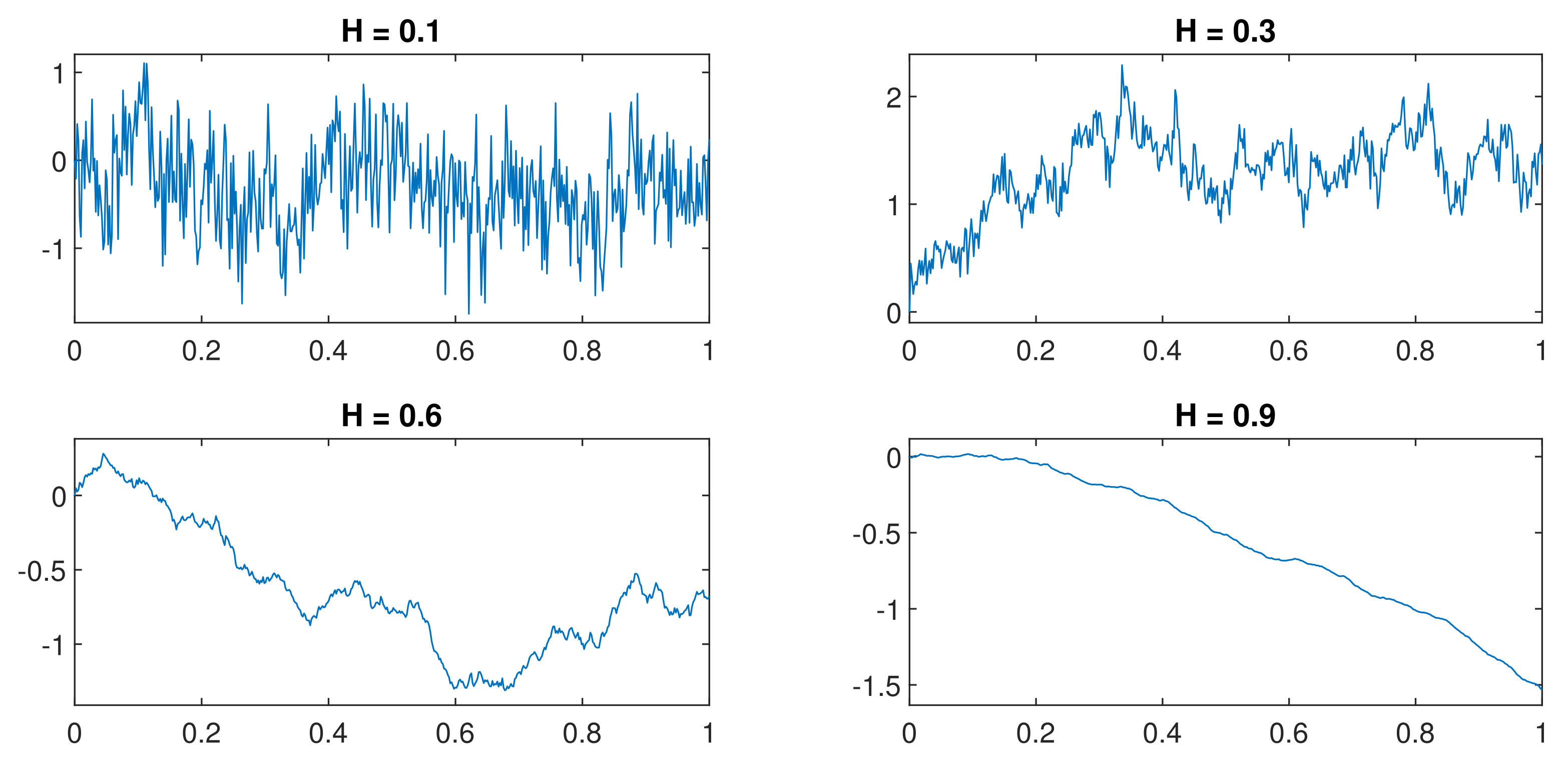
2.1. fBm
- .
- It is a Gaussian process with .
- It has a covariance function
- if , then is the classical Brownian motion.
- if , the increments of are negatively correlated and the process exhibits short-range dependence, i.e., it is more likely that the trend is broken.
- if , the increments of are positively correlated and the process exhibits long-range dependence, i.e., it is more likely that the trend is preserved.
- If , the dependence decays exponentially and , so the increments have opposite signs, and the particle (or price, etc.) tends to return, denoting a mean reversion. Such a process is called anti-persistent and is said to exhibit short-range dependence.
- If , the dependence decays slower than exponential and , so the particle tends to insist on the same direction. Such a process is called persistent and is said to exhibit long-range dependence.
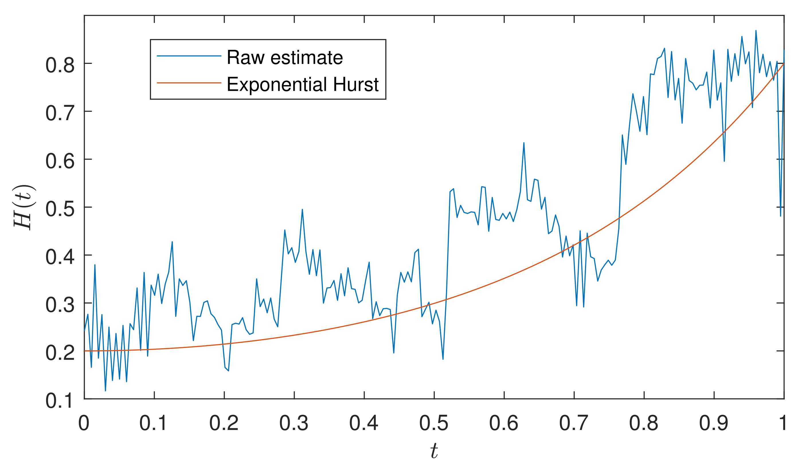
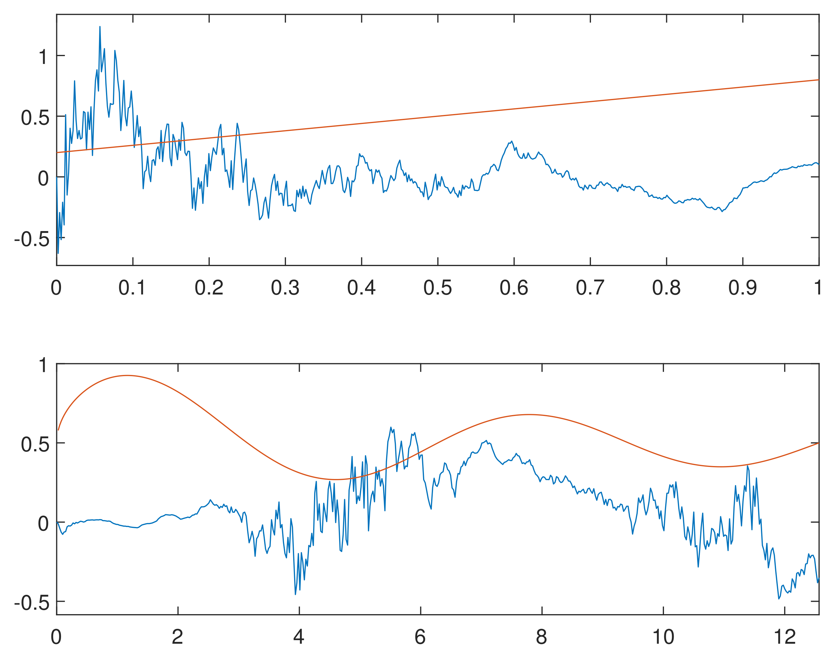
2.2. mBm
3. Simulation of Sample Paths
- Compute the eigenvalues of C with the fast Fourier transform (FFT) of its first row.
- Compute as a complex standard normal random vector: generate , while for , generate two independent ; then compute
- A sample of fGn is obtained by computing the FFT of
- A sample of fBm at times k is given by the cumulative sum of X. Thanks to the self-similarity of fBm, the rescaled fBm on an interval partitioned in points with distance , is obtained by multiplying the cumulative sum of X by . Finally, we have to set the first value to 0, since fBm is a process starting at 0.
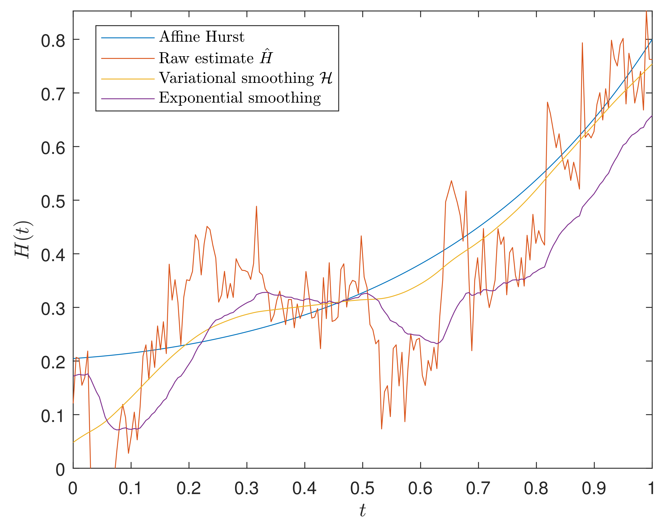
4. Estimation of the Hurst Exponent
Smoothing
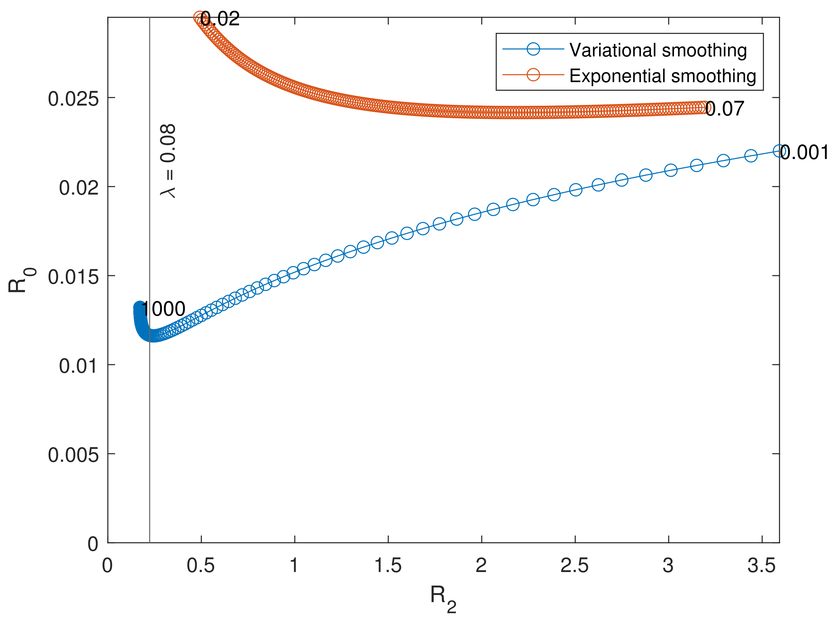
5. Accuracy Test
- The mean integrated squared error, representing the average accuracy of the method:
- The average bias at , representing the ability of the technique not to create artificial gaps at the border:
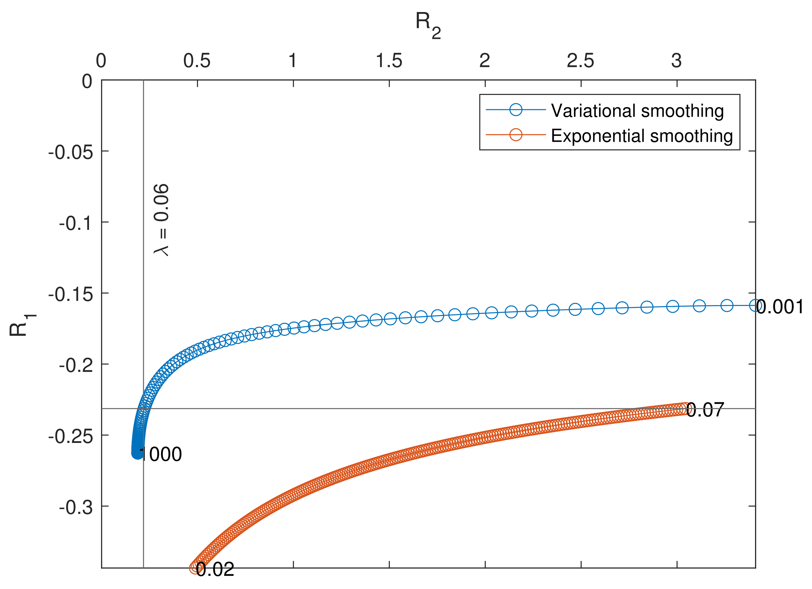
- The average quadratic slope, determining to which extent the erratic estimate has been smoothed:
- Generate 100 mBm trajectories and compute the associated raw estimates.
- Define a set of 200 logarithmically spaced (the variational smoothing method is sensitive to small values of ) parameters between decades and , and a set of 200 evenly spaced parameters between 0.02 and 0.07. Compute the smooth estimates of the raw ones from the previous step.
- For each smooth estimate, compute the three accuracy metrics.
- For each parameter, compute the average metrics and visualize the results with plots: R2 vs. R0 and R2 vs. R1.
6. Simulation of Financial Data
- Compute the smooth version of the raw estimate .
- Forecast by means of a second-order Taylor expansion. Consider a smooth function f on an equispaced grid with step , and approximate the first derivative with the first order backward difference and the second derivative with the second order backward difference:Hence, applying the same rule for the smooth Hurst exponents, we obtain
- Estimate the scale parameter by Equations (5) and (6) in the case of the absolute moment of order 1 and solving forThe raw estimation and its smoothing are distinct steps of the estimation procedure, but it is reasonable to assume that the time steps in both computations are the same. Therefore, we can write the estimate of the scale parameter as
- Estimate the underlying standard Bm W that appears in the definition of the mBm (2). Firstly, notice that in this case , so the first integral in the definition vanishes. Moreover, since at the origin t of the time interval the mBm has to be 0, we translate X by , obtainingThe integral on the rhs, call it I, can be approximated using the Riemann sum asMoving the first on the other side and definingwe can writeNow, since equals 1 when , we can move the term out from the series, obtaining
- Recall that X is a log price, i.e., , where P is the price of the financial asset; thus, its increment can be written aswhere r is known as log return. We will exploit this relation to compute the forecasted log price . However, first, we have to derive the formula for the log return. Consider the increment of the mBm at time , then add and subtract and rearrange the terms in order to reach a form resembling the left-hand side of Equation (7) (with the term moved to the right-hand side)Applying (7) to the two terms and combining the two series, we arrive at the formula for the log price
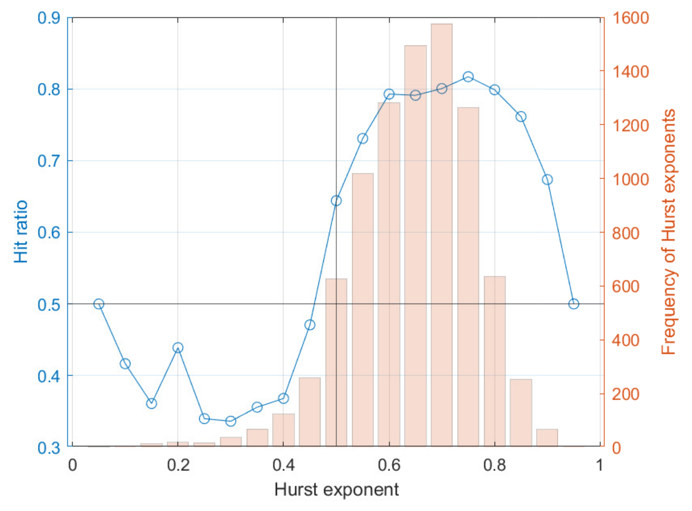
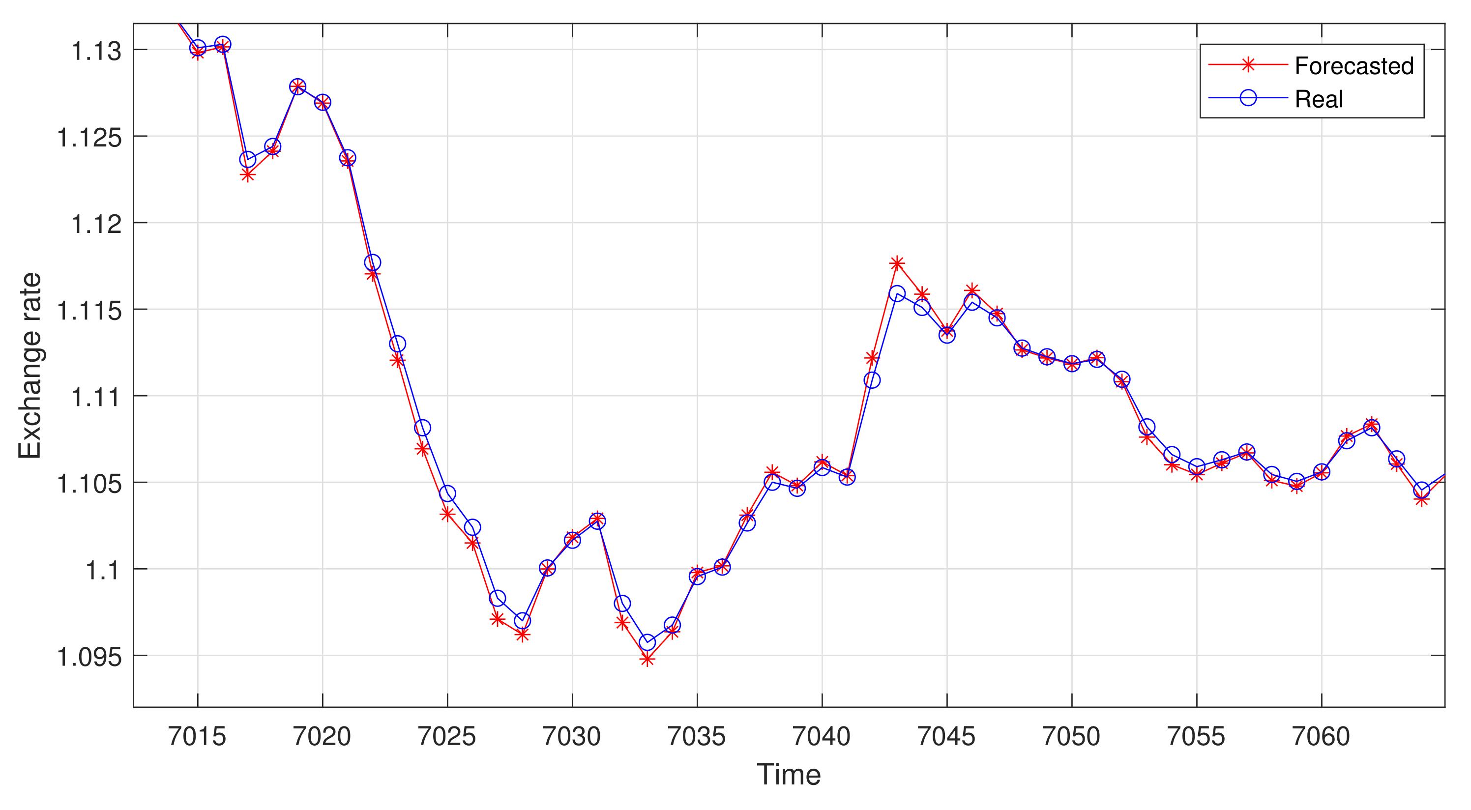
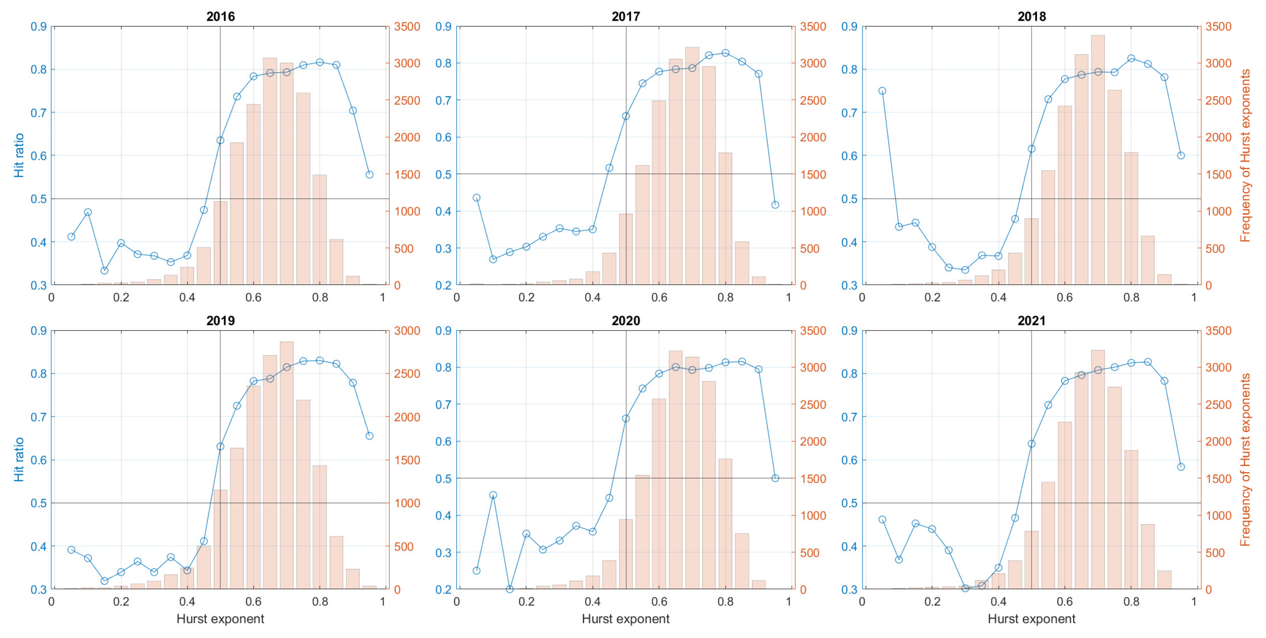
6.1. One-Step Forecasting
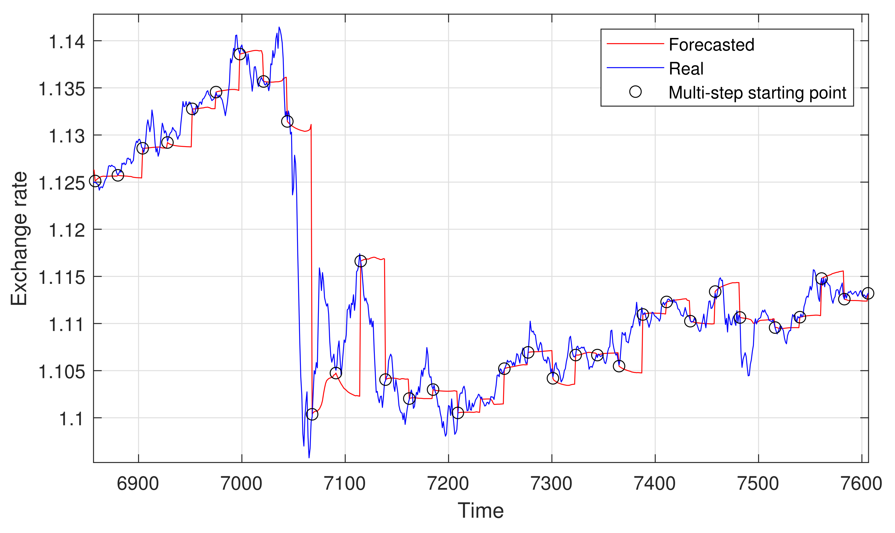
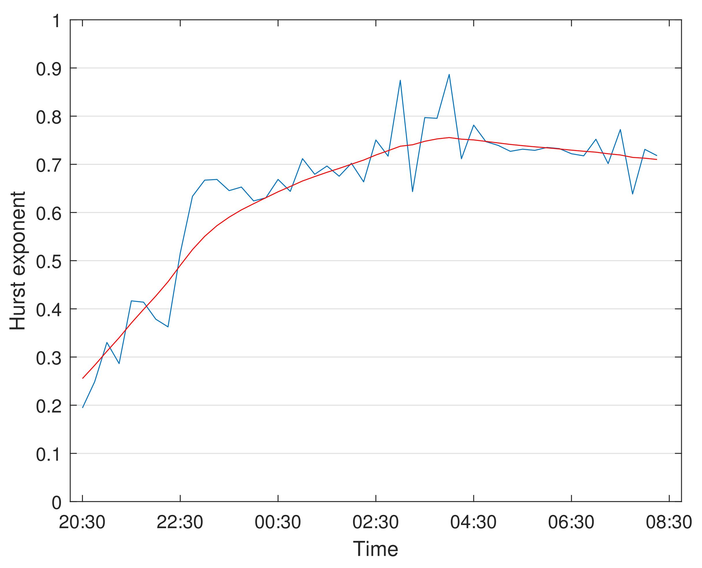
6.2. Multi-Step Forecasting
- The fast variation of H in time (as seen in Figure 7), which seems to be hard to catch with this approach.
- A flaw inherent in the very nature of the multi-stage prediction: the propagation of errors. This approach uses past predicted values to compute new ones, so previous errors are propagated into future predictions.
7. Conclusions
Author Contributions
Funding
Institutional Review Board Statement
Informed Consent Statement
Data Availability Statement
Acknowledgments
Conflicts of Interest
References
- Cont, R. Empirical properties of asset returns: Stylized facts and statistical issues. Quant. Financ. 2001, 1, 223–236. [Google Scholar] [CrossRef]
- Bianchi, S. Pathwise identification of the memory function of multifractional Brownian motion with application to finance. Int. J. Theor. Appl. Financ. 2005, 8, 255–281. [Google Scholar] [CrossRef]
- Biagini, F.; Sulem, A.; Øksendal, B.; Wallner, N.N. An introduction to white-noise theory and Malliavin calculus for fractional Brownian motion. Proc. R. Soc. 2004, 460, 347–372. [Google Scholar] [CrossRef]
- Rogers, L.C.G. Arbitrage with fractional Brownian motion. Math. Financ. 1997, 7, 95–105. [Google Scholar] [CrossRef] [Green Version]
- Cheridito, P. Arbitrage in fractional Brownian motion models. Financ. Stoch. 2003, 7, 533–553. [Google Scholar] [CrossRef]
- Staszkiewicz, P.; Łosiewicz-Dniestrzańska, E.; Grygiel-Tomaszewska, A. European financial institution physical geolocation and the high-frequency trading potential. In The Digitalization of Financial Markets; Marszk, A., Lechman, E., Eds.; Routledge: London, UK, 2021; pp. 19–37. [Google Scholar]
- Bezborodov, V.; Di Persio, L.; Mishura, Y. Option Pricing with Fractional Stochastic Volatility and Discontinuous Payoff Function of Polynomial Growth. Methodol. Comput. Appl. Probab. 2019, 21, 331–366. [Google Scholar] [CrossRef] [Green Version]
- Alvarez-Ramirez, J.; Alvarez, J.; Rodriguez, E.; Fernandez-Anaya, G. Time-Varying Hurst Exponent for US Stock Markets. Phys. A 2008, 387, 6159–6169. [Google Scholar] [CrossRef]
- Jiang, J.; Ma, K.; Cai, X. Non-linear characteristics and long-range correlations in Asian stock markets. Phys. A 2007, 378, 399–407. [Google Scholar] [CrossRef]
- Bianchi, S.; Pianese, A. Multifractional Processes in Finance. SSRN Electron. J. 2014, 5, 1–22. [Google Scholar] [CrossRef]
- Corlay, S.; Lebovits, J.; Vehel, J.L. Multifractional Stochastic volatility models. Math. Financ. 2014, 24, 364–402. [Google Scholar] [CrossRef]
- Park, J. Estimating the DJI Series by Multifractional Brownian Motion; Econometric Modeling: International Financial Markets; SSRN: Rochester, NY, USA, 2020. [Google Scholar]
- Benassi, A.; Jaffard, S.; Roux, D. Elliptic Gaussian Random Processes. Rev. Mat. Iberoam. 1997, 13, 19–90. [Google Scholar] [CrossRef] [Green Version]
- Coeurjolly, J.-F. Simulation and identification of the fractional Brownian motion: A bibliographical and comparative study. J. Stat. Softw. 2000, 5, 1–53. [Google Scholar] [CrossRef] [Green Version]
- Wood, A.; Chan, G. Simulation of stationary Gaussian processes in [0, 1]d. J. Comput. Graph. Stat. 1994, 3, 409–432. [Google Scholar] [CrossRef]
- Peltier, R.F.; Lévy Véhel, J. Multifractional Brownian Motion: Definition and Preliminary Results; Rapport de recherche de l’INRIA: Paris, France, 1995; p. 2645. [Google Scholar]
- Garcin, M. Estimation of time-dependent Hurst exponents with variational smoothing and application to forecasting foreign exchange rates. Phys. Stat. Mech. Its Appl. 2017, 483, 462–479. [Google Scholar] [CrossRef]
- Mitra, S.K. Is Hurst exponent value useful in forecasting financial time series? Asian Soc. Sci. 2012, 8, 111–120. [Google Scholar] [CrossRef]


| Currency vs. Euro | ||
|---|---|---|
| AUD/EUR | 59.5% | 72.3% |
| CHF/EUR | 57.5% | 68.5% |
| GBP/EUR | 59.6% | 71.8% |
| JPY/EUR | 60.4% | 73.4% |
| SEK/EUR | 58.1% | 70.2% |
| SGD/EUR | 58.5% | 70.5% |
| USD/EUR | 59.8% | 73.3% |
| Currency vs. Euro | MAE | MSE | RMSE | Relative Error |
|---|---|---|---|---|
| AUD/EUR | 1.0 × 10⁻⁴ | 1.7 × 10⁻⁷ | 4.2 × 10⁻⁴ | 2.8 × 10⁻⁴ |
| CHF/EUR | 3.2 × 10⁻⁵ | 5.1 × 10⁻⁹ | 7.1 × 10⁻⁵ | 6.5 × 10⁻⁵ |
| GBP/EUR | 5.7 × 10⁻⁵ | 1.8 × 10⁻⁸ | 1.3 × 10⁻⁴ | 1.7 × 10⁻⁴ |
| JPY/EUR | 9.3 × 10⁻³ | 3.8 × 10⁻⁴ | 2.0 × 10⁻² | 1.6 × 10⁻⁴ |
| SEK/EUR | 3.3 × 10⁻⁴ | 4.7 × 10⁻⁷ | 6.9 × 10⁻⁴ | 7.4 × 10⁻⁵ |
| SGD/EUR | 5.7 × 10⁻⁵ | 1.1 × 10⁻⁸ | 1.1 × 10⁻⁴ | 7.0 × 10⁻⁵ |
| USD/EUR | 5.3 × 10⁻⁵ | 1.3 × 10⁻⁸ | 1.1 × 10⁻⁴ | 1.0 × 10⁻⁴ |
| Year | GBP/EUR | USD/EUR | ||
|---|---|---|---|---|
| 2016 | 59.4% | 71.8% | 60.2% | 73.5% |
| 2017 | 58.3% | 70.5% | 61.0% | 75.0% |
| 2018 | 57.5% | 69.2% | 60.4% | 73.9% |
| 2019 | 58.4% | 70.7% | 59.6% | 72.6% |
| 2020 | 59.8% | 71.8% | 60.7% | 74.9% |
| 2021 | 59.6% | 71.7% | 61.2% | 74.9% |
| Year | MAE | MSE | RMSE | Relative Error |
|---|---|---|---|---|
| 2016 | 6.0 × 10⁻⁵ | 1.4 × 10⁻⁸ | 1.2 × 10⁻⁴ | 1.1 × 10⁻⁴ |
| 2017 | 5.3 × 10⁻⁵ | 1.2 × 10⁻⁸ | 1.1 × 10⁻⁴ | 9.7 × 10⁻⁵ |
| 2018 | 5.7 × 10⁻⁵ | 9.8 × 10⁻⁹ | 9.9 × 10⁻⁵ | 8.4 × 10⁻⁵ |
| 2019 | 3.6 × 10⁻⁵ | 4.5 × 10⁻⁹ | 6.7 × 10⁻⁵ | 6.0 × 10⁻⁵ |
| 2020 | 5.8 × 10⁻⁵ | 1.0 × 10⁻⁸ | 1.0 × 10⁻⁴ | 8.9 × 10⁻⁵ |
| 2021 | 4.6 × 10⁻⁵ | 8.0 × 10⁻⁹ | 9.0 × 10⁻⁵ | 7.6 × 10⁻⁵ |
Publisher’s Note: MDPI stays neutral with regard to jurisdictional claims in published maps and institutional affiliations. |
© 2022 by the authors. Licensee MDPI, Basel, Switzerland. This article is an open access article distributed under the terms and conditions of the Creative Commons Attribution (CC BY) license (https://creativecommons.org/licenses/by/4.0/).
Share and Cite
Di Persio, L.; Turatta, G. Multi-Fractional Brownian Motion: Estimating the Hurst Exponent via Variational Smoothing with Applications in Finance. Symmetry 2022, 14, 1657. https://doi.org/10.3390/sym14081657
Di Persio L, Turatta G. Multi-Fractional Brownian Motion: Estimating the Hurst Exponent via Variational Smoothing with Applications in Finance. Symmetry. 2022; 14(8):1657. https://doi.org/10.3390/sym14081657
Chicago/Turabian StyleDi Persio, Luca, and Gianni Turatta. 2022. "Multi-Fractional Brownian Motion: Estimating the Hurst Exponent via Variational Smoothing with Applications in Finance" Symmetry 14, no. 8: 1657. https://doi.org/10.3390/sym14081657
APA StyleDi Persio, L., & Turatta, G. (2022). Multi-Fractional Brownian Motion: Estimating the Hurst Exponent via Variational Smoothing with Applications in Finance. Symmetry, 14(8), 1657. https://doi.org/10.3390/sym14081657