Abstract
Brain–computer interfaces are an emerging field of medical technology that enable users to control external digital devices via brain activity. Steady-state evoked potential is a type of electroencephalogram signal that is widely used for brain–computer interface applications. Collecting electroencephalogram data is an effort-intensive task that requires technical expertise, specialised equipment, and ethical considerations. This work proposes a class-conditioned Wasserstein generative adversarial network with a gradient penalty loss for electroencephalogram data generation. Electroencephalogram data were recorded via a g.tec HiAmp using 5, 6, 7.5, and 10 Hz flashing video stimuli. The resulting model replicates the key steady-state-evoked potential features after training for 100 epochs with 25 batches of 4 s steady-state-evoked potential data. This creates a model that mimics brain activity, producing a type of symmetry between the brain’s visual reaction to frequency-based stimuli as measured by electroencephalogram and the model output.
1. Introduction
Brain model development is an integral aspect of neuroscience [1]. The creation of comprehensive models of brain pathways enables accurate representations of its neuronal activities [2]. The aim of these brain models is to encapsulate the behaviour of the brain as closely as possible [2]. Achieving such accurate models opens the pathway to virtual experimentation involving the brain. These virtual experiments can be performed at higher rates and at lower cost, resulting in increased data. This process, known as data synthesis, may enable the further development of applications in science, healthcare, and technology [3].
The field of brain–computer interfaces (BCIs) is an emerging area of research that aims to utilise brain activity to control external devices [1]. This has significant implications in rehabilitation [4] and enables new accessibility pathways for physically disabled individuals [5], such as those suffering from paralysis due to, for instance, motor neurone disease [6].
Steady-State Visually Evoked Potential (SSVEP) is the brain’s natural electrical response to flickering visual stimuli [7]. SSVEPs are captured with electroencephalography (EEG), a widely used, non-invasive brain signal acquisition approach [8]. EEG is extensively used in clinical medicine to assess brain function [9], in research, and as a non-invasive brain measurement technique in BCI.
SSVEP-based BCI has attracted interest among a range of BCI paradigms due to its being non-invasive [10]. Developing reliable SSVEP-based BCI applications requires a large amount of data corresponding to human brain activity [11]. However, the process of acquiring reliable accurate EEG data has proven to be difficult [12]. These difficulties are due to several limiting factors. One such factor is the limited access to reliable EEG devices, which are expensive and require technical expertise to operate efficiently. Other difficulties include obtaining medical and ethical clearance for experimentation. Data acquisition is also time-consuming, as it requires constant calibration for each participant [13]. Furthermore, the acquired data may exhibit variations across trials, which reduces the integrity of the obtained data [13]. Generative machine learning models can be used to address these limitations and overcome the scarcity of reliable SSVEP EEG data [14].
Generative machine learning models have been widely used to produce highly realistic synthetic samples, which closely resemble real datasets [15]. Generative Adversarial Networks (GANs) are machine learning models that capture key features from several sample datasets to generate potentially accurate and realistic synthetic samples that closely resemble real datasets [16].
This work investigates the synthesis of the SSVEP response of the brain through a GAN model that imitates the behaviour of the visual pathway of the brain when exposed to flashing visual stimuli at various frequencies. The network is intended to behave as an input–output model of the human visual pathway, in which the eyes receive visual stimulae and produce an SSVEP response as measured by EEG. The network uses digitally recorded stimuli along with signal processing as the input and the artificially generated EEG response as the output.
This model creates a type of symmetry between the brain’s behaviour when the eyes are exposed to SSVEP and the behaviour of the external model. This model is novel, and it may be beneficial in the following: generating a broader understanding of how the brain’s perceptual systems work; creating a model, which can be used to better interface with external devices and systems; to assist in understanding elements of the biological systems which may serve to address substitutions that aid visual impairment; for data augmentation/generation; and to demonstrate how neural pathways can be modelled using machine learning techniques.
This paper outlines the design processes and results, providing an analysis of the model and its applicability to modelling the brain’s SSVEP behaviour.
2. Background
2.1. Steady-State, Visually Evoked Potentials
Evoked potential is reproducible excitation observable at various regions of the cerebral cortex. SSVEP are a class of evoked potentials generated by flickering visual stimuli, characterised by the presence of a signal with the stimuli frequency in the measured potential [17].
The relatively high signal-to-noise ratio of SSVEP measurements makes them ideal for research when observed near the visual cortex [18]. The frequency content of SSVEP signals is observable relative to the other activities in the brain making it less prone to distortions from measurement artefacts.
The process of transduction of visual stimuli into action potentials occurs in the retinal macula and fovea. The fovea is the region that responds to colour [19]. The macula is sensitive to diffuse light components and to the rate of change in perceived brightness. The complex synapsing of specialised neurons in the retinal ganglion cells allows for signal processing along the optic nerve.
Processed visual stimuli are relayed to the lateral geniculate nucleus in the brain and propagate to the primary visual cortex in the occipital lobe [20]. Hence, SSVEP are recorded near the visual cortex, and exist in the literature within the 4 to 70 Hz spectral band.
2.2. Generative Adversarial Networks
Generative modelling is a deep learning technique that determines a set of distinct features from an existing dataset via unsupervised learning. Generative models aim to generate artificial yet realistic data samples using features learned from source data.
GANs implement generative modelling by framing it as a zero-sum game between two sub-networks, namely a generator and a discriminator [21]. Unlike the generator, the discriminator is based on classification modelling to distinguish between real and artificial data via supervised learning. Figure 1 illustrates the general GAN structure.
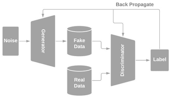
Figure 1.
A schematic of a Generative Adversarial Network, adapted from [21].
The generator is tasked with the generation of sample data by propagating a noise vector through its architecture to output data. Generated samples are classified by the discriminator as either real or fake [22]. The outcome of the discriminator is back-propagated into both sub-networks to improve their performance over multiple epochs.
A GAN is based on a game-theoretic scenario where the generator competes against the discriminator. The generator tries to minimise the discriminator loss while maximising its performance, and the opposite applies to the discriminator [21].
2.3. Mathematical Framework
The mathematical formulation of the GAN model employs an algorithmic mathematical framework that takes advantage of adaptable numerical transforms to generate data that are comparable to a set of target data. The generator input () is a random noise variable sampled from a normal distribution. The goal is iteratively to solve a transformation such that the cumulative distribution function (CDF) of the generator output () closely correlates with that of the target data [23]. This is expressed via Equation (1).
The discriminator output is a binary classification of whether the input that passed into it was real or fake; this is expressed in Equation (2). The network performance is quantified as a loss function and calculated as the cumulative expected value of the fake and real output, as expressed in Equation (3).
3. Methodology
3.1. System Overview
The designed system is composed of data acquisition, processing, frequency detection, and a Class-Conditioned Wasserstein GAN component with a gradient penalty loss. The participating subject is tasked with staring at an LCD that flashes at various frequencies, while trying to maintain a relatively constant respiratory rate, low movement, and posture to eliminate potential artefacts in the acquired data.
The EEG response of the subject to the flashing image is preprocessed, class-conditioned, and then passed to the WGAN for training and validation. Figure 2 illustrates the overall system set-up. The following sections detail the system specifications.
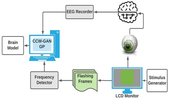
Figure 2.
Overview of the system for data acquisition and generation of the brain model.
3.1.1. Input
The input to the system is flashing green box video at 60 frames per second (FPS), displayed on the LCD with a refresh rate of 60 Hz. LCD monitors are convenient as they are widely available and have been shown to generate reliable SSVEP due to their constant refresh rate, contrast, and luminance [24].
Including more features in the input stimulus such as shapes, varying colour, and relative motion complicates the GAN design. Thus, the decision to use monochromatic visual stimuli reduces the complexity of the solution.
The frames i of the video are representative of a discrete-time signal generated at 60 Hz by the display. The input signal in this context is a periodic square wave such that a black frame is low and a green frame is high. Various frequencies are obtained by calculating the flashing period c.
Given a sampling frequency of 60 Hz, a 6 Hz flashing frequency would correspond to a frame span of 10. In this case, the flashing sequence would comprise five consecutive black frames and five green frames. Figure 3 illustrates the stimulus generation technique.
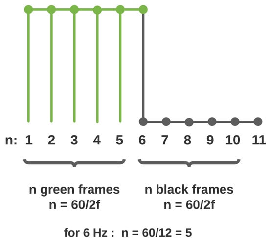
Figure 3.
Frequency Generation.
The minimum flashing period is two frames in duration. Hence, there is an upper limit of 30 Hz when generating flashing signals that may be displayed without aliasing as per the Nyquist sampling theorem. The experimental procedure makes use of 5, 6, 7.5, and 10 Hz flashing frequencies to demonstrate the concept and viability of the proposed model. The visual stimuli videos were generated with OpenCV [25] to ensure consistency and accuracy in the generation of each flashing visual stimulus.
3.1.2. Data Acquisition and Processing
Data acquisition was performed to obtain a subject’s real-world EEG data containing the SSVEP response when exposed to flashing visual stimuli. Two separate computers were used in the data acquisition process. One was used to display the visual stimuli to the participant, and another was connected to the EEG device to record neural responses. This configuration allows for each computer to direct specific tasks, which reduces the chance of information loss in data sampling.
Data acquisition was performed in a room in which the lighting was regulated. Of the total acquired data samples, half were obtained under low light conditions, and the other half were obtained under normal ambient lighting conditions. The darker conditions provided slightly better data; however, the data from both lighting conditions were used to train the GAN model to enable some model variance to lighting conditions.
The study participants were two of the authors, both of whom are males in the age group 20–30. The participants were seated a distance of 55–65 cm away from the LCD monitor during the experiment, which is within the ergonomic standards of viewing distance from a standard monitor [26]. Furthermore, the participants maintained a steady posture, low movement, and consistent respiration rates during data acquisition.
The g.tec HiAmp with active electrodes was used to record EEG activity, configured to sample at 256 Hz via the g.Recorder. The electrode placement corresponds to the parietal and occipital regions of the scalp as illustrated on the montage in Figure 4. Each measurement session lasted for 1 min in which the recording was delayed by 10 s to account for the transient eye adaptation period and to optimise for SSVEP signal acquisition.
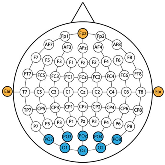
Figure 4.
EEG montage.
The eight channel acquired EEG data were passed through a fifth-order notch filter with a notch width of 0.01 Hz centred around 50 and 100 Hz to remove powerline noise. The signal was also filtered using a fifth-order bandpass filter with a passband of 1 Hz to 50 Hz to remove potential artefacts such as electromyographic signals (such as tempo-romandibular joint discharge) and electro-oculographic (eye blinks and movement) signals.
Data were collected as 1024 datapoints, sampled at 256 Hz across channels, which comprises 4 s batches.
The filtering processes yielded an overall settling time of approximately 1 s. Thus, the two ends of the recorded signals were cropped to remove preprocessing artefacts. Finally, an averaging kernel filter of size three was employed to increase the signal-to-noise ratio. The quality of the collected SSVEP data were visually assessed via the power spectral densities of each channel.
3.1.3. Frequency Detection
The frequency detection algorithm is a recurrent algorithm rather than a network. No intensive image processing is required as there is a clearly defined region of interest. Each three-channel frame is reduced to a three-channel vector that averages out the brightness of the frame. The three-channel vector is further reduced to a single averaged value that can be contrasted with 0 to detect whether an image is present.
The frequency detection takes in each frame brightness score and compares it with the previous frames score by regressing by a frame for a total period of 1 s. The frequency variable is incremented over the 1 s period every time the brightness score changes. Figure 5 illustrates this process.
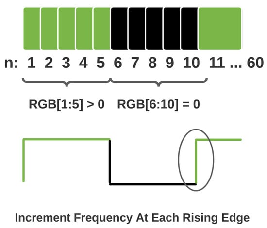
Figure 5.
Frequency detection.
This theoretically models the optic tract in the visual pathway by adopting the behaviour of retinal ganglion cells while processing visual potentials. The various specialised neurons in the retinal cell layers respond to the rate of change in action potentials by comparing current cell states to previous cell states.
3.1.4. Wasserstein Generative Adversarial Network
The GAN model described in Section 2.2 is modified to a WGAN model [27]. The diagram in Figure 6 illustrates the design modifications. Wasserstein distance is a method that calculates the difference between the real and generated data by computing the distances between the probability distributions of the real and fake data.
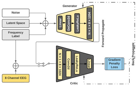
Figure 6.
CC WGAN GP.
The earth mover distance enables the discriminator to score the realness or fakeness of the data instead of performing binary classification. Therefore, in WGAN, the discriminator is named a Critic. WGAN is chosen over a regular GAN structure due to its floating-point loss value being back-propagated instead of binary-classification-based weight adjustment.
The intrinsic structure of the WGAN architecture also attempts to stabilise the training process by implementing a gradient penalty loss function to assign loss scores and prevent mode collapse. The model is further modified to be class-conditioned based on the detected frequency [27]. The conditioning is implemented in the form of label embedding using the output of the frequency detection algorithm.
The loss function for a WGAN is calculated as shown in Equation (4). A gradient penalty loss was introduced to avoid vanishing gradients during the WGAN training process, which requires the fine-tuning of sensitive hyperparameters. This penalty term is computed, as shown in Equation (5). is the real distribution, is the generated distribution defined by , and z is the random noise. is implicitly defined to uniformly sample along straight lines between pairs of points sampled from and .
3.2. Generator Design
3.2.1. Generator Architecture & Implementation
The generator architecture is adapted from work utilising GANs for EEG signal generation [14]. The input to the generator is a Gaussian noise signal projected onto a latent space vector with a default size of 1024.
The noise input generation is followed by an embedding function, with an embedding size that matches the length of the latent noise vector. Embedding class labels conditions the input for the various frequencies that are being investigated. The network architecture is coded to be dynamically resizable to enable the freedom to generate artificial data of various lengths.
Table 1 illustrates the architecture of the generator for an input feature size of 128 and output dimensions of (8, 1024). The linear layer is used to ensure that the model is fully connected. It also enables the variation of the latent noise length without disrupting the dimensional framework of the rest of the architecture. The output of the fully connected layer is a sequence that is resized such that its size reduces to the required output size via a series of convolutional layers.

Table 1.
Generator Architecture (BN: BatchNorm, *: Indicates variable size).
The hidden layers of the network are composed of three transposed 2D convolutions, and the output layer has a single regular 2D convolutional layer. The kernel size of the first two transpose convolutions is (1, 4) with a stride of (1, 2) and padding of (0, 1). Thereafter, the two consequent convolutional layers use a kernel size of (1, 3) with a stride of (1, 1) and padding of 0. This enables a balanced structure that up-samples the generated data length and down-samples the number of feature channels to 1 as shown in the Table 1.
The linear layer generates the sequences, which become the eight-channel EEG data, and the subsequent convolutional layers have rectangular kernel sizes spanning a single EEG channel. This prevents cross-channel contamination between the eight channels in the generated data.
The activation function for the input and hidden layers is leaky-relu preceded by a batch normalisation layer, which helps prevent vanishing and exploding gradients. The final layer is a tanh activation function to output samples ranging between 1 and −1. The regular GAN generator makes use of a sigmoid function instead, which outputs values ranging between 0 and 1. A potential alternative to the tanh activation is the ELU non-linear activation function. However, this may leave the model prone to negative exploding gradients.
3.2.2. Generator Training Process
The training process of the CC WGAN involves two stages, namely, critic training and generator training. The preprocessed training data are passed into the system by splitting up four sessions into batches of 1024 samples, corresponding to 4 s of EEG data. The batch division was implemented to achieve a fairly consistent power spectral density of each batch, as using smaller batch divisions causes large variance in the frequency content of the data due to the low signal-to-noise ratio.
The noise input is used to train the model over 100 epochs. Initially the noise with a label embedding is passed into the generator while its intrinsic weights are initialised to 0. While the generator produces some output, the critic is fed with a batch of training data with the same label embedding as the generator input so that its weights are appropriately updated before attempting to score the generator output. The generated data are then fed into the critic to measure the adversarial loss based on expression (5). The adversarial loss is then back-propagated to the critic to improve its performance. The critic is trained by iterating this process for each batch.
The generator is not trained as often as the critic. The critic should outperform the generator so that the training process is effective. If the critic can not accurately score the fake and real datasets, the generator will be trained with an incorrect back-propagated loss metric. This phenomenon gives rise to a concept known as the training ratio. The model uses a training ratio of five. Hence, generator back-propagation occurs once every five batches, whereas the critic back-propagation occurs every batch. The implementation of the architecture and the training process is carried out on Pytorch using the ADAM optimiser. The learning rate is , and momentum values are 0.5 and 0.9 for and , respectively.
3.3. Critic Design
3.3.1. Critic Architecture & Implementation
The critic receives input from a real EEG database and the output of the generator. The input dimensions are assumed to be an eight-channel EEG with a single feature channel for a duration of 1024 samples. The critic is designed to exhibit supervised learning by accepting label inputs as a second parameter to distinguish between the various classes of input. The received label is embedded into the input as an additional feature channel using an embedding layer with a size equivalent to the input dimensions.
The embedded input is passed through the rest of the critic architecture that consists of four convolutional layers and two fully connected layers.
Table 2 presents the various layers of the architecture along with their activation functions. The only batch normalisation occurs after the first convolutional layer to ensure that all the features extracted are normalised. This is important, since EEGs may have varying magnitudes across multiple channels.
Table 2.
Critic Architecture (*: Indicates variable size).
All the convolutional layers employ a constant kernel size of three, a stride of two, and a padding of one. The number of output features for each convolutional layer is double that of the input features of the signal. This structure was employed to reduce the length of the data. All the convolutional layers use the non-linear LeakyReLU activation functions.
The output of the final convolutional layer is flattened into a single dimension and fed into a fully connected layer. The fully connected layer, with a sequential output of length 1024, is passed into another LeakyReLU activation function.
The final fully connected layer is added to generate a score output of size one. The dimensional reduction is split between two linear layers to increase the number of learnable parameters at the output layer.
Unlike the discriminator in a typical GAN, the final layer of the critic does not contain a sigmoid activation function. The sigmoid activation function outputs either the values 0 and 1, which is a characteristic of a classifier that aligns with the goals of a GAN discriminator. A WGAN critic, however, does not classify, but scores the realness or fakeness of the input data.
3.3.2. Critic Training Process
The critic must be trained simultaneously with the generator. However, in order for it to distinguish between real and fake data, the critic must outperform the generator. Various applications have varying frequencies at which the critic is trained relative to the generator, known as a training ratio.
The project uses a training ratio of 5, meaning that the generator is trained every 5 batches whereas the critic is trained at each batch.
4. Results
The machine learning model was trained and tested for the target frequencies 5 Hz, 6 Hz, and 7.5 Hz. For each target frequency, 25 batches of 1024 data samples were used to train and test the model. The training process used 23 training batches and 1 validation batch and ran for 100 epochs.
The size of the validation and test sets were limited to maximise the size of the training data. The split ratio can be decreased to increase the number of batches over each epoch. However given that EEG data often have a small signal-to-noise ratio, using smaller data segments per batch decreases the signal-to-noise ratio even further.
The trained model was then used to generate sample sets, which were compared against a test batch to obtain accuracy measures. It should be noted that the test batch was unseen, in that it did not form part of the training set for unbiased comparison.
The model performance was evaluated by using various accuracy measures, and the training process was evaluated through the adversarial and the gradient penalty loss. The generated results were also visually assessed through time and frequency domain analysis.
4.1. Training Results
Two metrics were utilised to assess the performance of the WGAN GP model: the adversarial and the gradient penalty loss. The gradient loss starts from 0.01 and is maximised approximately to 11,106 by the end of the 100 epochs. The adversarial loss appears to be minimised from 9.08 to −8493 over the training period. The losses do not accurately reflect the accuracy of the model, but indicate whether the model is behaving as expected throughout the training process.
The adversarial loss provides a measure of the discrepancy between the real and fake data distributions and further serves as a training criterion [28]. Hence, a favourable adversarial loss is expected to be a diverging measure. In this case, the training results seem to follow this favourable trend, indicating that the model could potentially be improved with longer training epochs. As a result, the outcome of the training process shows that a CC WGAN with a gradient penalty loss can be used to create a model capable of mimicking the visual response of the human brain and of generating EEG data.
4.2. Time and Frequency Analysis
Figure 7 illustrates the power spectral density (PSD) and the time series of a randomly selected generated SSVEP signal plotted against a real sample at frequencies of 6 Hz, 7.5 Hz, and 5 Hz.
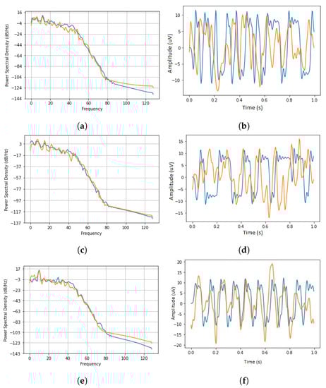
Figure 7.
The time-series and power spectral density for 6 Hz, 7.5 Hz, and 5 Hz frequencies. The orange trace is the real data and the blue trace demonstrates the generated SSVEP signal. (a) 6 Hz SSVEP PSD. (b) 6 Hz SSVEP Time-Series. (c) 7.5 Hz SSVEP PSD. (d) 7.5 Hz SSVEP Time-Series. (e) 5 Hz SSVEP Time-Series. (f) 5 Hz SSVEP PSD.
The time series of the generated sample exhibits a periodic nature as a result of learning the key repeated features of the source (real) dataset. The general periodic time-series pattern observed from the generated dataset closely resembles the pattern that is expected to be observed for an SSVEP response [7]. Since the time-series signal plots are shown for 1 s, the number of repeated amplitude spikes directly correspond to the flashing frequency.
Although the time series of the generated dataset shows variation in amplitude sizes, it should be noted that, through training, the model has managed to learn the key feature and, therefore, the inconsistencies and the outliers observed in the real signal are discarded while the key features across all batches are conserved.
The PSD of the generated samples is drawn using a Hanning window and a sampling frequency of 256 Hz. At each epoch during training, the PSDs are saved on the tensorboard, along with the adversarial and gradient losses, to track the training progress.
In Figure 7, orange curves represent real data and blue curves represent artificial data. The PSD plots of the real dataset for each flashing frequency show a large spike at the specific flashing frequency and its harmonics.
Comparing the generated to the real datasets shows that the model has managed to closely trace the PSD of the real data. This is especially true when observing the critical frequency that corresponds to the flashing frequency. At this frequency, the PSD of the generated and the real dataset closely correlate with each other. This is due to the prominent presence of this key frequency within the real dataset compared to the inconsistencies across the rest of the spectrum. The minor variations in the generated power spectra are tolerable due to the variations in the training data and indicate that the model is not prone to overfitting.
4.3. Quantifying Model Performance
Testing was performed in order to quantify the ability of the model to represent the SSVEP stimulus frequency in the output signal. These tests involved quantifying the accuracy of the generated data using the Average Cross-Channel Accuracy and the Average Spectral Accuracy.
4.3.1. Average cross Channel Accuracy
The model generated 100 samples of data for each frequency on which it was trained. The cross spectral density per EEG channel was determined between each generated set and the unseen test set. The peak correlations for each EEG channel were then determined, and observed to see whether they fall within a given tolerance of the input stimulus frequency and its first harmonic. Finally, the percentage accuracy for each EEG channel in the generated set was calculated as the total number of peak channel correlations out of the total generated samples that fit the aforementioned criteria.
The results of this performance measure are presented in Table 3 for a tolerance of 1 Hz. The Harmonic Index relates to the signal’s fundamental frequency and its first harmonic, as per the equation , in which indicates the fundamental frequency (SSVEP frequency in this case), and i indicates the harmonic index.
Table 3.
Model’s performance in generating signals with SSVEP features in response to a given stimulus when evaluated against unseen test data with a 1 Hz tolerance.
The performance of the model is expressed as the average cross-channel percentage accuracy for the fundamental frequency and its first harmonic at the bottom, giving an overall indication of the model’s ability to generate signals with SSVEP frequencies dominant for the given frequency stimulus. For most of the runs, the model performance is above 80%, and for many of the runs it is 100%. This indicates the model’s ability to recreate the SSVEP frequency as the dominant frequency in the output when compared with unseen test data obtained with the same stimulus.
4.3.2. Average Spectral Accuracy
This involved separately quantifying the accuracy of the training data and generated data, then comparing them against each another. Given a test SSVEP set with a target frequency f, the average spectral accuracy is measured as the average number of peaks in the power spectral density that are present within a given tolerance range of the target frequency, averaged out across all channels. Various tolerance values were used for the assessment to indicate the model performance.
Comparing the accuracy of the training data and generated data for the same target frequency can provide an insight as to how well the model performs in situations where the training data may be inaccurate. Figure 8 serves to illustrate the tolerances in the training and generated sets (in which 100 batches were generated in each). The training and generated data PSDs are evaluated to determine whether they fall into given tolerance ranges for each frequency.
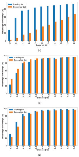
Figure 8.
Percentages falling within tolerances in the training and generated sets blended over the fundamental and 1st harmonic. (a) 5 Hz SSVEP. (b) 6 Hz SSVEP. (c) 7.5 Hz SSVEP.
It is evident from the Figure 8 that there is a tolerance of approximately 0.5 Hz in a fair proportion of the training data. The generated data show a similar tolerance for 100 generated batches; however, the performance for 5 Hz is considerably poorer than the other two frequencies, which more closely match the tolerance of the training data.
Performance changes with a lower tolerance. For instance, results for a smaller tolerance of 0.2 Hz are presented in Table 4. This table presents data that are aggregated across all channels.
Table 4.
Evaluating model performance by calculating average spectral accuracy across all channels for various tolerances.
5. Discussion
The investigation results indicate that the proposed solution can replicate the major features of an SSVEP signal. However, the design is limited to a specific set of constraints and assumptions. The following sections critically review the study, suggesting potential applications, and providing recommendations for future work.
The model has successfully demonstrated the ability to model a neurological process, from stimulus to EEG from data. The behaviour of the system with test data indicates that the model behaves similarly to the human brain’s visual processing system when stimulated with SSVEP signals. This indicates that a neurological process can be encapsulated within a model from the data. The system then forms a model of the visual system’s behaviour, behaving similarly to the human visual system under stimulus. Forming input/output models of the brain’s behaviour may help to understand the properties of the brain.
The model has some limitations. It was developed for a specific kind of visual stimulus from an LCD. The flashing image sequences are monochromatic, with a single object as the region of interest. Although this limitation simplifies the complexity, it is also limited to one specific type of stimulus. Modifying the input component of the design would require a complex label encoding that could significantly increase the model complexity. Increasing the learnable parameters of the model requires a longer training duration and higher computational capacity. The output of the generator model is normalised and the high-frequency components are often not attenuated as effectively across the convolution layers.
An intrinsic low-pass filter is implemented at the output of the model to attenuate frequency components above 50 Hz. The filter is also used during training to reduce the high-frequency processing requirements. These components impact the probability distributions that are measured by the model when scoring the data.
The current model uses zero-weight initialisation for convolutional layers and uniform weight kernels for deconvolutional layers. The model could be further improved by increasing the training epochs, and by varying the training hyper-parameters to observe their impact on the generated results and on the performance of the model. In addition, exploring various weight initialisers could increase model performance.
5.1. Potential Applications
The model is an offline system that requires collected data, and creating a real-time model is unnecessary because the generated data are intended for EEG data augmentation. The model generates artificial EEG data that could ultimately be used to train a BCI based system.
The produced model can also be used for fundamental research, since symmetry is created between the brain’s visual response under SSVEP conditions and the model’s response when exposed to SSVEP-generating signals. Once an external model of a biological system is obtained, this allows for further study in interfacing with external systems. It also allows for an understanding of components of the system, which may allow for artificial components to be generated and tested. Furthermore, the behaviour of neural pathways can be modelled using machine learning techniques from neurological data.
Another potential application of this work is in assistive devices. One such application is in controlling a variety of external systems, such as enabling wheelchair motion by analysing and mapping various SSVEP signals.
5.2. Recommendations for Future Work
The system subcomponents should be evaluated to identify the shortcoming of the overall system. The LCD monitor is used as an input to the system; although proven to generate reliable SSVEP response, this would be improved by using LED, which has been known to generate higher-quality SSVEP. However, this would complicate the process in several ways. An external camera is required to capture the flashing pattern of the LEDs with 60 FPS due to the system input of a flickering video. In addition, since LEDs do not offer the already-present eye-safety features of LCD monitors, the LED’s light-intensity and frequency parameters had to be carefully tuned for eye safety. Therefore, to simplify the process, the LCD monitor was utilised.
The frequency detection sub-component may be improved to enable detection of the frequency component of more complex image patterns, such as a flickering chequerboard or circular shapes. Furthermore, an additional feature may be implemented where a camera-recorded flashing frequency could be used as input. In this case, an algorithm must first detect the region of interest and then perform slightly more complex image-processing techniques to detect the flashing frequency. However, the implemented frequency detection algorithm was developed to perform sufficiently for the video input that is presented to the subjects of this research investigation.
During the data acquisition process, the EEG data could be recorded for a shorter duration than 1 min (for example, 30 s). This would for allow the subjects to fixate attention on the flashing frequency without losing focus due to eye fatigue. Furthermore, a shorter sampling duration would contribute to a higher signal-to-noise ratio as it would include more desirable features, as losing attention creates undesirable data, including neural artefacts.
The trained model can be improved by taking additional data from a broader group of subjects. This would allow for the model to learn the general key features that appear in different test subjects, allowing for a more generalised unbiased model to be obtained. The model could also be improved through extended training duration. However, this requires more data and increased computation.
5.3. Ethical & Safety Concerns
There are several ethical considerations in the data acquisition phase of the study. To minimise the risk of seizure, the subjects participating in the study had declared that they had no medical history of photosensitive epilepsy. Even though a commercial LCD was used in the study, and is assumed to operate within the eye-safety range, the screen brightness was capped at 70% to further minimise eye health risk.
Each recording session was followed by a 5 min break to prevent the eye from experiencing high fatigue due to exposure to flashing images.
The recording device only initiated the recording session once unnecessary background processes were terminated, as instructed by the g.tec HiAmp user guide. This is a safety measure taken to prevent electrode current discharge onto the scalp while measuring EEG activity.
6. Conclusions
A model capable of mimicking the visual pathway of the human brain under SSVEP stimulation has is generated. The model is capable of generating signals that are similar in nature to those of the brain when it is exposed to flickering light at a given frequency, which induces an SSVEP response. This model is an input/output view of the brain and can be used for data augmentation and generation, understanding the brain’s behaviour, better interfacing the brain with external devices, understanding individual components of the visual processing system, and demonstrating how neural pathways can be modelled using machine learning.
EEG is a means of measuring brain activity, and it is an important component of BCI systems. Large sets of EEG data are often required in training BCI systems to interpret brain activity. The complexities of EEG data collection makes the acquisition a challenging task. Hence, a class conditioned WGAN model with a gradient penalty loss is used to demonstrate a viable method of EEG data generation/augmentation.
The proposed model consists of a critic and a generator. The generator replicates key features found in the acquired data by using the output of the critic as a training criterion. Once the model is trained for 25 batches of four-second EEG data over 100 epochs, it generates artificial EEG signals with power spectral densities that closely correlate with that of the real EEG data for the observed human SSVEP response.
The obtained results indicate that the proposed design is is a viable solution to the generation of brain signals as recorded on EEG with real-world stimuli. The model is effectively an input–output model of the visual pathway, mapping a specific visual stimulus to an expected SSVEP response, as recorded by EEG. This creates the concept of symmetry between the human brain’s behaviour under SSVEP stimuli as measured by EEG and the output of the model due to the same stimuli.
Author Contributions
S.E.K.: software, formal analysis, investigation, writing—original draft preparation; M.M.K.: software, formal analysis, investigation, writing—original draft preparation; A.P.: conceptualisation, methodology, supervision, project administration, writing—review and editing. All authors have read and agreed to the published version of the manuscript.
Funding
This research received no external funding.
Institutional Review Board Statement
The data were collected with institutional review board clearance by the Human Research Ethics Committee (Medical) at the University of the Witwatersrand, Johannesburg (clearance number M170839).
Informed Consent Statement
Informed consent was obtained from all subjects involved in the study.
Data Availability Statement
Data available on request.
Conflicts of Interest
The authors declare no conflict of interest.
References
- Abdulkader, S.N.; Atia, A.; Mostafa, M.S.M. Brain computer interfacing: Applications and challenges. Egypt. Inform. J. 2015, 16, 213–230. [Google Scholar] [CrossRef] [Green Version]
- Koch, C.; Buice, M.A. A Biological Imitation Game. Cell 2015, 163, 277–280. [Google Scholar] [CrossRef] [PubMed] [Green Version]
- Blohm, G.; Kording, K.P.; Schrater, P.R. A How-to-Model Guide for Neuroscience. Eneuro 2020, 7, 2–3. [Google Scholar] [CrossRef]
- Guger, C.; Millan, J.d.R.; Mattia, D.; Ushiba, J.; Soekadar, S.R.; Prabhakaran, V.; Mrachacz-Kersting, N.; Kamada, K.; Allison, B.Z. Brain-computer interfaces for stroke rehabilitation: Summary of the 2016 BCI Meeting in Asilomar. Brain-Comput. Interfaces 2018, 5, 41–57. [Google Scholar] [CrossRef]
- Lebedev, M.A.; Nicolelis, M.A.L. Brain-Machine Interfaces: From Basic Science to Neuroprostheses and Neurorehabilitation. Physiol. Rev. 2017, 97, 767–837. [Google Scholar] [CrossRef] [PubMed]
- Lin, J.S.; Shieh, C.H. An Ssvep-Based Bci System and its Applications. Int. J. Adv. Comput. Sci. Appl. 2014, 5, 54–55. [Google Scholar] [CrossRef] [Green Version]
- Norcia, A.M.; Appelbaum, L.G.; Ales, J.M.; Cottereau, B.R.; Rossion, B. The steady-state visual evoked potential in vision research: A review. J. Vis. 2015, 15, 4. [Google Scholar] [CrossRef] [Green Version]
- Rao, R.P. Brain-Computer Interfacing: An Introduction; Cambridge University Press: Cambridge, UK, 2013. [Google Scholar]
- Jackson, A.F.; Bolger, D.J. The neurophysiological bases of EEG and EEG measurement: A review for the rest of us. Psychophysiology 2014, 51, 1061–1071. [Google Scholar] [CrossRef]
- Bin, G.; Gao, X.; Yan, Z.; Hong, B.; Gao, S. An online multi-channel SSVEP-based brain computer interface using a canonical correlation analysis method. J. Neural Eng. 2009, 6, 046002. [Google Scholar] [CrossRef]
- Liu, B.; Huang, X.; Wang, Y.; Chen, X.; Gao, X. BETA: A Large Benchmark Database Toward SSVEP-BCI Application. Front. Neurosci. 2020, 14, 627. [Google Scholar] [CrossRef]
- Zhang, Q.; Liu, Y. Improving brain computer interface performance by data augmentation with conditional deep convolutional generative adversarial networks. arXiv 2018, arXiv:1806.07108. [Google Scholar]
- Corley, I.A.; Huang, Y. Deep EEG super-resolution: Upsampling EEG spatial resolution with generative adversarial networks. In Proceedings of the 2018 IEEE EMBS International Conference on Biomedical & Health Informatics (BHI), Las Vegas, NV, USA, 4–7 March 2018; IEEE: Hoboken, NJ, USA, 2018; pp. 100–103. [Google Scholar]
- Hartmann, K.G.; Schirrmeister, R.T.; Ball, T. Generative adversarial networks for brain signals. arXiv 2018, arXiv:1806.01875. [Google Scholar]
- Salakhutdinov, R. Learning deep generative models. Annu. Rev. Stat. Its Appl. 2015, 2, 361–385. [Google Scholar] [CrossRef] [Green Version]
- Goodfellow, I.; Pouget-Abadie, J.; Mirza, M.; Xu, B.; Warde-Farley, D.; Ozair, S.; Courville, A.; Bengio, Y. Generative adversarial nets. Adv. Neural Inf. Process. Syst. 2014, 27, 1–3. [Google Scholar] [CrossRef]
- Daya, R.N.; Dukes, M.N.; Pantanowitz, A. The brain as a network cable: Transmission of a modulated optical signal between two computers via the human brain. Inform. Med. Unlocked 2020, 21, 100490. [Google Scholar] [CrossRef]
- Ding, J.; Sperling, G.; Srinivasan, R. Attentional modulation of SSVEP power depends on the network tagged by the flicker frequency. HHS Author Manuscr. 2007, 16, 1016–1029. [Google Scholar] [CrossRef]
- Watson, A.B. A formula for human retinal ganglion cell receptive field density as a function of visual field location. J. Vis. 2014, 14, 1–17. [Google Scholar] [CrossRef] [Green Version]
- Gupta, M.; Bordoni, B. Visual Pathway; StatPearls: Treasure Island, FL, USA, 2021. [Google Scholar]
- Brownlee, J. A Gentle Introduction to Generative Adversarial Networks (GANs). Retrieved 2019, 17, 2019. [Google Scholar]
- Rocca, J. Understanding Generative Adversarial Networks (GANs). Medium 2019, 7, 20. [Google Scholar]
- Aznan, N.K.N.; Atapour-Abarghouei, A.; Bonner, S.; Connolly, J.D.; Al Moubayed, N.; Breckon, T.P. Simulating brain signals: Creating synthetic eeg data via neural-based generative models for improved ssvep classification. In Proceedings of the 2019 International Joint Conference on Neural Networks (IJCNN), Budapest, Hungary, 14–19 July 2019; pp. 1–8. [Google Scholar] [CrossRef] [Green Version]
- Cecotti, H.; Volosyak, I.; Gräser, A. Reliable visual stimuli on LCD screens for SSVEP based BCI. In Proceedings of the 2010 18th European Signal Processing Conference, Aalborg, Denmark, 23–27 August 2010; IEEE: Hoboken, NY, USA, 2010; pp. 919–923. [Google Scholar]
- Bradski, G. The OpenCV Library. Dr. Dobb’s J. Softw. Tools 2000, 25, 120–123. [Google Scholar]
- Woo, E.; White, P.; Lai, C. Ergonomics standards and guidelines for computer workstation design and the impact on users’ health—A review. Ergonomics 2016, 59, 464–475. [Google Scholar] [CrossRef] [PubMed]
- Arjovsky, M.; Chintala, S.; Bottou, L. Wasserstein GAN. arXiv 2017, arXiv:1701.07875. [Google Scholar]
- Dong, H.W.; Yang, Y.H. Towards a Deeper Understanding of Adversarial Losses under a Discriminative Adversarial Network Setting. arXiv 2019, arXiv:1901.08753. [Google Scholar]
Publisher’s Note: MDPI stays neutral with regard to jurisdictional claims in published maps and institutional affiliations. |
© 2022 by the authors. Licensee MDPI, Basel, Switzerland. This article is an open access article distributed under the terms and conditions of the Creative Commons Attribution (CC BY) license (https://creativecommons.org/licenses/by/4.0/).