Regularity and Travelling Wave Profiles for a Porous Eyring–Powell Fluid with Darcy–Forchheimer Law

Abstract

The goal of this study is to provide analytical and numerical assessments to a fluid flow based on an Eyring–Powell viscosity term and a Darcy–Forchheimer law in a porous media. The analysis provides results about regularity, existence and uniqueness of solutions. Travelling wave solutions are explored, supported by the Geometric Perturbation Theory to build profiles in the proximity of the equation critical points. Finally, a numerical routine is provided as a baseline for the validity of the analytical approach presented for low Reynolds numbers typical in a porous medium.

1. Introduction

Transport processes in porous media are typically given in several applications: mechanics, electrochemistry, metallurgic and geophysics, to cite some. In 1856, Darcy [1] provided a mathematical relation to study the fluid dynamics involved in porous media, particularly, water flows in sand beds.

The flow of a fluid in a porous medium typically occurs under low Reynolds numbers due to the interstitial structure of these kind of media. To increase the Reynolds numbers, it is required to enlarge the values of pressure gradients in the medium, i.e., to account for a steep pressure distribution. This fact improves turbulent mechanisms in the fluid, making the Darcy‘s law vague. Consequently, and to increase modelling accuracy in the mentioned circumstances, first Forchheimer in 1901 [2], and later Jaeger in 1956 [3], proposed empirical relations between the velocity and the hydraulic gradient in a turbulent flow. Currently, other modelling strategies are available. For example, in [4], analytical and numerical solutions were provided to model in shallow water. To this end, the $(G^{\prime }/G)—$expansion method was considered to obtain solutions to the classical Gardner equation, modified Korteweg–de Vries equation, and generalized Korteweg–de Vries equation. Afterward, the numerical approach allowed us to compare with the analytical findings.

Based on the studies in [2,3], the Darcy’s law was renamed as Darcy–Forchheimer’s principle by Mustak in [5] and Ward in [6]. Note that the mentioned formulations were considered for Newtonian fluids. Nonetheless, the Darcy–Forchheimer‘s law has been employed for non-Newtonian fluids as well (the reader is referred to [7,8,9,10] and references there for a wider scope).

There exist plenty of non-Newtonian fluids in the literature, but particularly, we focus our analysis on the Eyring–Powell fluid flow. This model allows us to describe the shear stress and the associated viscosity based on the kinetic theory of liquids. This underlying theory is robust enough to provide a kinematic condition describing the viscosity terms. In addition, and as it will be described afterwards in the governing equation, the fluid is assumed to flow in a porous medium given by a Darcy–Forchheimer law in independent term. A similar hybrid Eyring–Powell and Darcy–Forchheimer flow has been explored in [11] to model a fluid in a stratified stretching sheet embedded in a porous medium. In this mentioned study, numerical solutions, supported by a Chebyshev spectral method, are obtained to the set of non-linear equations describing the flow under study.

The Eyring–Powell fluid model has been considered to model flow profiles in magnetohydrodynamics (MHD). Akbar [12] studied solutions for a two dimensional MHD fluid. In addition, Hina [13] analysed a MHD Eyring–Powell fluid with heat transfer. Later, Bhatti et al. [14] considered a permeable stretching surface for an MHD flow and made an analysis involving heat transfer. Finally, the reader is referred to the set of papers [15,16,17,18,19,20] for further analysis related with Eyring–Powell fluids. Note that other kinds of non-homogeneous diffusion (not supported by the Eyring–Powell conceptions) have been considered in [21] for a Darcy–Forchheimer flow.

As it will be described, the present study provides travelling wave solutions. In this regard, and in the search of analytical profiles to non-Newtonian fluids, the studies [22,23,24] provide important achievements. In our case, the convergence and stability results in the travelling wave profiles are provided by a Geometric Perturbation approach and are validated by a numerical exercise using the module bvp4c in Matlab. Note that the numerical approach and the use of the function bvp4c have been previously employed in fluid modelling. In [25], the authors provided a modelling analysis about the impact of thermophoretic particle deposition and magnetic dipole in the flow of a Maxwell liquid over a stretching sheet. To this end, they used a numerical scheme based on a Runge–Kutta–Fehlberg 45 (RKF 45) process with shooting technique in ODEs. The authors in [26] employed the bvp4c function to solve a bioconvection flow of Sisko nanofluid confined by a stretched surface. Some other studies in MHD flows made use of advanced numerical analysis: the authors in [27] analysed a mesh-free weak-strong (MWS) method to provide solutions for a MHD flow in a pipe with different geometries and with arbitrary conducting walls. In [28], a meshless local Petrov–Galerkin method was used to search for solutions in an unsteady MHD flow for different values in the wall conductivity and for different Hartmann numbers. Further, in [29], an MHD flow was solved by a combination of finite volume method and spectral techniques. Another novel numerical analysis was provided in [30] where Crank-–Nicolson schemes supported by energy methods were employed to study the convergence and stability of the solutions.

The article structure is as follows: Firstly, a discussion about the fluid model proposed is introduced. Afterward, regularity of solutions is explored. Profiles of solutions are obtained based on the theory of travelling waves and the Geometric Perturbation Theory. Finally, a numerical process aims at validating the analytical approach proposed.

Fluid Model Principles

To start with, assume a one-dimensional, incompressible, unsteady and electrically conducting Eyring–Powell fluid. The velocity field is given by $\overrightarrow{V}=V\left(v_1\left(y,t\right),0,0\right),$ where $v_1\left(y,t\right)$ is the first velocity component depending of a transverse direction y. The geometry under study can be described as a big porous media with volume V and porous structures of typical size l, such that $V^{\frac{1}{3}}\gg l$. Given any interstitial distribution in the medium, a certain initial velocity is given as it will be introduced. The intention is to characterize the evolution of the velocity profile flowing through the $x—$axis and while varying with the transversal direction y. The hypothesis of a one dimensional flow is typical in flowing principles of pipes of stretching surfaces (see [31] for a MHD fluid flowing along rectangular and circular pipes).

The continuity equation and constitutive equation for Eyring–Powell fluid are given by:

$$div\overrightarrow{V}=0,$$

(1)

and:

$$\rho \frac{d\overrightarrow{V}}{dt}=div\overrightarrow{A}+\overrightarrow{J}\times \overrightarrow{B},$$

(2)

where $\rho$ is the fluid density, $\overrightarrow{J}$ is the current density, $\overrightarrow{B}$ is the magnetic field and $\overrightarrow{A}$ is given by

$$\overrightarrow{A}=-p\overrightarrow{I}+{\tau }_{ij},$$

(3)

$$div\overrightarrow{B}=0,curl\overrightarrow{B}={\mu }_1\overrightarrow{j},curl\overrightarrow{E}=-\frac{\partial \overrightarrow{B}}{\partial t}$$

(4)

$$\overrightarrow{J}=\sigma \left(\overrightarrow{E}+\overrightarrow{V}\times \overrightarrow{B}\right),$$

(5)

where p is pressure the pressure distribution, ${\tau }_{ij}$ is the shear stress tensor, $\overrightarrow{I}$ is the identity tensor, ${\mu }_1$ the magnetic permeability, $\overrightarrow{E}$ is the electric field and $\sigma$ is the electrical conductivity. The magnetic field can be expressed as: $\overrightarrow{B}={\overrightarrow{B}}_0+\overrightarrow{b}$ where ${\overrightarrow{B}}_0$ and $\overrightarrow{b}$ are the imposed and induced magnetic fields, respectively. In addition, the shear stress tensor ${\tau }_{ij}$ for an Eyring–Powell fluid model is given by (refer to [16]):

$${\tau }_{ij}=\mu \frac{\partial v_i}{\partial x_j}+\frac{1}{\beta }{sinh}^{-1}\left(\frac{1}{d_1}\frac{\partial v_i}{\partial x_j}\right),$$

(6)

where $\mu$ dynamic viscosity, $\beta$ and $d_1$ are the characteristics of Powell–Eyring model and $v_i$ the velocity component for $i=1,2,3$. Considering:

$${sinh}^{-1}\left(\frac{1}{d_1}\frac{\partial v_i}{\partial x_j}\right)\cong \frac{1}{d_1}\frac{\partial v_i}{\partial x_j}-\frac{1}{6}{\left(\frac{1}{d_1}\frac{\partial v_i}{\partial x_j}\right)}^3,\left|\frac{1}{d_1}\frac{\partial v_i}{\partial x_j}\right|\le 1.$$

The governing equation for $i=1$ in the absent of induced magnetic field can be written as (refer to [15,16,17]):

$$\frac{\partial v_1}{\partial t}=-\frac{1}{\rho }\frac{dP}{dx}+\left(\nu +\frac{1}{\beta C_1\rho }\right)\frac{{\partial }^2{v}_1}{\partial y^2}-\frac{1}{2\beta C_1^3\rho }{\left(\frac{\partial v_1}{\partial y}\right)}^2\frac{{\partial }^2{v}_1}{\partial y^2}-\frac{\sigma B_0^2{v}_1}{\rho }-\frac{\nu v_1}{K}-\frac{v_1^2}{K_1},$$

(7)

where $\nu =\frac{\mu }{\rho }$ is the kinematic viscosity, K is the permeability (hydraulic conductivity) of the porous medium, $K_1$ is the inertial permeability, $C_1$ is a fluid characteristic constant and $B_0$ refers to the magnitude of the imposed magnetic field as describe above. Let us introduce non-dimensional quantities (refer to [32]) as follows:

$$\begin{array}{ccc}\hfill v_1^{*}& =& \frac{v_1}{U_0},x^{*}=\frac{x}{L},y^{*}=\frac{y}{L},t^{*}=\frac{U_0}{L}t,P^{*}=\frac{P}{\rho U_0^2},A=\frac{1}{\beta C_1\rho },\hfill \\ \hfill ϵ& =& \frac{U_0}{2\rho \beta C_1^3{L}^3},F=\frac{U_0}{K},G=\frac{U_0^2}{K_1}.\hfill \end{array}$$

(8)

Substitute (8) into into Equation (7) (ignoring ${}^{*}$ for simplicity):

$$\frac{\partial v_1}{\partial t}=-\frac{dP}{dx}+\frac{1}{R_e}\left(1+A\right)\frac{{\partial }^2{v}_1}{\partial y^2}-ϵ{\left(\frac{\partial v_1}{\partial y}\right)}^2\frac{{\partial }^2{v}_1}{\partial y^2}-\left(\frac{M^2}{R_e}+F\right)v_1-G{v}_1^2,$$

(9)

where $R_e=\frac{U_{0}L}{\nu }$ is the Reynolds number and $M=B_{0}L\sqrt{\frac{\sigma }{\rho \nu }}$ is the Hartmann number. Now, differentiate the Equation (9) with regards to x, so that:

$$-\frac{d^{2}P}{d{x}^2}=0,-\frac{dP}{dx}=K_2.$$

After using the value of $-\frac{dP}{dx}$ in Equation (9):

$$\frac{\partial v_1}{\partial t}=K_2+\frac{1}{R_e}\left(1+A\right)\frac{{\partial }^2{v}_1}{\partial y^2}-ϵ{\left(\frac{\partial v_1}{\partial y}\right)}^2\frac{{\partial }^2{v}_1}{\partial y^2}-\left(\frac{M^2}{R_e}+F\right)v_1-G{v}_1^2,$$

(10)

As pointed previously, it is required to introduce a general initial velocity distribution that is related with the interstitial structure of the medium. Mathematically, this is considered as follows:

$$v_1(y,0)=v_{10}\left(y\right)\in L^1\left(R\right)\cap L^{\infty }\left(R\right),$$

(11)

where $v_1\to 0^{+}$ at the pseudo-boundary in $\left|y\right|\to \infty$ and $v_{10}\left(y\right)$ refers to the mentioned initial velocity distribution.

2. Existence and Uniqueness of Solutions

Let us consider a test function ${\varphi }_1\in C^{\infty }\left(R\right)$ such that for $0<\tau <t<T:$

$$\begin{array}{ccc}\hfill \underset{R}{\int }{v}_1\left(t\right){\varphi }_1\left(t\right)dy& =& \underset{R}{\int }{v}_1\left(\tau \right){\varphi }_1\left(\tau \right)dy+\underset{\tau }{\stackrel{t}{\int }}\underset{R}{\int }{v}_1\frac{\partial {\varphi }_1}{\partial s}dyds+A_1\underset{\tau }{\stackrel{t}{\int }}\underset{R}{\int }{\varphi }_{1}dyds\hfill \\ & & +\frac{1}{R_e}\left(1+A\right)\underset{\tau }{\stackrel{t}{\int }}\underset{R}{\int }{v}_1\frac{{\partial }^2{\varphi }_1}{\partial y^2}dyds+\frac{ϵ}{3}\underset{\tau }{\stackrel{t}{\int }}\underset{R}{\int }{\left(\frac{\partial v_1}{\partial y}\right)}^3\frac{\partial {\varphi }_1}{\partial y}dyds\hfill \\ & & -\left(\frac{M^2}{R_e}+F\right)\underset{\tau }{\stackrel{t}{\int }}\underset{R}{\int }{v}_1{\varphi }_{1}dyds.-G\underset{\tau }{\stackrel{t}{\int }}\underset{R}{\int }{v}_1^2{\varphi }_{1}dyds.\hfill \end{array}$$

(12)

Assume a finite $r_0\in R^{+}$ and define a ball $B_r$ accordingly, such that $r\gg r_0$. The following equation is defined in $B_r\times \left[0,T\right]$:

$$v_1\frac{\partial {\varphi }_1}{\partial s}+A_1{\varphi }_1+\frac{1}{R_e}\left(1+A\right)v_1\frac{{\partial }^2{\varphi }_1}{\partial y^2}+\frac{ϵ}{3}{\left(\frac{\partial v_1}{\partial y}\right)}^3\frac{\partial {\varphi }_1}{\partial y}-\left(\frac{M^2}{R_e}+F\right)v_1{\varphi }_1-G{v}_1^2{\varphi }_1=0,$$

(13)

with the following boundary and initial like conditions:

$$0<\frac{\partial {\varphi }_1}{\partial y}={\varphi }_1\ll 1,$$

$$v_1\left(y,0\right)=v_{10}\left(y\right).$$

The following Theorem shows the existence of solutions to the defined problem (13).

Theorem 1.

Given $v_{10}\left(y\right)\in L^1\left(R\right)\cap L^{\infty }\left(R\right)$, then the solution is bounded for all $\left(y,t\right)\in B_r\times \left[\tau ,T\right]$ with $r\gg 1.$

Proof. 

Consider $\zeta \in R^{+}$. The following cut-off function is defined:

$${\psi }_{\zeta }\in C_0^{\infty }\left(y,t\right),0\le {\psi }_{\zeta }\le 1,$$

$${\psi }_{\zeta }=1\mathrm{in}{B}_{r-\zeta },{\psi }_{\zeta }=0\mathrm{in}R-B_{r-\zeta },$$

so that:

$$\left|\frac{\partial {\psi }_{\zeta }}{\partial \zeta }\right|=\frac{B_c}{\zeta },$$

Multiplying the Equation (13) by ${\psi }_{\zeta }$ and integrating in $B_r\times \left[\tau ,T\right],$ we obtain:

$$\underset{\tau }{\stackrel{t}{\int }}\underset{B_r}{\int }{v}_1\frac{\partial {\varphi }_1}{\partial s}{\psi }_{\zeta }dyds+A_1\underset{\tau }{\stackrel{t}{\int }}\underset{B_r}{\int }{\varphi }_1{\psi }_{\zeta }dyds+\frac{1}{R_e}\left(1+A\right)\underset{\tau }{\stackrel{t}{\int }}\underset{B_r}{\int }{v}_1\frac{{\partial }^2{\varphi }_1}{\partial y^2}{\psi }_{\zeta }dyds$$

$$+\frac{ϵ}{3}\underset{\tau }{\stackrel{t}{\int }}\underset{B_r}{\int }{\left(\frac{\partial v_1}{\partial y}\right)}^3\frac{\partial {\varphi }_1}{\partial y}{\psi }_{\zeta }dyds-\left(\frac{M^2}{R_e}+F\right)\underset{\tau }{\stackrel{t}{\int }}\underset{B_r}{\int }{v}_1{\varphi }_1{\psi }_{\zeta }dyds-G\underset{\tau }{\stackrel{t}{\int }}\underset{B_r}{\int }{v}_1{\varphi }_1{\psi }_{\zeta }dyds=0.$$

(14)

As the intention is to prove uniqueness and regularity under a global time evolution for $m>1$, assume some large $r\gg r_0>1$ and with $t\gg 1$ ([33,34]):

$$\underset{\tau }{\stackrel{t}{\int }}{v}_{1}ds\le \underset{\tau }{\stackrel{t}{\int }}{v}_1^{m}ds\le B_1\left(\tau \right)r^{\frac{2m}{m-1}}.$$

Considering the spatial variable y close to $\partial B_r,$ it can be assumed $y\sim$$r.$ Then, for $m=2,$ it holds:

$$\underset{\tau }{\stackrel{t}{\int }}{v}_{1}ds\le \underset{\tau }{\stackrel{t}{\int }}{v}_1^{2}ds\le B_1\left(\tau \right)r^4,\underset{\tau }{\stackrel{t}{\int }}{\left(\frac{\partial v_1}{\partial y}\right)}^{3}ds\le 64B_1^3\left(\tau \right)r^3.$$

Then, the following integral can be bounded as:

$$\begin{array}{ccc}& & \frac{1}{R_e}\left(1+A\right)\underset{\tau }{\stackrel{t}{\int }}\underset{B_r}{\int }{v}_1\frac{{\partial }^2{\varphi }_1}{\partial y^2}{\psi }_{\zeta }dyds\le \frac{1}{R_e}\left(1+A\right)\underset{B_r}{\int }{B}_1\left(\tau \right)r^4\frac{{\partial }^2{\varphi }_1}{\partial y^2}{\psi }_{\zeta }dy\hfill \\ & =& \frac{1}{R_e}\left(1+A\right)B_1\left(\tau \right)r^4\left({\left(\frac{\partial {\varphi }_1}{\partial y}{\psi }_{\zeta }\right)}_{\partial B_r}-\underset{B_r}{\int }\frac{\partial {\varphi }_1}{\partial y}\frac{\partial {\psi }_{\zeta }}{\partial y}dy\right).\hfill \end{array}$$

(15)

As $r\gg 1$ and taking ${\varphi }_1$ sufficiently small such that $\frac{\partial {\varphi }_1}{\partial y}{\psi }_{\zeta }\ll 1$ over $\partial B_r$:

$$\begin{array}{ccc}\hfill \frac{1}{R_e}\left(1+A\right)\underset{\tau }{\stackrel{t}{\int }}\underset{B_r}{\int }{v}_1\frac{{\partial }^2{\varphi }_1}{\partial y^2}{\psi }_{\zeta }dyds& =& -\frac{1}{R_e}\left(1+A\right)B_1\left(\tau \right)\underset{B_r}{\int }{r}^4\frac{\partial {\varphi }_1}{\partial y}\frac{\partial {\psi }_{\zeta }}{\partial y}dy\hfill \\ & \le & \frac{1}{R_e}\left(1+A\right)B_1\left(\tau \right)\underset{B_r}{\int }{r}^4\frac{\partial {\varphi }_1}{\partial y}\frac{B_c}{\zeta }dy\hfill \\ & =& \frac{1}{R_e}\left(1+A\right)B_c{B}_1\left(\tau \right)\underset{B_r}{\int }{r}^3\frac{\partial {\varphi }_1}{\partial y}dy,\hfill \end{array}$$

(16)

and:

$$\frac{ϵ}{3}\underset{\tau }{\stackrel{t}{\int }}\underset{B_r}{\int }{\left(\frac{\partial v_1}{\partial y}\right)}^3\frac{\partial {\varphi }_1}{\partial y}{\psi }_{\zeta }dyds\le \frac{64ϵ}{3}\underset{B_r}{\int }{B}_1^3\left(\tau \right)r^9\frac{\partial {\varphi }_1}{\partial y}{\psi }_{\zeta }dy.$$

Integrating, we get:

$$\begin{array}{ccc}\hfill \frac{ϵ}{3}\underset{\tau }{\stackrel{t}{\int }}\underset{B_r}{\int }{\left(\frac{\partial v_1}{\partial y}\right)}^3\frac{\partial {\varphi }_1}{\partial y}{\psi }_{\zeta }dyds& \le & -\frac{64ϵ}{3}\underset{B_r}{\int }{B}_1^3\left(\tau \right)r^9{\varphi }_1\frac{\partial \psi \zeta }{\partial y}dy\hfill \\ & \le & \frac{64ϵ}{3}\underset{B_r}{\int }{B}_1^3\left(\tau \right)r^9{\varphi }_1\frac{B_c}{\eta }dy\hfill \\ & =& \frac{64ϵB_c{B}_1^3\left(\tau \right)}{3}\underset{B_r}{\int }{r}^8{\varphi }_{1}dy.\hfill \end{array}$$

(17)

Using (16) and (17) in (14), we obtain:

$$\underset{\tau }{\stackrel{t}{\int }}\underset{B_r}{\int }{v}_1\frac{\partial {\varphi }_1}{\partial s}{\psi }_{\zeta }dyds+A_1\underset{\tau }{\stackrel{t}{\int }}\underset{B_r}{\int }{\varphi }_1\psi \zeta dyds\le \frac{1}{R_e}\left(1+A\right)B_c{B}_1\left(\tau \right)\underset{B_r}{\int }{r}^3\frac{\partial {\varphi }_1}{\partial y}dy$$

$$+\frac{64ϵB_c{B}_1^3\left(\tau \right)}{3}\underset{B_r}{\int }{r}^8{\varphi }_{1}dy+\left(\frac{M^2}{R_e}+F\right)B_1\left(\tau \right)\underset{B_r}{\int }{r}^4{\varphi }_1{\psi }_{\zeta }dyds+G{B}_1\left(\tau \right)\underset{B_r}{\int }{r}^4{\varphi }_1{\psi }_{\zeta }dyds.$$

(18)

Next, consider a test function ${\varphi }_1$ of the form:

$${\varphi }_1\left(r,s\right)=e^{-ks}{\left(1+r^2\right)}^{-a},$$

(19)

we can choose a in such a way that (18) is convergent, therefore:

$$\frac{1}{R_e}\left(1+A\right)B_c{B}_1\left(\tau \right)\underset{B_r}{\int }{r}^3\frac{\partial {\varphi }_1}{\partial y}dy+\frac{64ϵB_c{B}_1^3\left(\tau \right)}{3}\underset{B_r}{\int }{r}^8{\varphi }_{1}dy+\left(\frac{M^2}{R_e}+F+G\right)B_1\left(\tau \right)\underset{B_r}{\int }{r}^4{\varphi }_1{\psi }_{\zeta }dyds$$

$$\begin{array}{ccc}& \le & \frac{2a}{R_e}\left(1+A\right)B_c{B}_1\left(\tau \right)\underset{B_r}{\int }{e}^{-ks}{r}^{-2a}dr+\frac{64ϵB_c{B}_1^3\left(\tau \right)}{3}\underset{B_r}{\int }{e}^{-ks}{r}^{8-2a}dr\hfill \\ & & +\left(\frac{M^2}{R_e}+F+G\right)B_1\left(\tau \right)\underset{B_r}{\int }{e}^{-ks}{r}^{4-2a}dr\hfill \end{array}$$

(20)

For $a>4$ and $r\to \infty$:

$$\frac{1}{R_e}\left(1+A\right)B_c{B}_1\left(\tau \right)\underset{B_{r\to \infty }}{\int }{r}^3\frac{\partial {\varphi }_1}{\partial y}dy+\frac{64ϵB_c{B}_1^3\left(\tau \right)}{3}\underset{B_{r\to \infty }}{\int }{r}^8{\varphi }_{1}dy$$

$$+\left(\frac{M^2}{R_e}+F+G\right)B_1\left(\tau \right)\underset{B_{r\to \infty }}{\int }{r}^4{\varphi }_1{\psi }_{\zeta }dyds\le 0.$$

(21)

As the previous integrals are positive, we conclude on the null values of the involved integrals for $r\to \infty$. As a consequence, the previous integrals are regular and finite for any other $r<\infty$. Considering (21) and the expression (18) for any $r<\infty$:

$$\underset{\tau }{\stackrel{t}{\int }}\underset{B_r}{\int }{v}_1\frac{\partial {\varphi }_1}{\partial s}{\psi }_{\zeta }dyds+A_1\underset{\tau }{\stackrel{t}{\int }}\underset{B_r}{\int }{\varphi }_1{\psi }_{\zeta }dyds\le {\rm Y},$$

(22)

where ${\rm Y}$ is a suitable constant that exists in accordance with the integrals shown in (21). As both integrals are finite in $\tau <s<t<T,$ it is possible to conclude on the Theorem postulation about the boundness of solutions in $B_r\times$$\left(0,T\right].$ □

The next intention is to continue exploring the regularity of the proposed Equation (10) by showing the boundness of $\frac{\partial v_1}{\partial y}.$

Theorem 2.

Given $v_1\left(y\right)$ as a solution of Equation (10), then $\frac{\partial v_1}{\partial y}$ is bounded for all $\left(y,t\right)\in R\times \left[0,T\right]$.

Proof. 

Multiplying Equation (10) by $v_1$ and using integration by parts:

$$\begin{array}{ccc}\hfill \frac{d}{dt}\underset{R}{\int }{\left|v_1\right|}^{2}dy& =& A_1\underset{R}{\int }{v}_{1}dy-\frac{1}{R_e}\left(1+A\right)\underset{R}{\int }{\left(\frac{\partial v_1}{\partial y}\right)}^{2}dy\hfill \\ & & +\frac{\epsilon }{3}\underset{R}{\int }{\left(\frac{\partial v_1}{\partial y}\right)}^{4}dy-\left(\frac{M^2}{R_e}+F\right)\underset{R}{\int }{\left|v_1\right|}^{2}dy-G\underset{R}{\int }{\left|v_1\right|}^{3}dy,\hfill \end{array}$$

which implies that:

$$\underset{R}{\int }{\left(\frac{\partial v_1}{\partial y}\right)}^2\left(\frac{\epsilon }{3}{\left(\frac{\partial v_1}{\partial y}\right)}^2-\frac{1}{R_e}\left(1+A\right)\right)dy=\frac{d}{dt}\underset{R}{\int }{\left|v_1\right|}^{2}dy$$

$$-A_1\underset{R}{\int }{v}_{1}dy+\left(\frac{M^2}{R_e}+F\right)\underset{R}{\int }{\left|v_1\right|}^{2}dy+G\underset{R}{\int }{\left|v_1\right|}^{3}dy.$$

After integration in both sides, the following holds:

$$\underset{0}{\stackrel{t}{\int }}\underset{R}{\int }{\left(\frac{\partial v_1}{\partial y}\right)}^2\left(\frac{\epsilon }{3}{\left(\frac{\partial v_1}{\partial y}\right)}^2-\frac{1}{R_e}\left(1+A\right)\right)dyds=\underset{R}{\int }{\left|v_1(y,t)\right|}^{2}dy$$

$$-\underset{R}{\int }{\left|v_{10}\left(y\right)\right|}^{2}dy-A_1\underset{0}{\stackrel{t}{\int }}\underset{R}{\int }{v}_{1}dyds+\left(\frac{M^2}{R_e}+F\right)\underset{0}{\stackrel{t}{\int }}\underset{R}{\int }{\left|v_1\right|}^{2}dyds+G\underset{R}{\int }{\left|v_1\right|}^{3}dy.$$

(23)

Based on Theorem 2.1 results, the right hand side of Equation (23) is bounded, therefore we can choose $A_2$ such that:

$$\underset{0}{\stackrel{t}{\int }}\underset{R}{\int }{\left(\frac{\partial v_1}{\partial y}\right)}^2\left(\frac{\epsilon }{3}{\left(\frac{\partial v_1}{\partial y}\right)}^2-\frac{1}{R_e}\left(1+A\right)\right)dyds\le A_2,$$

(24)

which implies that $\frac{\partial v_1}{\partial y}$ is bounded. □

The coming intention is to show the uniqueness of solutions. To this end, the following Gronwall‘s inequality is required:

Proposition 1.

Consider a non-negative and differentiable function $f:\left[0,T\right]\to R$ and a constant C such that

$$\begin{array}{c}\hfill f^{\prime }\left(t\right)\le Cf\left(t\right),\end{array}$$

for all $t\in [0,T].$ Then,

$$\begin{array}{c}\hfill f\left(t\right)\le e^{Ct}f\left(0\right),\end{array}$$

for all $t\in [0,T].$

Theorem 3.

Assume $v_1>0$ and ${\widehat{v}}_1>0$ are a minimal and a maximal solution respectively for Equation (10), then $v_1$ coincides with the maximal solution ${\widehat{v}}_1$, i.e., the solution is unique.

Proof. 

Suppose that ${\widehat{v}}_1$ is the maximal solution to Equation (10) in $R\times \left(0,T\right)$ such that:

$${\widehat{v}}_1\left(y,0\right)=v_{10}+\alpha ,$$

(25)

with $\alpha >0$ arbitrary small. In addition, a minimal solution to Equation (10) is given for the initial condition:

$$v_1\left(y,0\right)=v_{10}\left(y\right).$$

The maximal and minimal solutions satisfy the following equations:

$$\begin{array}{ccc}\hfill \frac{\partial {\widehat{v}}_1}{\partial t}& =& A_1+\frac{1}{R_e}\left(1+A\right)\frac{{\partial }^2{\widehat{v}}_1}{\partial y^2}-ϵ{\left(\frac{\partial {\widehat{v}}_1}{\partial y}\right)}^2\frac{{\partial }^2{\widehat{v}}_1}{\partial y^2}-\left(\frac{M^2}{R_e}+F\right){\widehat{v}}_1-G\widehat{v_1^2},\hfill \end{array}$$

(26)

$$\begin{array}{ccc}\hfill \frac{\partial v_1}{\partial t}& =& A_1+\frac{1}{R_e}\left(1+A\right)\frac{{\partial }^2{v}_1}{\partial y^2}-ϵ{\left(\frac{\partial v_1}{\partial y}\right)}^2\frac{{\partial }^2{v}_1}{\partial y^2}-\left(\frac{M^2}{R_e}+F\right)v_1-G{v}_1^2.\hfill \end{array}$$

(27)

Then, for every test function ${\varphi }_1\in C^{\infty }\left(R\right),$ and after subtraction, the following expressions hold:

$$\begin{array}{ccc}\hfill 0& \le & \underset{R}{\int }\left({\widehat{v}}_1-v_1\right){\varphi }_1\left(t\right)dy=\underset{0}{\stackrel{t}{\int }}\underset{R}{\int }\left({\widehat{v}}_1-v_1\right)\frac{\partial {\varphi }_1}{\partial s}dyds+\frac{1}{R_e}\left(1+A\right)\underset{0}{\stackrel{t}{\int }}\underset{R}{\int }\left({\widehat{v}}_1-v_1\right)\frac{{\partial }^2{\varphi }_1}{\partial y^2}dyds\hfill \\ & & +\frac{ϵ}{3}\underset{0}{\stackrel{t}{\int }}\underset{R}{\int }\left({\left(\frac{\partial {\widehat{v}}_1}{\partial y}\right)}^3-{\left(\frac{\partial v_1}{\partial y}\right)}^3\right)\frac{{\partial }^2{\varphi }_1}{\partial y^2}dyds-\left(\frac{M^2}{R_e}+F\right)\underset{0}{\stackrel{t}{\int }}\underset{R}{\int }\left({\widehat{v}}_1-v_1\right){\varphi }_{1}dyds\hfill \\ & & -G\underset{0}{\stackrel{t}{\int }}\underset{R}{\int }\left(\widehat{v_1^3}-v_1^3\right){\varphi }_{1}dyds\hfill \\ & \le & \underset{0}{\stackrel{t}{\int }}\underset{R}{\int }\left(\widehat{v_1}-v_1\right)\frac{\partial {\varphi }_1}{\partial s}dyds+\frac{1}{R_e}\left(1+A\right)\underset{0}{\stackrel{t}{\int }}\underset{R}{\int }\left({\widehat{v}}_1-v_1\right)\frac{{\partial }^2{\varphi }_1}{\partial y^2}dyds\hfill \\ & & +\frac{ϵ}{3}\underset{0}{\stackrel{t}{\int }}\underset{R}{\int }\left(\frac{\partial {\widehat{v}}_1}{\partial y}-\frac{\partial v_1}{\partial y}\right)\left({\left(\frac{\partial {\widehat{v}}_1}{\partial y}\right)}^2+\frac{\partial {\widehat{v}}_1}{\partial y}\frac{\partial v_1}{\partial y}+{\left(\frac{\partial v_1}{\partial y}\right)}^2\right)\frac{\partial {\varphi }_1}{\partial y}dyds\hfill \\ & & -\left(\frac{M^2}{R_e}+F\right)\underset{0}{\stackrel{t}{\int }}\underset{R}{\int }\left({\widehat{v}}_1-v_1\right)\varphi dyds-G\underset{0}{\stackrel{t}{\int }}\underset{R}{\int }\left({\widehat{v}}_1-v_1\right)\left(\widehat{v_1^2}+{\widehat{v}}_1{v}_1+v_1^2\right){\varphi }_{1}dyds\hfill \end{array}$$

Based on Theorems 1 and 2 results, we can choose $A_3$ and $A_4$ such that $A_3={sup}_{y\in R}\{\frac{\partial \widehat{v_1}}{\partial y},\frac{\partial v_1}{\partial y}\}$ and $A_4={sup}_{y\in R}\{{\widehat{v}}_1,v_1\}$, then:

$$\underset{R}{\int }\left({\widehat{v}}_1-v_1\right){\varphi }_1\left(t\right)dy\le \underset{0}{\stackrel{t}{\int }}\underset{R}{\int }\left({\widehat{v}}_1-v_1\right)\frac{\partial {\varphi }_1}{\partial s}dyds+\frac{1}{R_e}\left(1+A\right)\underset{0}{\stackrel{t}{\int }}\underset{R}{\int }\left({\widehat{v}}_1-v_1\right)\frac{{\partial }^2{\varphi }_1}{\partial y^2}dyds$$

$$+\frac{ϵA_3}{3}\underset{0}{\stackrel{t}{\int }}\underset{R}{\int }\left(\frac{\partial {\widehat{v}}_1}{\partial y}-\frac{\partial v_1}{\partial y}\right)\frac{\partial {\varphi }_1}{\partial y}dyds-\left(\frac{M^2}{R_e}+F\right)\underset{0}{\stackrel{t}{\int }}\underset{R}{\int }\left({\widehat{v}}_1-v_1\right){\varphi }_{1}dyds+G{A}_4\underset{0}{\stackrel{t}{\int }}\underset{R}{\int }\left({\widehat{v}}_1-v_1\right){\varphi }_{1}dyds$$

$$=\underset{0}{\stackrel{t}{\int }}\underset{R}{\int }\left({\widehat{v}}_1-v_1\right)\frac{\partial {\varphi }_1}{\partial s}dyds+\left(\frac{1}{R_e}\left(1+A\right)-\frac{ϵA_3}{3}\right)\underset{0}{\stackrel{t}{\int }}\underset{R}{\int }\left({\widehat{v}}_1-v_1\right)\frac{{\partial }^2{\varphi }_1}{\partial y^2}dyds$$

$$-\left(\frac{M^2}{R_e}+F-A_4\right)\underset{0}{\stackrel{t}{\int }}\underset{R}{\int }\left({\widehat{v}}_1-v_1\right){\varphi }_{1}dyds.$$

(28)

Consider the test function:

$${\varphi }_1\left(\left|y\right|,s\right)=e^{A_4\left(T-s\right)}{\left(1+{\left|y\right|}^2\right)}^{-b},$$

(29)

where $A_4$ and b are constants. Differentiate ${\varphi }_1$ with regards to s and $y,$ to obtain:

$$\frac{\partial {\varphi }_1}{\partial s}=-A_5{\varphi }_1\left(\left|y\right|,s\right),\frac{{\partial }^2{\varphi }_1}{\partial y^2}\le A_6\left(b\right){\varphi }_1\left(\left|y\right|,s\right).$$

Then:

$$\left({\widehat{v}}_1-v_1\right)\frac{\partial {\varphi }_1}{\partial s}+\left(\frac{1}{R_e}\left(1+A\right)-\frac{ϵA_3}{3}\right)\left({\widehat{v}}_1-v_1\right)\frac{{\partial }^2{\varphi }_1}{\partial y^2}-\left(\frac{M^2}{R_e}+F-A_4\right)\left({\widehat{v}}_1-v_1\right){\varphi }_1$$

$$\begin{array}{ccc}& \le & -A_5{\varphi }_1\left({\widehat{v}}_1-v_1\right)+\left(\frac{1}{R_e}\left(1+A\right)-\frac{ϵA_3}{3}\right)A_6\left(b\right){\varphi }_1\left({\widehat{v}}_1-v_1\right)-\left(\frac{M^2}{R_e}+F-A_4\right)\left({\widehat{v}}_1-v_1\right){\varphi }_1\hfill \\ & =& \left(-A_5+\left(\frac{1}{R_e}\left(1+A\right)-\frac{ϵA_3}{3}\right)A_6\left(b\right)-\left(\frac{M^2}{R_e}+F-A_4\right)\right)\left({\widehat{v}}_1-v_1\right){\varphi }_1.\hfill \end{array}$$

(30)

Using (30) into (28), the following holds:

$$\begin{array}{ccc}& & \underset{R}{\int }\left({\widehat{v}}_1-v_1\right){\varphi }_1\left(t\right)dy\hfill \\ & \le & \left(-A_5+\left(\frac{1}{R_e}\left(1+A\right)-\frac{ϵA_3}{3}\right)A_6\left(b\right)-\left(\frac{M^2}{R_e}+F-A_4\right)\right)\underset{0}{\stackrel{t}{\int }}\underset{R}{\int }\left({\widehat{v}}_1-v_1\right){\varphi }_{1}dyds\hfill \\ & \le & \left|-A_5+\left(\frac{1}{R_e}\left(1+A\right)-\frac{ϵA_3}{3}\right)A_6\left(b\right)-\left(\frac{M^2}{R_e}+F-A_4\right)\right|\underset{0}{\stackrel{t}{\int }}\underset{R}{\int }\left({\widehat{v}}_1-v_1\right){\varphi }_{1}dyds.\hfill \end{array}$$

After making the differentiation with regards to t:

$$\begin{array}{ccc}& & \frac{d}{dt}\underset{R}{\int }\left({\widehat{v}}_1-v_1\right){\varphi }_1\left(t\right)dy\hfill \\ & \le & \left|-A_5+\left(\frac{1}{R_e}\left(1+A\right)-\frac{ϵA_3}{3}\right)A_6\left(b\right)-\left(\frac{M^2}{R_e}+F-A_4\right)\right|\underset{R}{\int }\left({\widehat{v}}_1-v_1\right){\varphi }_1\left(t\right)dy.\hfill \end{array}$$

(31)

Define:

$$h\left(t\right)=\underset{R}{\int }\left({\widehat{v}}_1-v_1\right){\varphi }_1\left(t\right)dy.$$

(32)

Putting (32) into (31):

$$\frac{dh}{dt}\le \left|-A_5+\left(\frac{1}{R_e}\left(1+A\right)-\frac{ϵA_3}{3}\right)A_6\left(b\right)-\left(\frac{M^2}{R_e}+F-A_4\right)\right|h\left(t\right),$$

(33)

with

$$h\left(0\right)=\alpha ,$$

with $\alpha$ positive and sufficiently small. After applying Gronwall’s inequality (see Proposition 1) on (33), the following holds

$$\begin{array}{c}\hfill h\left(t\right)\le e^{\left|-A_5+\left(\frac{1}{R_e}\left(1+A\right)-\frac{ϵA_3}{3}\right)A_6\left(b\right)-\left(\frac{M^2}{R_e}+F-A_4\right)\right|t}h\left(0\right),\end{array}$$

for $t\in [0,T].$ As $\alpha$ is sufficiently small then $h\left(t\right)=0,$ i.e., ${\widehat{v}}_1=v_1,$ which shows the uniqueness of solutions as stated. □

3. Travelling Waves Existence and Regularity

The travelling wave profiles are described as $v_1\left(y,t\right)=g\left(\zeta \right)$ where $\zeta =y-ct\in R,$c refer to the travelling wave speed and $g:R\to \left(0,\infty \right)$ is the travelling wave profile that is requested to satisfy $g\in L^{\infty }\left(R\right).$

Equation (10) is then transformed in accordance with the travelling wave change as:

$$-c{g}^{\prime }\left(\zeta \right)=A_1+\frac{1}{R_e}\left(1+A\right)g^{″}\left(\zeta \right)-ϵ{\left(g^{\prime }\left(\zeta \right)\right)}^2{g}^{″}\left(\zeta \right)-\left(\frac{M^2}{R_e}+F\right)g\left(\zeta \right)-G{g}^2\left(\zeta \right),$$

(34)

with $g^{\prime }\left(\zeta \right)<0,$ by hypothesis. Now, consider the new variables:

$$X=g\left(\zeta \right),Y=g^{\prime }\left(\zeta \right),$$

(35)

so that the following system holds:

$$\begin{array}{ccc}\hfill X^{\prime }& =& Y\hfill \\ \hfill Y^{\prime }& =& \frac{R_e}{1+A-ϵR_e{Y}^2}\left(-cY-A_1+\left(\frac{M^2}{R_e}+F\right)X+G{X}^2\right).\hfill \end{array}$$

(36)

To analyse the propose system nearness the critical points, establish $X^{\prime }=0$ and $Y^{\prime }=0,$ yielding:

$$X_1=-\left(\frac{M^2+F{R}_e}{2G{R}_e}\right)+\frac{1}{2}\sqrt{\frac{{\left(M^2+F{R}_e\right)}^2}{G^2{R}_e^2}+\frac{4A}{G}},$$

$$X_2=-\left(\frac{M^2+F{R}_e}{2G{R}_e}\right)-\frac{1}{2}\sqrt{\frac{{\left(M^2+F{R}_e\right)}^2}{G^2{R}_e^2}+\frac{4A}{G}}.$$

Consequently, $\left(X_1,0\right)$ and $\left(X_2,0\right)$ are the system critical points. The intention, now, is to make use of the Geometric Perturbation Theory to characterize the obtained critical points and to determine any solution profile in the vicinity of such critical conditions.

3.1. Geometric Perturbation Theory

In this section, we use the Singular Geometric Perturbation Theory to show the asymptotic behaviour of solutions associated to hyperbolic manifolds to be defined.

For this purpose, assume the following manifold:

$$N_0=\left\{X,Y/X^{\prime }=Y;Y^{\prime }=\frac{R_e}{1+A-ϵR_e{Y}^2}\left(-cY-A_1+\left(\frac{M^2}{R_e}+F\right)X+G{X}^2\right)\right\},$$

(37)

under the flow (36) and with the same critical points $\left(X_1,0\right)$ and $\left(X_2,0\right).$ Now, the following perturbed manifold, $N_{\alpha }$, close to $N_0$ in the critical point $\left(X_1,0\right)$ is defined as:

$$N_{\alpha }=\left\{X,Y/X^{\prime }=\alpha Y;Y^{\prime }=F_1\alpha \left(X-X_2\right)\right\},$$

(38)

where $\alpha$ denotes a perturbation parameter close to equilibrium point $\left(X_1,0\right)$ and $F_1$ is a suitable constant, which is found after root factorization. Firstly, consider $\widehat{X_2}=X-X_2$. Our intention is to apply the Fenichel invariant manifold theorem in [35] as formulated in [36,37]. For this, we shall show that $N_0$ is a normal hyperbolic manifold, i.e., the eigenvalues of $N_0$ in the linearized frame close to the critical point, and transversal to the tangent space, have non-zero real part. This is shown based on the following equivalent flow associated to $N_0:$

$$\left(\genfrac{}{}{0pt}{}{\widehat{X_2^{\prime }}}{Y^{\prime }}\right)=\left(\begin{array}{cc}0& \alpha \\ F_1\alpha & 0\end{array}\right)\left(\genfrac{}{}{0pt}{}{X_2}{Y}\right)$$

The eigenvalues are both real $\left(\pm \sqrt{F_1}\alpha \right),$ which show that $N_0$ is hyperbolic. Now, we want to show that the manifold $N_{\alpha }$ is locally invariant under the flow (36). As a consequence of this, the manifold $N_0$ can be regarded as an asymptotic manifold to $N_{\alpha }.$ For this, we consider the functions:

$$\begin{array}{ccc}\hfill {\psi }_1& =& \alpha Y\hfill \\ \hfill {\psi }_2& =& F_1\alpha \widehat{X_2}\hfill \end{array}$$

which are $C^i\left(R\times \left[0,\delta \right]\right)$, ($i\ge 1$), in the proximity of the critical point $\left(X_1,0\right).$ In this case, $\delta$ is determined based on the following flows that are considered to be measurable, a.e., in $R:$

$$∥{\psi }_1^{N_0}-{\psi }_1^{N_{\alpha }}∥\le F_1\alpha ∥\widehat{X_2}∥\le \delta \alpha ,$$

(39)

Since the solutions are bounded, we can call $\delta =F_1∥\widehat{X_2}∥$ that represents a finite value. Then, the distance between the manifolds holds the normal hyperbolic condition for $\delta \in \left(0,\infty \right)$ and for $\alpha$ sufficiently small close the critical point $\left(X_1,0\right)$.

Now, we consider the following perturbed manifold $N_{\gamma }$, close to $N_0$ in the critical point $\left(X_2,0\right)$, defined as:

$$N_{\gamma }=\left\{X,Y/X^{\prime }=\gamma Y;Y^{\prime }=B\gamma \left(X-X_2\right)\right\},$$

(40)

where $\gamma$ denotes a perturbation parameter close to the equilibrium $\left(X_2,0\right)$ and B is a suitable constant found after root factorization. Assume $\widehat{X_2}=X-X_2$, then the Fenichel invariant manifold theorem can apply in the same manner as for the critical point $\left(X_1,0\right).$ Note the following equivalent flow associated to $N_0:$

$$\left(\genfrac{}{}{0pt}{}{\widehat{X_1^{\prime }}}{Y^{\prime }}\right)=\left(\begin{array}{cc}0& \gamma \\ B\gamma & 0\end{array}\right)\left(\genfrac{}{}{0pt}{}{X_1}{Y}\right)$$

The eigenvalues are both real $\left(\pm \sqrt{B}\gamma \right)$. This shows that $N_0$ is a hyperbolic manifold. Now, the manifold $N_{\gamma }$ is locally invariant/under the flow (36), so that the manifold $N_0$ can be expressed as an asymptotic manifold to $N_{\gamma }.$ Consider the functions:

$$\begin{array}{ccc}\hfill {\theta }_1& =& \gamma Y\hfill \\ \hfill {\theta }_2& =& B\gamma \widehat{X_1}\hfill \end{array}$$

which are $C^i\left(R\times \left[0,\beta \right]\right)$, ($i\ge 1$), in the proximity of the critical point $\left(X_2,0\right).$ In this case, $\beta$ is determined based on the following flows that are considered to be measurable, a.e., in $R:$

$$∥{\theta }_1^{N_0}-{\theta }_1^{N_{\gamma }}∥\le B\gamma ∥\widehat{X_1}∥\le \beta \gamma ,$$

(41)

Since the solutions are bounded, $\beta =B∥\widehat{X_1}∥$ is finite. Then, the distance between the manifolds holds the normal hyperbolic condition for $\beta \in \left(0,\infty \right)$ and $\gamma$ sufficiently small close the critical point $\left(X_2,0\right)$.

3.2. Travelling Waves Profiles

Based on the show normal hyperbolic condition in the manifold $N_0$ under the flow (36), convergent travelling wave profiles can be obtained. For this purpose, let us consider firstly the Equation (36) such that the following family of trajectories in the phase plane $\left(X,Y\right)$ holds

$$\frac{dY}{dX}=\frac{R_e}{1+A-ϵR_e{Y}^2}\left(-cY-A_1+\left(\frac{M^2}{R_e}+F\right)X+G{X}^2\right)=H\left(X,Y\right).$$

(42)

The intention is to determine a trajectory in the phase plane in the proximity of the equilibrium $\left(X_1,0\right).$ This is shown based on a comparison with subsolutions for a sufficiently small travelling wave speed and supersolutions for a sufficiently large speed together with a topological argument and the continuity of $H.$ Assume $c\to 0$, then it is possible to find a suitable value of $A_1$ such that $\frac{d{Y}_1}{d{X}_1}>0$ while when $c\gg 0,$ it is possible to conclude on a condition of the form $\frac{d{Y}_1}{d{X}_1}<0$ for suitable values in the involved constants. Given the continuity of $H,$ it is possible, hence to conclude on the existence of a critical trajectory close the critical point $\left(X_1,0\right)$ of the form

$$-c{X}_1^{\prime }-A_1+\left(\frac{M^2}{R_e}+F\right)X_1+G{X}_1^2=0,$$

which implies that

$$X_1^{\prime }=\frac{G}{c}{X}_1^2+\left(\frac{M^2}{c{R}_e}+\frac{F}{c}\right)X_1-\frac{A_1}{c}.$$

(43)

Solving Equation (43), we obtain

$$X_1=\frac{\left(\sqrt{c_1}-\frac{b_2}{c}\right)+\left(\sqrt{c_1}+\frac{b_2}{c}\right)e^{2b_2\sqrt{c_1}\zeta }}{1-e^{2b_2\sqrt{c_1}\zeta }}.$$

where $b_1=\frac{G}{c},b_2=\frac{M^2}{G{R}_e}+\frac{F}{G}$ and $c_1=\frac{A_1^2}{G^2}+\frac{1}{4}{\left(\frac{M^2}{G{R}_e}+\frac{F}{G}\right)}^2.$ After using the value of $X_1,$ we obtain the following travelling wave profile:

$$g\left(\zeta \right)=\frac{\left(\sqrt{c_1}-\frac{b_2}{c}\right)+\left(\sqrt{c_1}+\frac{b_2}{c}\right)e^{2b_2\sqrt{c_1}\zeta }}{1-e^{2b_2\sqrt{c_1}\zeta }},$$

close the critical point $\left(X_1,0\right).$

Note that a non-growing travelling wave is obtained by replacing $\left(\zeta \right)$ by the symmetric $\left(-\zeta \right)$:

$$g\left(\zeta \right)=\frac{\left(\sqrt{c_1}-\frac{b_2}{c}\right)+\left(\sqrt{c_1}+\frac{b_2}{c}\right)e^{-2b_2\sqrt{c_1}\zeta }}{1-e^{-2b_2\sqrt{c_1}\zeta }},$$

(44)

which implies that:

$$v_1\left(y,t\right)=\frac{\left(\sqrt{c_1}-\frac{b_2}{c}\right)+\left(\sqrt{c_1}+\frac{b_2}{c}\right)e^{-2b_2\sqrt{c_1}\left(y-ct\right)}}{1-e^{-2b_2\sqrt{c_1}\left(y-ct\right)}}.$$

The last expression shows the existence of an exponential profile in the travelling wave frame. Now, we want to show that the defined supporting manifolds preserve the exponential behaviour close the critical points. For this purpose, consider the Equation (38), so that:

$$\frac{dY}{dX}=\frac{F}{Y}\left(X+\left(\frac{M^2+F{R}_e}{2G{R}_e}\right)+\frac{1}{2}\sqrt{\frac{{\left(M^2+F{R}_e\right)}^2}{G^2{R}_e^2}+\frac{4A}{G}}\right).$$

(45)

After solving Equation (45), we get:

$$Y=-\sqrt{F}\left(X+\left(\frac{M^2+F{R}_e}{2G{R}_e}\right)+\frac{1}{2}\sqrt{\frac{{\left(M^2+F{R}_e\right)}^2}{G^2{R}_e^2}+\frac{4A}{G}}\right).$$

From the (38), the Equation (45) becomes:

$$X^{\prime }=-\sqrt{F}\alpha \left(X+\left(\frac{M^2+F{R}_e}{2G{R}_e}\right)+\frac{1}{2}\sqrt{\frac{{\left(M^2+F{R}_e\right)}^2}{G^2{R}_e^2}+\frac{4A}{G}}\right).$$

(46)

After solving (46):

$$X=-\left(\frac{M^2+F{R}_e}{2G{R}_e}\right)-\frac{1}{2}\sqrt{\frac{{\left(M^2+F{R}_e\right)}^2}{G^2{R}_e^2}+\frac{4A}{G}}+e^{-\sqrt{F}\alpha \zeta }.$$

Then, the Equation (45) becomes:

$$\begin{array}{ccc}\hfill g\left(\zeta \right)& =& -\left(\frac{M^2+F{R}_e}{2G{R}_e}\right)-\frac{1}{2}\sqrt{\frac{{\left(M^2+F{R}_e\right)}^2}{G^2{R}_e^2}+\frac{4A}{G}}+e^{-\sqrt{F}\alpha \zeta },\hfill \\ \hfill v_1\left(y,t\right)& =& -\left(\frac{M^2+F{R}_e}{2G{R}_e}\right)-\frac{1}{2}\sqrt{\frac{{\left(M^2+F{R}_e\right)}^2}{G^2{R}_e^2}+\frac{4A}{G}}+e^{-\sqrt{F}\alpha \left(y-at\right)}.\hfill \end{array}$$

This last expression permits to show the conservation of the exponential profile close the critical points defined by the asymptotic manifold $N_{\alpha }.$

The same process shall be repeated to determine a trajectory in the phase plane close to the equilibrium $\left(X_2,0\right).$ Assume $c\to 0$, then it is possible to find a suitable value of $A_1$ such that $\frac{d{Y}_1}{d{X}_2}>0$, while for $c\gg 0,$ it is possible to conclude on a condition of the form $\frac{d{Y}_1}{d{X}_2}<0$ for suitable values in the involved constants. Given the continuity of $H,$ it is possible to conclude on the existence of a critical trajectory close the critical point $\left(X_2,0\right)$ of the form:

$$-c{X}^{\prime }-A_1+\left(\frac{M^2}{R_e}+F\right)X+G{X}^2=0,$$

which implies that:

$$X^{\prime }=\frac{G}{c}{X}^2+\left(\frac{M^2}{c{R}_e}+\frac{F}{c}\right)X-\frac{A_1}{c}.$$

(47)

Solving (47), we obtain:

$$X=\frac{\left(\sqrt{c_1}-\frac{b_2}{c}\right)+\left(\sqrt{c_1}+\frac{b_2}{c}\right)e^{2b_2\sqrt{c_1}\zeta }}{1-e^{2b_2\sqrt{c_1}\zeta }},$$

where $b_1=\frac{G}{c},b_2=\frac{M^2}{G{R}_e}+\frac{F}{G}$ and $c_1=\frac{A_1^2}{G^2}+\frac{1}{4}{\left(\frac{M^2}{G{R}_e}+\frac{F}{G}\right)}^2.$ After using the value of $X,$ we get

$$g\left(\zeta \right)=\frac{\left(\sqrt{c_1}-\frac{b_2}{c}\right)+\left(\sqrt{c_1}+\frac{b_2}{c}\right)e^{2b_2\sqrt{c_1}\zeta }}{1-e^{2b_2\sqrt{c_1}\zeta }},$$

close the critical point $\left(X_2,0\right).$

A non-growing travelling wave profiles is obtained by replacing $\left(\zeta \right)$ by the symmetric $\left(-\zeta \right)$:

$$g\left(\zeta \right)=\frac{\left(\sqrt{c_1}-\frac{b_2}{c}\right)+\left(\sqrt{c_1}+\frac{b_2}{c}\right)e^{-2b_2\sqrt{c_1}\zeta }}{1-e^{-2b_2\sqrt{c_1}\zeta }},$$

(48)

which implies that:

$$v_1\left(y,t\right)=\frac{\left(\sqrt{c_1}-\frac{b_2}{c}\right)+\left(\sqrt{c_1}+\frac{b_2}{c}\right)e^{-2b_2\sqrt{c_1}\left(y-ct\right)}}{1-e^{-2b_2\sqrt{c_1}\left(y-ct\right)}},$$

which shows that the existence of an exponential profile along the travelling wave frame holds. Now, we want to show that the defined supporting manifold $N_{\gamma }$ preserves the exponential behaviour close to the critical points. For this purpose:

$$\frac{dY}{dX}=\frac{F}{Y}\left(X+\left(\frac{M^2+F{R}_e}{2G{R}_e}\right)+\frac{1}{2}\sqrt{\frac{{\left(M^2+F{R}_e\right)}^2}{G^2{R}_e^2}+\frac{4A}{G}}\right).$$

(49)

After solving Equation (49), we get:

$$Y=-\sqrt{F}\left(X+\left(\frac{M^2+F{R}_e}{2G{R}_e}\right)+\frac{1}{2}\sqrt{\frac{{\left(M^2+F{R}_e\right)}^2}{G^2{R}_e^2}+\frac{4A}{G}}\right).$$

(50)

From the expression (40), the Equation (50) becomes:

$$X^{\prime }=-\sqrt{F}\gamma \left(X-\left(\frac{M^2+F{R}_e}{2G{R}_e}\right)-\frac{1}{2}\sqrt{\frac{{\left(M^2+F{R}_e\right)}^2}{G^2{R}_e^2}+\frac{4A}{G}}\right).$$

(51)

After solving Equation (51), we have:

$$X=\left(\frac{M^2+F{R}_e}{2G{R}_e}\right)+\frac{1}{2}\sqrt{\frac{{\left(M^2+F{R}_e\right)}^2}{G^2{R}_e^2}+\frac{4A}{G}}+e^{-\sqrt{F}\gamma \zeta }.$$

(52)

From (35), the Equation (45) becomes:

$$\begin{array}{ccc}\hfill g\left(\zeta \right)& =& \left(\frac{M^2+F{R}_e}{2G{R}_e}\right)+\frac{1}{2}\sqrt{\frac{{\left(M^2+F{R}_e\right)}^2}{G^2{R}_e^2}+\frac{4A}{G}}+e^{-\sqrt{F}\gamma \zeta },\hfill \\ \hfill v_1\left(y,t\right)& =& \left(\frac{M^2+F{R}_e}{2G{R}_e}\right)+\frac{1}{2}\sqrt{\frac{{\left(M^2+F{R}_e\right)}^2}{G^2{R}_e^2}+\frac{4A}{G}}+e^{-\sqrt{F}\gamma \left(y-at\right)}.\hfill \end{array}$$

This last expression permits to show the conservation of the exponential profile in the critical points defined by the asymptotic manifold $N_{\gamma }$.

It shall be noted that the travelling wave profiles (44) and (48) defined in the proximity of the critical points $(X_1,0)$ and $(X_2,0)$, respectively, follow the same behaviour.

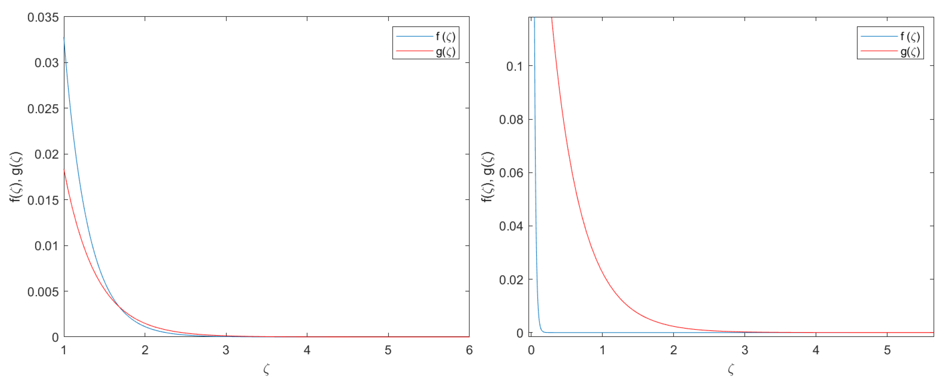
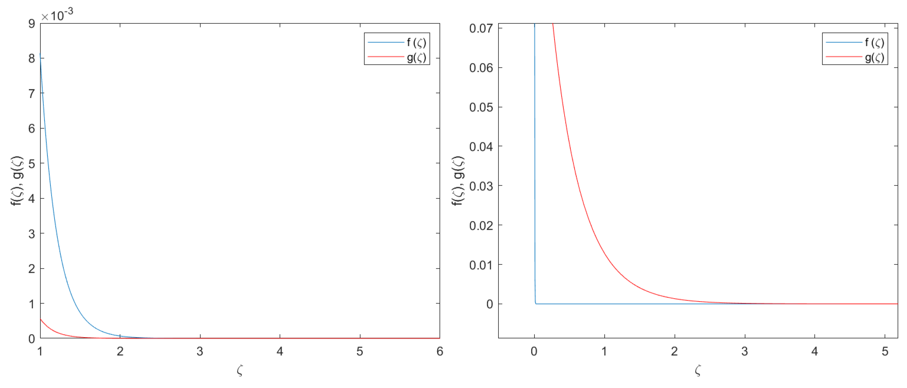
4. Numerical Validation

The idea in this section is to show that the analytical assessments done in previous sections are accurate to support asymptotic solutions to the Equation (10). To this end, a numerical exercise is provided to solve Equation (10) and then compared with the analytical solutions in expressions (44) and (48).

The numerical routine introduced in this section is provided for moderate values in the Reynolds number (to be representative of a porous medium) and in the assumption of:

$$A_1=1;0<M\ll 1,F=1,G=1.$$

(53)

The idea is to provide a validating exercise of the analytical assessments for certain values in the fluid parameters. The numerical exercise is not intended to provide solutions and to discuss them for different combinations in the parameters.

The following properties are of relevance:

• The numerical approach is done with the Matlab function bvp4c. This function is based on a Runge–Kutta implicit approach with interpolant extensions [38]. The bvp4c has a collocation method at the pseudo-boundary conditions given by $g(-\infty )=1$ and $g(\infty )=0$.
• The influence of the pseudo-boundary conditions and the collocation method shall be minimized. To this end, the integration domain is sufficiently large $(-1000,1000)$.
• To make the problem tractable in terms of computational efforts, the integration domain has been split into 100,000 nodes with an absolute accumulated error of ${10}^{-4}$. With this level of discretization, the problem has been simulated with standard computers and with reasonable computational lead times.

The results are provided in Figure 1 and Figure 2. The solutions are close for moderate values in the Reynolds number independently of the value of a. Note that the asymptotic convergence of travelling wave profiles to the numerical solution is given for $\zeta$ as sufficiently big. As described in each figure footprint, the criteria for asymptotic convergence between the analytical and numerical solutions is considered as the global distance $\le {10}^{-3}$. For this value and making numerical explorations, a dedicated value of ${\zeta }_{min}$ is found, such that for $\zeta \ge {\zeta }_{min}$, the global error is preserved.

Figure 1. Left: $c=1$, $Re=10$. Right: $c=1$, $Re=100$. Representation of solutions. Note that $g\left(\zeta \right)$ is the asymptotic solution as per expressions (44) and (48) and $f\left(\zeta \right)$ is the numerical resolution of Equation (36). For $Re=10$ (left), the global error between the analytical and numerical solution is ≤${10}^{-3}$ for $\zeta \ge 1.73$, while for $Re=100$ (right), the global error is ≤${10}^{-3}$ for $\zeta \ge 5.24$.

Figure 2. Left: $a=10$, $Re=10$. Right: $a=10$, $Re=100$. Representation of solutions, where $g\left(\zeta \right)$ is the asymptotic solution as per expressions (44) and (48) and $f\left(\zeta \right)$ is the numerical resolution of Equation (36). For $Re=10$ (left), the global error between the analytical and numerical solution is ≤${10}^{-3}$ for $\zeta \ge 1.13$, while for $Re=100$ (right), the global error is ≤${10}^{-3}$ for $\zeta \ge 2.34$.

5. Conclusions

The analysis discussed in this paper has provided results on the regularity of solutions to a fluid flow formulated with a degenerate diffusivity Eyring–Powell viscosity term and a Darcy–Forchheimer law in porous medium. Travelling wave profiles have been obtained and asymptotic solutions have been shown to hold based on the Geometric Perturbation Theory. The analytical assessments presented have been validated with a numerical exploration applicable for moderate values in the Reynolds number, i.e., in medium of high porosity. As a main finding to conclude upon, we highlight the existence of an exponential profile of the solution under an asymptotic approximation. This is not a trivial result and reflects that such an exponential profile holds as well for the case of degenerate diffusivity introduced. As a future research topic related with the presented analysis, the authors would like to bring attention to the introduction of further advanced numerical analyses in line with the references cited. In addition, other analytical techniques based in perturbation to solitons, $(G^{\prime }/G)$-expansion methods or maximal–minimal profiles may be explored to further precise the exponential solution found.

References

- Darcy, H. Les Fontaines Publiques de la Ville de Dijon; Dalmont: Paris, France, 1856. [Google Scholar]
- Forchheimer, P. Wasserbewegung durch Boden. Z. Vereines Dtsch. Ingeneieure 1901, 45, 1782–1788. [Google Scholar]
- Jaeger, C. Engineering Fluid Mechanics; Blackie and Son: Edinburgh, UK, 1956. [Google Scholar]
- Mohapatra, S.C.; Fonseca, R.B.; Soares, C.G. Comparison of Analytical and Numerical Simulations of Long Nonlinear Internal Solitary Waves in Shallow Water. J. Coast. Res. 2018, 34, 928–938. [Google Scholar] [CrossRef]
- Muskat, M. The Flow of Homogeneous Fluids through Porous Media; McGraw-Hill Book Company: New York, NY, USA, 1937. [Google Scholar]
- Ward, J.C. Flujo turbulento en medios porosos. Actas Div. Hidráulica Rev. ASCE 1964, 5, 1–12. [Google Scholar]
- Pal, D.; Mondal, H. Hydromagnetic convective diffusion of species in Darcy–Forchheimer porous medium with nonuniform heat source/sink and variable viscosity. Int. Commun. Heat Mass Transf. 2012, 39, 913–917. [Google Scholar] [CrossRef]
- Ganesh, N.A.; Hakeem, A.K.A.; Ganga, B. Darcy–Forchheimer flow of hydromagnetic nanofluid over a stretching/shrinking sheet in a thermally stratified porous medium with second order slip, viscous and ohmic dissipations effects. Ain Shams Eng. J. 2018, 9, 939–951. [Google Scholar] [CrossRef] [Green Version]
- Haq, R.U.; Soomro, F.A.; Mekkaouic, T.; Al-Mdallal, Q.M. MHD natural convection flow enclosure in a corrugated cavity filled with a porous medium. Int. J. Heat Mass Transf. 2018, 121, 1168–1178. [Google Scholar] [CrossRef]
- Hayat, T.; Muhammad, T.; Al-Mezal, S.; Liao, S.J. Darcy–Forchheimer flow with variable thermal conductivity and Cattaneo-Christov heat flux. Int. J. Numer. Methods Heat Fluid Flow 2016, 26, 2355–2369. [Google Scholar] [CrossRef]
- Abbas, W.; Megahed, A.M. Powell-Eyring fluid flow over a stratified sheet through porous medium with thermal radiation and viscous dissipation. AIMS Math. 2021, 6, 13464–13479. [Google Scholar] [CrossRef]
- Akbar, N.S.; Ebaid, A.; Khan, Z. Numerical analysis of magnetic field effects on Eyring–Powell fluid flow towards a stretching sheet. J. Magn. Magn. Mater. 2015, 382, 355–358. [Google Scholar] [CrossRef]
- Hina, S. MHD peristaltic transport of Eyring–Powell fluid with heat/mass transfer, wall properties and slip conditions. J. Magn. Magn. Mater. 2016, 404, 148–158. [Google Scholar] [CrossRef]
- Bhatti, M.; Abbas, T.; Rashidi, M.; Ali, M.; Yang, Z. Entropy generation on MHD Eyring–Powell nanofluid through a permeable stretching surface. Entropy 2016, 18, 224. [Google Scholar] [CrossRef] [Green Version]
- Ara, A.; Khan, N.A.; Khan, H.; Sultan, F. Radiation effect on boundary layer flow of an Eyring–Powell fluid over an exponentially shrinking sheet. Ain-Shams Eng. J. 2014, 5, 1337–1342. [Google Scholar] [CrossRef] [Green Version]
- Hayat, T.; Iqbal, Z.; Qasim, M.; Obaidat, S. Steady flow of an Eyring Powell fluid over a moving surface with convective boundary conditions. Int. J. Heat Mass Transf. 2012, 55, 1817–1822. [Google Scholar] [CrossRef]
- Hayat, T.; Awais, M.; Asghar, S. Radiative effects in a threedimensional flow of MHD Eyring–Powell fluid. J. Egypt Math. Soc. 2013, 21, 379–384. [Google Scholar] [CrossRef] [Green Version]
- Jalil, M.; Asghar, S.; Imran, S.M. Self similar solutions for the flow and heat transfer of Powell-Eyring fluid over a moving surface in parallel free stream. Int. J. Heat Mass Transf. 2013, 65, 73–79. [Google Scholar] [CrossRef]
- Khan, J.A.; Mustafa, M.; Hayat, T.; Farooq, M.A.; Alsaedi, A.; Liao, S.J. On model for three-dimensional flow of nanofluid: An application to solar energy. J. Mol. Liq. 2014, 194, 41–47. [Google Scholar] [CrossRef]
- Arshad, R.; Ellahi, R.; Sait, S.M. Role of hybrid nanoparticles in thermal performance of peristaltic flow of Eyring–Powell fluid model. J. Therm. Anal. Calorim. 2021, 143, 1021–1035. [Google Scholar]
- Díaz, J.L.; Rahman, S.; García-Haro, J.M. Heterogeneous Diffusion, Stability Analysis, and Solution Profiles for a MHD Darcy–Forchheimer Model. Mathematics 2022, 10, 20. [Google Scholar] [CrossRef]
- Murray, J. Mathematical Biology. In Biomathematics; Springer: Berlin/Heidelberg, Germany, 2013. [Google Scholar]
- Smolle, J. Shock Waves and Reactiondiffusion Equations; Springer Science Business Media: Berlin/Heidelberg, Germany, 2012; Volume 258. [Google Scholar]
- Champneys, A.; Hunt, G.; Thompson, J. Localization and Solitary Waves in Solid Mechanics; Advanced Series in Nonlinear Dynamics; World Scientific: Singapore, 1999. [Google Scholar]
- Kumar, R.N.; Jyothi, A.M.; Alhumade, H.; Gowda, R.J.P.; Alam, M.M.; Ahmad, I.; Gorji, M.R.; Prasannakumara, B.C. Impact of magnetic dipole on thermophoretic particle deposition in the flow of Maxwell fluid over a stretching sheet. J. Mol. Liq. 2021, 334, 116494. [Google Scholar] [CrossRef]
- Al-Mubaddel, F.S.; Farooq, U.; Al-Khaled, K.; Hussain, S.; Khan, S.U.; Aijaz, M.; Rahimi-Gorji, M.; Waqas, H. Double stratified analysis for bioconvection radiative flow of Sisko nanofluid with generalized heat/mass fluxes. Phys. Scr. 2021, 96, 5. [Google Scholar] [CrossRef]
- Dehghan, M.; Salehi, R. A meshfree weak-strong (MWS) form method for the unsteady magnetohydrodynamic (MHD) flow in pipe with arbitrary wall conductivity. Comput. Mech. 2013, 52, 1445–1462. [Google Scholar] [CrossRef]
- Dehghan, M.; Mirzaei, D. Meshless Local Petrov-Galerkin (MLPG) method for the unsteady magnetohydrodynamic (MHD) flow through pipe with arbitrary wall conductivity. Appl. Numer. Math. 2009, 59, 1043–1058. [Google Scholar] [CrossRef]
- Shakeri, F.; Dehghan, M. A finite volume spectral element method for solving magnetohydrodynamic (MHD) equations. Appl. Numer. Math. 2011, 61, 1–23. [Google Scholar] [CrossRef]
- Dehghan, M.; Abbaszadeh, M. Error analysis and numerical simulation of magnetohydrodynamics (MHD) equation based on the interpolating element free Galerkin (IEFG) method. Appl. Numer. Math. 2019, 137, 252–273. [Google Scholar] [CrossRef]
- Hosseinzadeh, H.; Dehghan, M.; Mirzaei, D. The boundary elements method for magneto-hydrodynamic (MHD) channel flows at high Hartmann. Appl. Math. Model. 2013, 37, 2337–2351. [Google Scholar] [CrossRef]
- Eldabe, N.; Hassan, A.; Mohamed, M.A. Effect of couple stresses on the MHD of a non-Newtonian unsteady flow between two parallel porous plates. Z. Fur Naturforschung A 2003, 58, 204–210. [Google Scholar] [CrossRef] [Green Version]
- De Pablo, A. Estudio de Una Ecuación de Reacción—Difusión. Ph.D. Thesis, Universidad Autónoma de Madrid, Madrid, Spain, 1989. [Google Scholar]
- De Pablo, A.; Vázquez, J.L. Travelling waves and finite propagation in a reactiondiffusion Equation. J. Differ. Equ. 1991, 93, 19–61. [Google Scholar] [CrossRef] [Green Version]
- Fenichel, N. Persistence and smoothness of invariant manifolds for flows. Indiana Univ. Math. J. 1971, 21, 193–226. [Google Scholar] [CrossRef]
- Akveld, M.E.; Hulshof, J. Travelling Wave Solutions of a Fourth-Order Semilinear Diffusion Equation. Appl. Math. Lett. 1998, 11, 115–120. [Google Scholar] [CrossRef] [Green Version]
- Jones, C.K.R.T. Geometric Singular Perturbation Theory in Dynamical Systems; Springer: Berlín, Germany, 1995. [Google Scholar]
- Enright, H.; Muir, P.H. A Runge-Kutta Type Boundary Value ODE Solver with Defect Control; Technical Reports; University of Toronto, Department of Computer Sciences: Toronto, ON, Canada, 1993; Volume 267, p. 93. [Google Scholar]
Publisher’s Note: MDPI stays neutral with regard to jurisdictional claims in published maps and institutional affiliations. |
© 2022 by the authors. Licensee MDPI, Basel, Switzerland. This article is an open access article distributed under the terms and conditions of the Creative Commons Attribution (CC BY) license (https://creativecommons.org/licenses/by/4.0/).