Abstract
The nonlocal Hirota–Maccari equation is considered when a parametric excitation is acting over the frequency of a generic mode. Using the well-known asymptotic perturbation (AP) method, two coupled equations for the amplitude and phase can be obtained. We discovered the existence of an infinite-period bifurcation when the parametric force increases its value. Moreover, symmetry considerations suggest performing a global analysis of the two couples, in such a way that we find an energy-like function and corroborate and verify the existence of this infinite period bifurcation.
1. Introduction
Resonances are recurrent topics in many physics problems. Usually, this means surprisingly large feedback when a little external perturbation is acting over the system. The undamped harmonic oscillator driven by an external force is a celebrated example, which is textbook material. If we study this simple linear oscillator, then one easily proves the existence of unbounded linearly increasing terms in the solution [1].
Nonlinear systems can also exhibit resonant behavior. We can consider many Hamiltonian chaotic systems in such a way that torus resonances are the reason for the origin of chaos, to cite only a few examples [2]. A similar picture can be observed when partial differential equations are investigated. Here, some results are known in simple linear cases, but in general, the study of resonances in complex nonlinear systems and the connected partial differential equations is always a difficult question [3,4,5,6,7,8].
We can think that a resonant perturbation can only excite a small number of modes in a nonlinear partial differential equation (NPDE). Usually, the nonlinearities mix different modes and the growth of one of them is forbidden by energy transfer to the others, specifically in conservative systems where the conservation laws are important constraints for the number and amplitude of active modes. Therefore, if the energy is transferred to the non-resonant modes and in cases when their growth is forbidden by nonlinear constraints, the role of the perturbation should be limited, and unbounded growth of the relevant quantities should be inhibited. Obviously, this is the common mechanism in many systems. However, other interesting behaviors can occur, and unexpected phenomena are possible even in a supposedly simple physically relevant model.
It can be demonstrated in this paper that an infinite period bifurcation can occur in the nonlocal Hirota–Maccari equation with two spatial dimensions and one temporal variable [9], if we consider a parametric resonance, when the external excitation frequency is nearly double that of a generic mode frequency.
Let us consider the following Hirota–Maccari equation
where is a suitable complex function and is a real function. The nonlocality is given by the real function ; its values depend on the complex function values all over the plane (x,y). The Hirota–Maccari equation substitutes the Kadomtsev–Petviashvili equation when we consider phenomena where the spatial scale in the x-direction is different from the spatial scale in the y-direction, and, in this case, the real part of the function ψ is the wave amplitude and the real function describes the nonlocal effects [10,11].
For x = y, we obtain the well-known one-dimensional Hirota equation [12] that describes the spread of the femto-second soliton pulse in the single-mode fibers.
Now, we introduce a parametric excitation that can induce a parametric resonance into Equation (1) and arrive to the following model system
where f is the parametric resonance amplitude, and the circular frequency of a given mode is
The external force is in parametric resonance () with the frequency of a generic mode.
In Section 2, using the asymptotic perturbation (AP) method [13], we build an approximate solution to Equations (3) and (4) and obtain two coupled equations for the solution amplitude and phase modulations.
In Section 3, we demonstrate the existence of an infinite-period bifurcation. If we increase the parametric strength from very small values, the solution oscillates with its almost natural frequency. However, when the excitation reaches a critical value, the solution frequency decreases further and further. We arrive to an infinite period or zero-frequency bifurcation.
As a consequence, if we carefully choose the initial conditions, then the approximate solution of Equations (3) and (4) becomes immobile, frozen and insensitive to the parametric excitation.
Finally, for higher values of the amplitude response, the frequency increases and we observe a modulated motion.
In Section 4, using symmetry considerations, a global analysis of the model system we obtained in Section 2 can be performed, utilizing an energy-like function, and the existence of an infinite period bifurcation can be validated.
In Section 5, the paper’s main findings are reviewed, and possible developments and directions for future work are discussed.
2. The Approximate Solution
The nonlocal Hirota–Maccari Equations (3) and (4) in resonance with a parametric excitation are investigated in this section; the forcing term f is scaled as , where ε is our small parameter, and we introduce the slow time
in order to consider larger time scales and find the amplitude modulation response.
Using the AP method [13], the approximate solution of Equations (3) and (4) can be written in the following form
and in Equation (7) is given by (6), where the boundary conditions are
The proximity of the excitation frequency Ω to the system frequency ω can be characterized through a detuning parameter σ,
where
Note that only a single leading mode is accounted for by the approximate solution. We assume that the system is excited near the natural frequency of a specific linear mode, and that mode is not involved in an in other resonances with any other mode. Following the AP method, the modes that are not directly excited by an external source or indirectly through an internal resonance will decay with time, if friction terms are present. Note that the variable change (6) implies that
We use the temporal rescaling (6) in order to find the asymptotic behavior of the solution, when the nonlinear amplitude can be modified by the nonlinear effects.
The elimination of the predominant linear part of Equations (3) and (4) is obtained by the assumed solution (7), and it allows us to calculate the amplitude modulation given by the parametric excitation.
After using solution (7) for the complete Equations (3) and (4), we obtain the linear equation
If we consider Equations (3) and (4) at the order, then we find that the function satisfies the nonlinear differential equation
The complex-valued function is characterized by its amplitude and phase
and we obtain at the model equations
where is a function of y and t, but for simplicity, we consider it as a constant. This model system (17, 18) describes the amplitude and phase evolution according to our starting assumptions. We observe that the validity of the approximate solution (7) should be expected to be kept under control on time-scale and on bounded intervals of the τ-variable. On the contrary, the approximate solution (7) loses its validity if we want to find solutions on larger intervals such that . In the next section, we will demonstrate the possibility of an infinite-period bifurcation for the nonlocal Hirota–Maccari equation.
3. A Reverse Infinite-Period Bifurcation
The fixed points of the model system (17, 18) are connected to periodic solutions of the starting system (3, 4), and we must consider the conditions . Note that the solution exists in the following cases
We can easily determine their possible stability, and through the Jacobian matrix, we obtain the equation
where, in the last equation, the minus sign is for the solution P1 (elliptic point) and the plus sign is for the solution P2 (saddle point).
From Equations (21a) and (21b), we can find the small oscillation frequency around the elliptic point
Using Equations (17) and (18), we arrive at the frequency-response equation
where now the equilibrium point amplitude is given by (19, 20) (Figure 1).
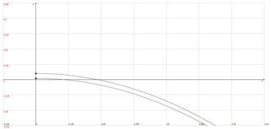
Figure 1.
Frequency (y = σ)-response (x = ρ) curve where K1 = 0.9, f = 0.02, φ = 0.03. The upper branch is the elliptic point, the lower branch corresponds to the saddle point.
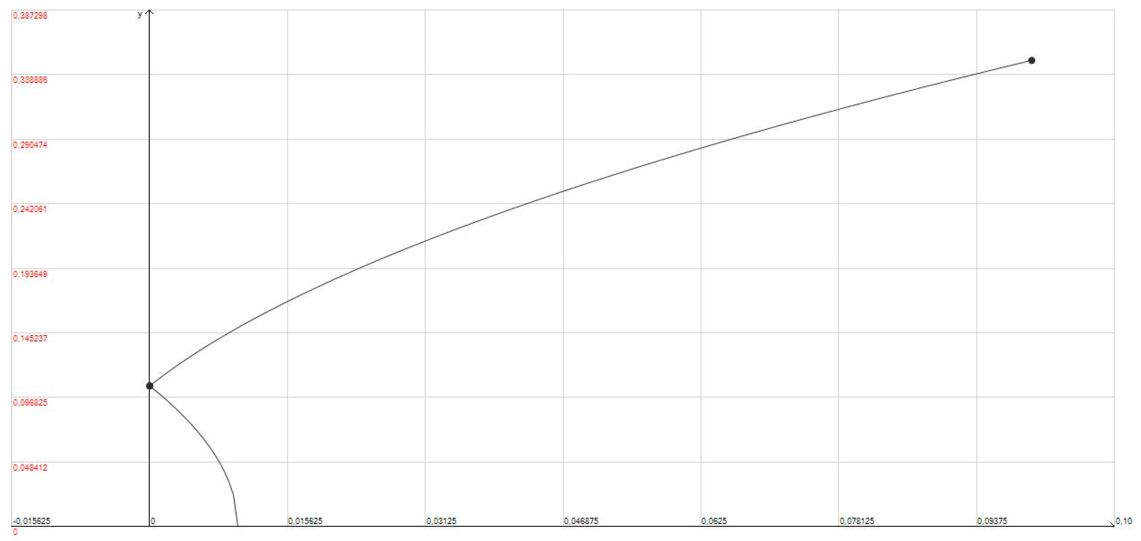
Subsequently, we show the response-parametric excitation curve (Figure 2). For the elliptic point, the response increases with the parametric excitation.
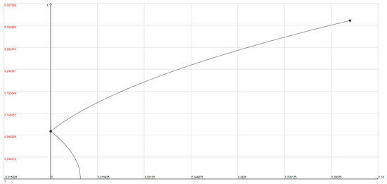
Figure 2.
Response (y = ρ)-parametric excitation (x = f) curve where K1 = 0.9, σ = 0.02, φ = 0.03. The upper branch is the elliptic point, the lower branch corresponds to the saddle point.
We show that an infinite-period bifurcation occurs near the elliptic point, but it is more convenient if we consider increasing parametric excitation values.
We observe the following situation (, the excitation frequency Ω is slightly smaller than the double of ω, near the equilibrium point P1):
(i) When f = 0, there is no parametric excitation and the wave amplitude is constant;
(ii) When the excitation is weak, there are no equilibrium points because of (3.1) and the wave amplitude begins to oscillate with an amplitude increasing with the excitation amplitude f and the frequency
(iii) If the external excitation increases and reaches the critical value
the oscillation frequency decreases and the wave seems to collapse, but actually it begins a very slow oscillation, meaning metaphorically that it dies and is born again, with a large period, and an infinite-period bifurcation occurs when (Figure 3).

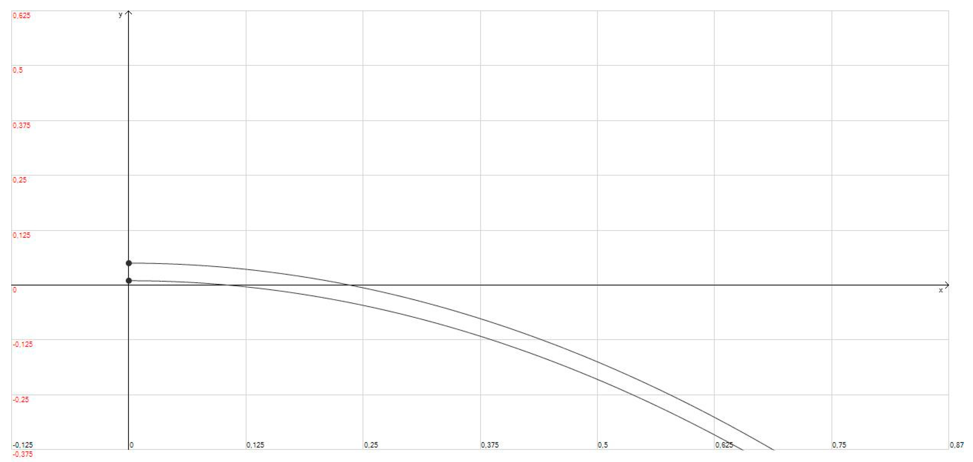
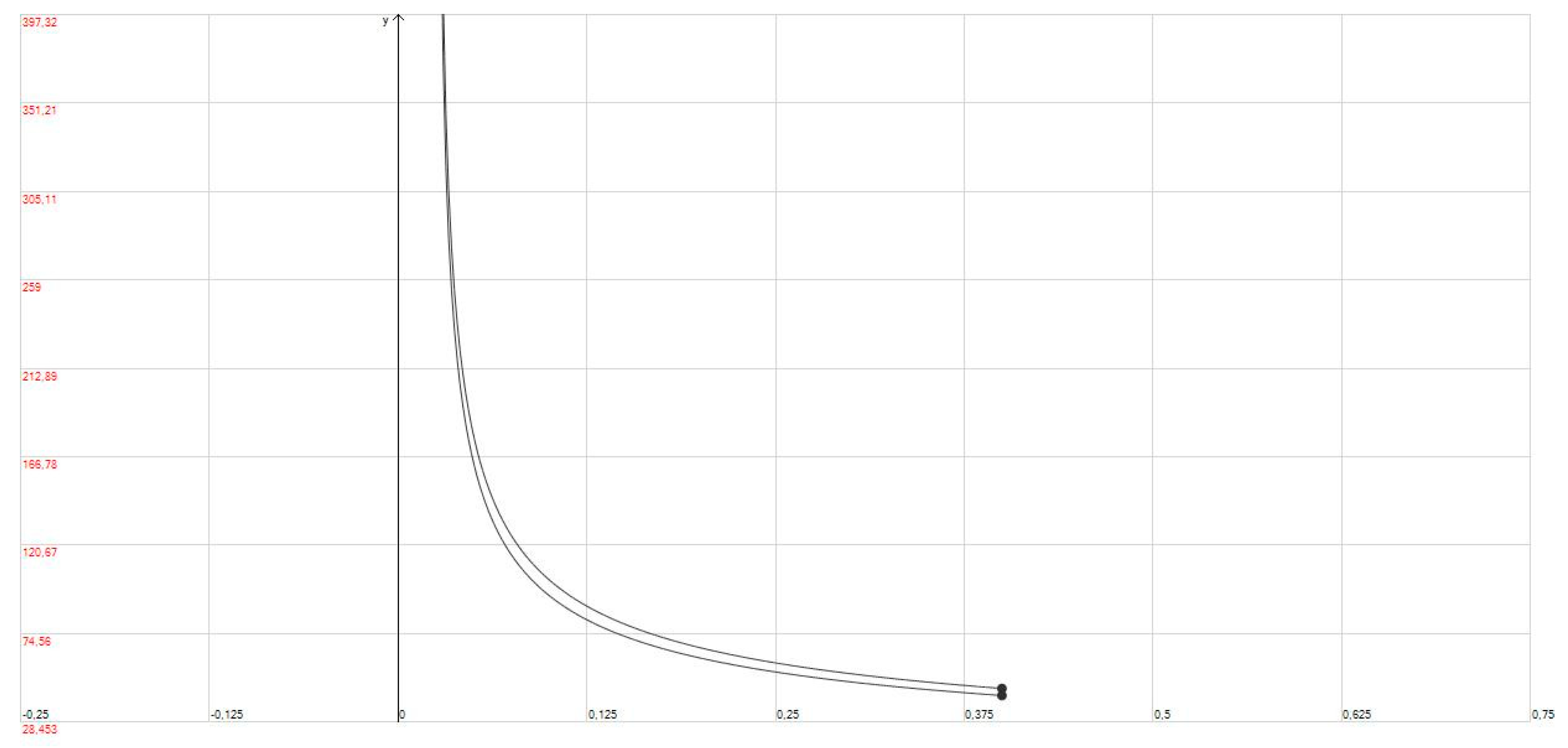
Figure 3.
Infinite-period bifurcation. We show the period T = y-axis and the parametric excitation f = x-axis, when fC is 0.025 or fC = 0.023.
We can estimate the oscillation period T assuming in our calculations
(iv) If the initial condition for the wave amplitude is carefully tuned, that is, it corresponds to P1, then the wave amplitude seems immobile, frozen and insensitive to the external excitation with no oscillation;
(v) Suddenly, beyond the critical value (25) and for higher response amplitude values, a slow oscillation appears with the frequency
4. Global Analysis of the Model System
A global analysis of the model system (17, 18) can be performed. Considering the model system (17, 18), we obtain an energy-like function
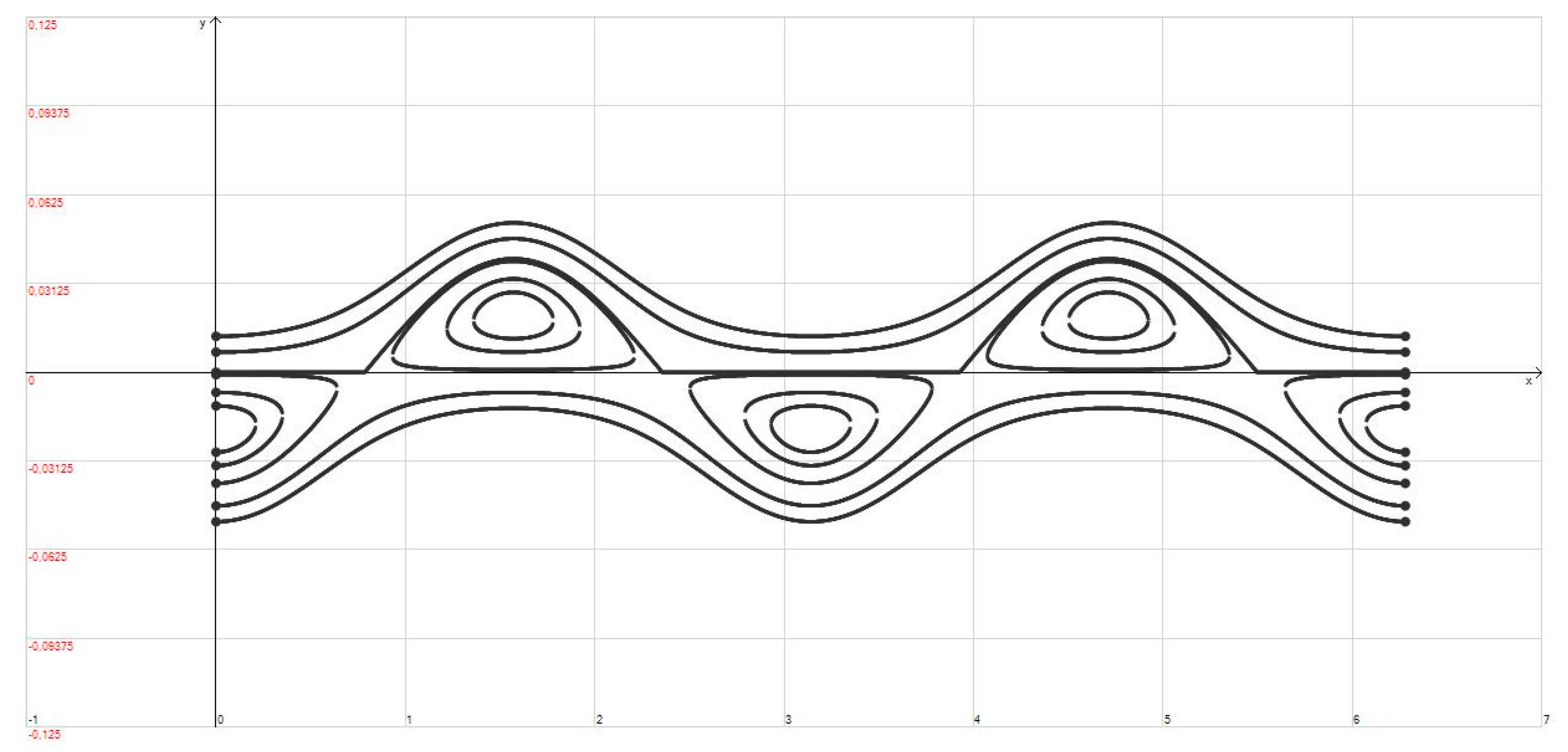
We can easily conclude that every function in the form , with real numbers, can be used as an energy function. We can take = 1 so that the elliptic point P1 corresponds to a minimum. In Figure 4, we show the level curves for the energy function (28) near the equilibrium point (19), and we can easily observe that the infinite-period bifurcation is connected to the “bottleneck” we can see in the same figure. The bottleneck is, when in the closed curves in Figure 4, the ρ-value (y-axis) is constant and ϑ (x-axis) is varying.
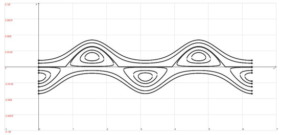
Figure 4.
Level curves in the plane x = ϑ and y = ρ. (K1 = 0.6, f = 0.02, σ = φ). Obviously, only positive values for ρ are acceptable. From the upper side, we show level curves for energy E = 0.0002, 0.0001 and 0 and we can observe a modulated motion. Subsequently, we obtain closed curves for E = −0.00001, −0.00007, −0.0001.
The fixed point (19) downshifts the solution motion near it, and a lower frequency is born.
5. Conclusions
The nonlocal Hirota–Maccari equation with an external periodic force in parametric resonance with a generic mode has been investigated. An approximate solution with the AP perturbation method, previously used for other nonlinear partial differential equations, was suggested and analyzed qualitatively in the vicinity of critical point fC. Two coupled nonlinear equations describe the temporal evolution for the solution amplitude and phase. Frequency-response curves are shown and the existence of an infinite-period bifurcation (when the parametric excitation increases in magnitude) can be demonstrated.
Looking at Equations (19), (22) and (26), it is possible to discern certain analogies with the Hopf–Landau theory of turbulence [1,14].
This perturbation method could be applied to important resonances for other nonlinear partial differential equations in plasma physics and/or nonlinear optics.
Funding
This research received no external funding.
Data Availability Statement
Data sharing not applicable to this article as no datasets were generated or analyzed during the current study.
Conflicts of Interest
The author declares that there are no conflicts of interest.
References
- Fossen, T.; Nijmeijer, H. (Eds.) Parametric Resonance in Dynamical Systems; Springer: New York, NY, USA, 2011. [Google Scholar]
- Kim, S.; Mackay, R.S.; Guckenheimer, J. Resonance regions for families of torus maps. Nonlinearity 1989, 2, 391–404. [Google Scholar] [CrossRef]
- Sahoo, S.K.; Das, H.C.; Panda, C.L. An overview of transverse vibration of axially travelling string. In Recent Trends in Applied Mathematics; Mishra, S.R., Dhamala, T.N., Makinde, O.D., Eds.; Springer: New York, NY, USA, 2021; pp. 427–446. [Google Scholar]
- Jackson, R.K.; Weinstein, M.I. Geometric Analysis of Bifurcation and Symmetry Breaking in a Gross–Pitaevskii Equation. J. Stat. Phys. 2004, 116, 881–905. [Google Scholar] [CrossRef] [Green Version]
- Susanto, H.; Cuevas, J.; Kruger, P. Josephson tunnelling of dark solitons in a double-well potential. J. Phys. B At. Mol. Opt. Phys. 2011, 44, 059003. [Google Scholar] [CrossRef] [Green Version]
- Susanto, H.; Cuevas, J. Josephson Tunneling of Excited States in a Double-Well Potential, in Sponaneous Symmetry Breaking. In Self-Trapping, and Josephson Oscillations; Springer: Berlin/Heidelberg, Germany, 2012; pp. 583–599. [Google Scholar]
- Marangell, R.; Jones, R.T.; Susanto, H. Localized standing waves in inhomogenous Schrödinger equations. Nonlinearity 2010, 23, 2059. [Google Scholar] [CrossRef]
- Marangell, R.; Jones, R.T.; Susanto, H. Instability of standing waves for nonlinear Schrödinger-type equations. J. Differ. Equ. 2012, 253, 1191–1205. [Google Scholar] [CrossRef] [Green Version]
- Maccari, A. A generalized Hirota equation in 2+1 dimensions. J. Math. Phys. 1998, 39, 6547–6551. [Google Scholar] [CrossRef]
- Demiray, S.T.; Pandir, Y.; Bulut, H. All exact travelling wave solutions of Hirota equation and Hirota–Maccari system. Optik 2016, 127, 1848–1859. [Google Scholar] [CrossRef]
- Xia, P.; Zhang, Y.; Zhang, H.; Zhuang, Y. Some novel dynamical behavior of localized solitary waves for the Hirota-Maccari system. Nonlinear Dyn. 2022, 108, 533–541. [Google Scholar] [CrossRef]
- Hirota, R. Exact envelope-soliton solutions of a nonlinear wave equation. J. Math. Phys. 1973, 14, 805–809. [Google Scholar] [CrossRef]
- Maccari, A. Coherent solutions for the fundamental resonance of the Boussinesq equation. Chaos Solitons Fractals 2013, 54, 57–64. [Google Scholar] [CrossRef]
- Gluzman, S.; Karpeev, D. Perturbative expansions and critical phenomenain random structured media. In Modern Problems in Applied Analysis; Drygaś, P., Rogosin, S., Eds.; Birkhauser: Basel, Switzerland, 2018; pp. 117–134. [Google Scholar]
Publisher’s Note: MDPI stays neutral with regard to jurisdictional claims in published maps and institutional affiliations. |
© 2022 by the author. Licensee MDPI, Basel, Switzerland. This article is an open access article distributed under the terms and conditions of the Creative Commons Attribution (CC BY) license (https://creativecommons.org/licenses/by/4.0/).