
A Scaled Dai–Yuan Projection-Based Conjugate Gradient Method for Solving Monotone Equations with Applications

 , ,
, , 
Abstract
1. Introduction
2. A Scaled Dai–Yuan CG Methods
2.1. Scaling Parameter Based on the Quasi-Newton Approach
2.2. Scaling Parameter Based on Barzilai–Borwein Approach
| Algorithm 1: The spectral DY CG projection-based algorithm (SDYCG) |
Step 0 Initialize: , , , , , and . Set and . Step 1 If , stop; otherwise, go to Step 2. , and . Step 3 Set and determine satisfying
Step 4 If and stop; otherwise
where
Step 5 Set and then go to Step 1. |
3. Global Convergence
- A1 The solution set is non-empty.
- A2 The function F is Lipschitz continuous for , i.e., for
- A3 The function F satisfies (2).
- Additionally, from the monotonicity assumption on F, we have
4. Numerical Experiment and Applications
4.1. Application to the Monotone Nonlinear Equations
- , and
- , ,
- and
- for and
- , and .
- for ,
- , and .
- , for , and .
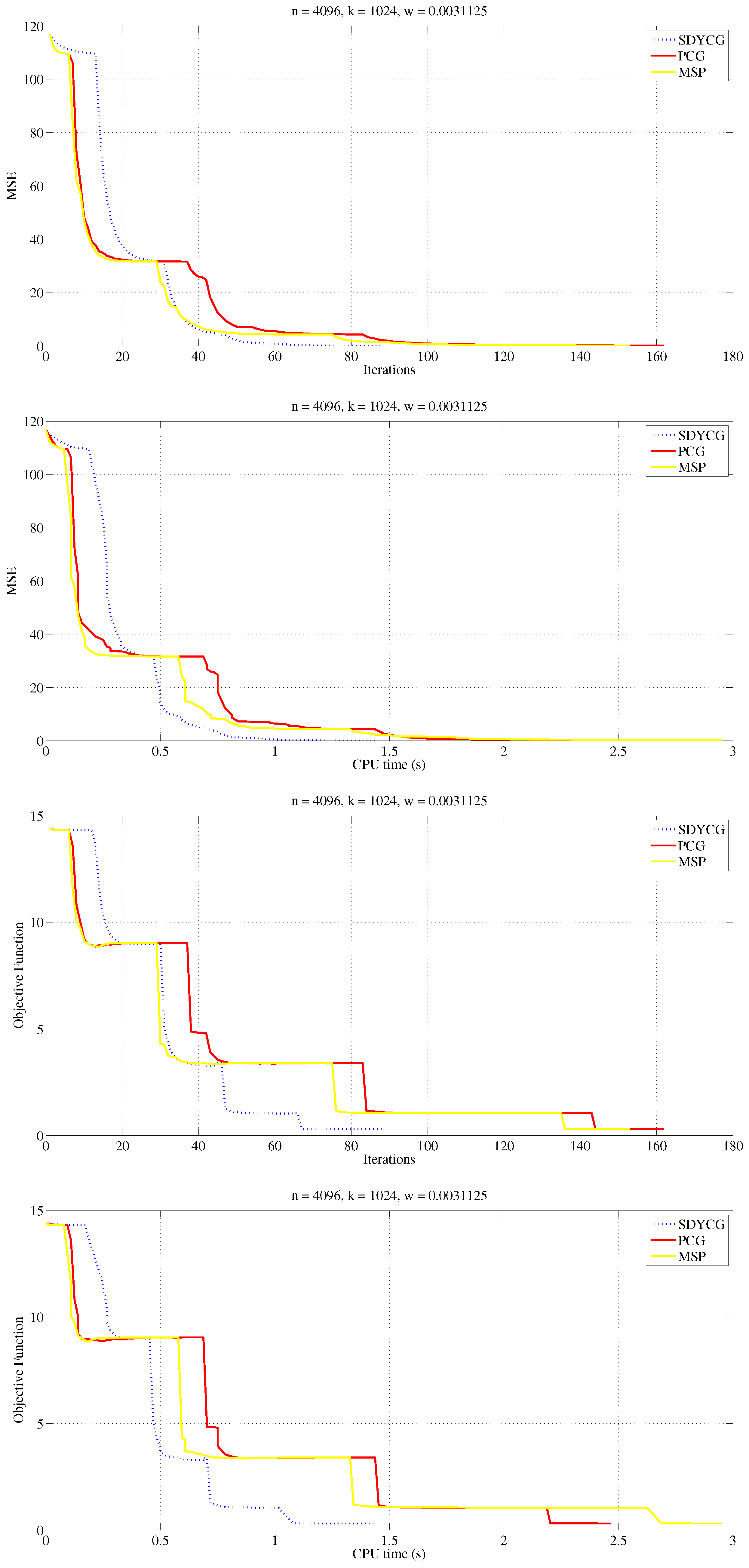
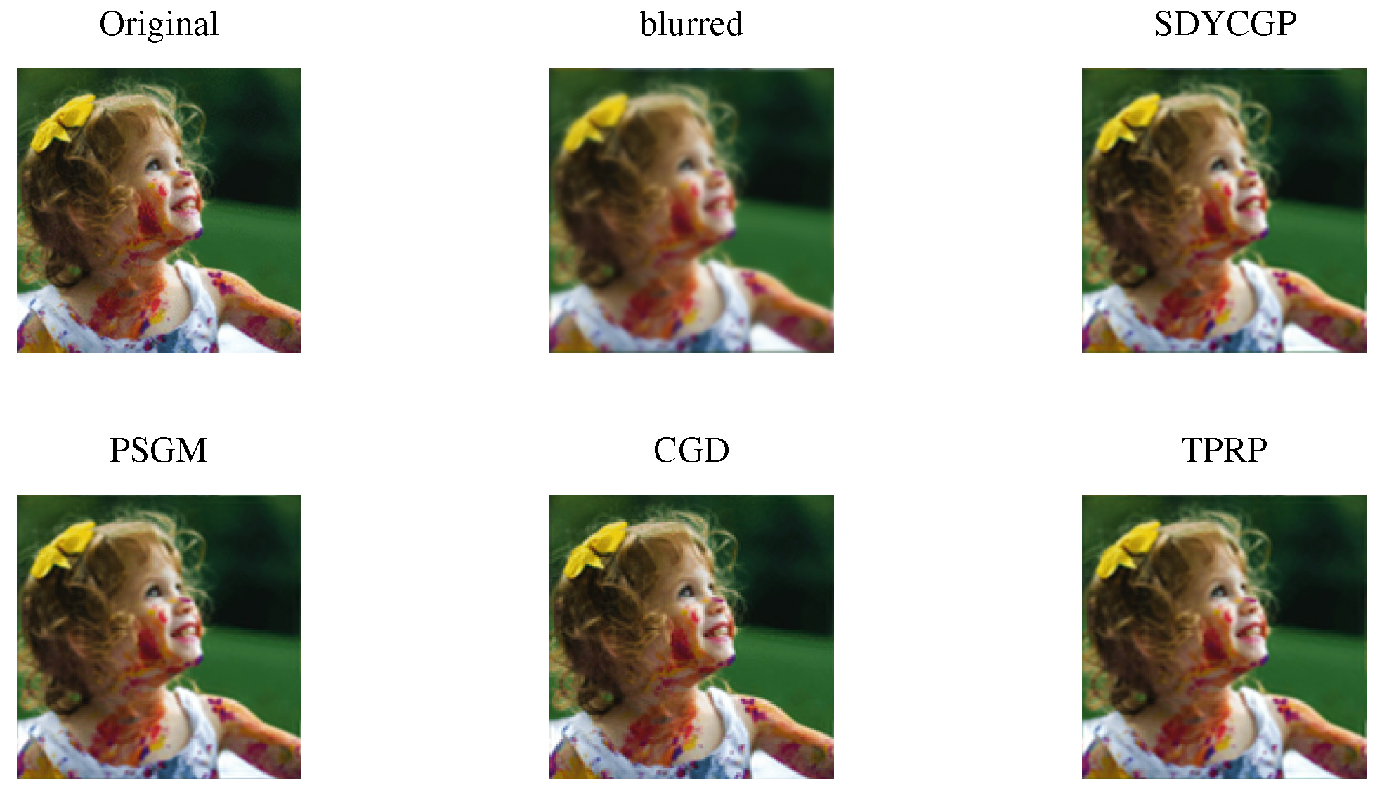
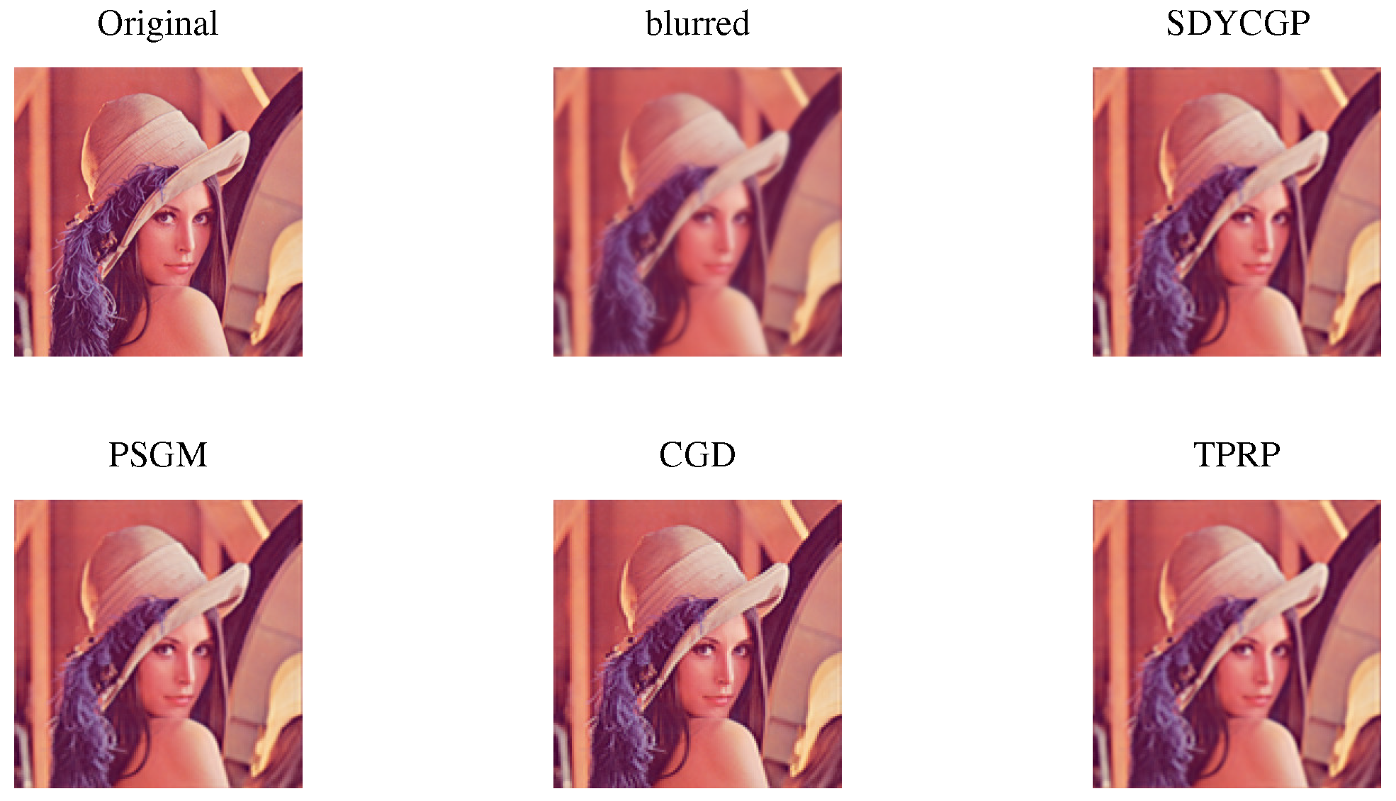
4.2. Application in Signal Recovery
5. Conclusions
Author Contributions
Funding
Institutional Review Board Statement
Informed Consent Statement
Data Availability Statement
Conflicts of Interest
References
- Dai, Z.; Zhou, H.; Wen, F.; He, S. Efficient predictability of stock return volatility: The role of stock market implied volatility. N. Am. J. Econ. Finance 2020, 52, 101174. [Google Scholar] [CrossRef]
- Figueiredo, M.A.; Nowak, R.D.; Wright, S.J. Gradient projection for sparse reconstruction, application to compressed sensing and other inverse problems. IEEE J. Sel. Top. Signal Process. 2007, 1, 586–597. [Google Scholar] [CrossRef]
- Iusem, A.N.; Solodov, M.V. Newton-type methods with generalized distances for constrained optimization. Optimization 1997, 41, 257–278. [Google Scholar] [CrossRef]
- Zhao, Y.B.; Li, D.H. Monotonicity of fixed point and normal mapping associated with variational inequality and its application. SIAM J. Optim. 2001, 4, 962–973. [Google Scholar] [CrossRef]
- Ortega, J.M.; Rheinboldt, W.C. Iterative Solution of Nonlinear Equations in Several Variables; Academic Press: Cambridge, MA, USA, 1970. [Google Scholar]
- Zhou, G.; Toh, K.C. Superlinear convergence of a Newton-type algorithm for monotone equations. J. Optimiz. Theory App. 2005, 125, 205–221. [Google Scholar] [CrossRef]
- Zhou, W.J.; Li, D.H. A globally convergent BFGS method for nonlinear monotone equations without any merit functions. Math. Comput. 2008, 77, 2231–2240. [Google Scholar] [CrossRef]
- Sabi’u, J.; Shah, A.; Waziri, M.Y.; Ahmed, K. Modified Hager-Zhang conjugate gradient methods via singular value analysis for solving monotone nonlinear equations with convex constraint. Int. J. Comput. Methods 2020, 18, 2050043. [Google Scholar] [CrossRef]
- Sabi’u, J.; Shah, A.; Waziri, M.Y. A modified Hager-Zhang conjugate gradient method with optimal choices for solving monotone nonlinear equations. Int. J. Comput. Math. 2021, 99, 1–23. [Google Scholar] [CrossRef]
- Sabi’u, J.; Shah, A. An efficient three-term conjugate gradient-type algorithm for monotone nonlinear equations. RAIRO-Oper Res. 2021, 55, 1113. [Google Scholar] [CrossRef]
- Waziri, M.Y.; Ahmed, K.; Sabi’u, J.; Halilu, A.S. Enhanced Dai–Liao conjugate gradient methods for systems of monotone nonlinear equations. SeMA J. 2021, 78, 15–51. [Google Scholar] [CrossRef]
- Abubakar, A.B.; Sabi’u, J.; Kumam, P.; Shah, A. Solving nonlinear monotone operator equations via modified sr1 update. J. Appl. Math. Comput. 2021, 67, 1–31. [Google Scholar] [CrossRef]
- Waziri, M.Y.; Hungu, K.A.; Sabi’u, J. Descent Perry conjugate gradient methods for systems of monotone nonlinear equations. Numer. Algorithms 2020, 85, 763–785. [Google Scholar] [CrossRef]
- Waziri, M.Y.; Ahmed, K.; Sabi’u, J. A Dai–Liao conjugate gradient method via modified secant equation for system of nonlinear equations. Arab. J. Math. 2020, 9, 443–457. [Google Scholar] [CrossRef]
- Sabi’u, J.; Shah, A.; Waziri, M.Y. Two optimal Hager-Zhang conjugate gradient methods for solving monotone nonlinear equations. Appl. Numer. Math. 2020, 153, 217–233. [Google Scholar] [CrossRef]
- Dai, Y.H.; Yuan, Y. A nonlinear conjugate gradient method with a strong global convergence property. SIAM J. Optim. 1999, 10, 177–182. [Google Scholar] [CrossRef]
- Waziri, M.Y.; Ahmed, K. Two Descent Dai–Yuan Conjugate Gradient Methods for Systems of Monotone Nonlinear Equations. J. Sci. Comput. 2022, 90, 1–53. [Google Scholar] [CrossRef]
- Kambheera, A.; Ibrahim, A.H.; Muhammad, A.B.; Abubakar, A.B.; Hassan, B.A. Modified Dai–Yuan Conjugate Gradient Method with Sufficient Descent Property for Nonlinear Equations. Thai J. Math. 2022, 145–167. Available online: http://thaijmath.in.cmu.ac.th/index.php/thaijmath/article/viewFile/6026/354355047 (accessed on 6 June 2022).
- Aji, S.; Kumam, P.; Awwal, A.M.; Yahaya, M.M.; Sitthithakerngkiet, K. An efficient DY-type spectral conjugate gradient method for system of nonlinear monotone equations with application in signal recovery. AIMS Math. 2021, 6, 8078–8106. [Google Scholar] [CrossRef]
- Abdullahi, H.; Awasthi, A.K.; Waziri, M.Y.; Halilu, A.S. Descent three-term DY-type conjugate gradient methods for constrained monotone equations with application. Comput. Appl. Math. 2022, 41, 1–28. [Google Scholar] [CrossRef]
- Sabi’u, J.; Aremu, K.O.; Althobaiti, A.; Shah, A. Scaled three-term conjugate gradient methods for solving monotone equations with application. Symmetry 2022, 14, 936. [Google Scholar] [CrossRef]
- Barzilai, J.; Borwein, J.M. Two-point step size gradient methods. IMA J. Numer. Anal. 1988, 8, 141–148. [Google Scholar] [CrossRef]
- Zheng, L.; Yang, L.; Liang, Y. A modified spectral gradient projection method for solving non-linear monotone equations with convex constraints and its application. IEEE Access 2020, 8, 92677–92686. [Google Scholar] [CrossRef]
- Amini, K.; Faramarzi, P.; Bahrami, S. A spectral conjugate gradient projection algorithm to solve the large-scale system of monotone nonlinear equations with application to compressed sensing. Int. J. Comp. Math. 2022, 1–18. [Google Scholar] [CrossRef]
- La Cruz, W.; Martinez, J.; Raydan, M. Spectral residual method without gradient information for solving large-scale nonlinear systems of equations. Math. Comput. 2006, 75, 1429–1448. [Google Scholar] [CrossRef]
- Halilu, A.S.; Majumder, A.; Waziri, M.Y.; Ahmed, K. Signal recovery with convex constrained nonlinear monotone equations through conjugate gradient hybrid approach. Math Comput. Simul. 2021, 187, 520–539. [Google Scholar] [CrossRef]
- Liu, J.; Duan, Y. Two spectral gradient projection methods for constrained equations and their linear convergence rate. J. Inequal. Appl. 2015, 2015, 1–13. [Google Scholar] [CrossRef]
- Dolan, E.D.; Moré, J.J. Benchmarking optimization software with performance profiles. Math. Program. 2002, 91, 201–213. [Google Scholar] [CrossRef]
- Hale, E.T.; Yin, W.; Zhang, Y. A fixed-point continuation method for l1 regularized minimization with applications to compressed sensing. SIAM J. Optim. 2008, 19, 1107–1130. [Google Scholar] [CrossRef]
- Beck, A.; Teboulle, M. A fast iterative shrinkage-thresholding algorithm for linear inverse problems. SIAM J. Imag. Sci. 2009, 2, 183–202. [Google Scholar] [CrossRef]
- Van den Berg, E.; Friedlander, M.P. Probing the pareto frontier for basis pursuit solutions. SIAM J. Sci. Comput. 2008, 31, 890–912. [Google Scholar] [CrossRef]
- Xiao, Y.H.; Wang, Q.Y.; Hu, Q.J. Non-smooth equations based method for l1-norm problems with applications to compressed sensing. Nonlinear Anal. TMA 2011, 74, 3570–3577. [Google Scholar] [CrossRef]
- Pang, J.S. Inexact Newton methods for the nonlinear complementarity problem. Math. Program. 1986, 36, 54–71. [Google Scholar] [CrossRef]
- Awwal, A.M.; Kumam, P.; Mohammad, H.; Watthayu, W.; Abubakar, A.B. A Perry-type derivative-free algorithm for solving nonlinear system of equations and minimizing l1 regularized problem. Optimization 2021, 70, 1231–1259. [Google Scholar] [CrossRef]
- Xiao, Y.H.; Zhu, H. A conjugate gradient method to solve convex constrained monotone equations with applications in compressive sensing. J. Math. Anal. Appl. 2013, 405, 310–319. [Google Scholar] [CrossRef]
- Ibrahim, A.H.; Deepho, J.; Abubakar, A.B.; Adamu, A. A three-term Polak-Ribière-Polyak derivative-free method and its application to image restoration. Sci. Afr. 2021, 13, e00880. [Google Scholar] [CrossRef]
- Liu, J.K.; Lia, S.J. A projection method for convex constrained monotone nonlinear equations with applications. Comput. Math. Appl. 2015, 70, 2442–2453. [Google Scholar] [CrossRef]
- Abubakar, A.B.; Kumam, P.; Mohammad, H.; Awwal, A.M. A Barzilai-Borwein gradient projection method for sparse signal and blurred image restoration. J. Franklin Inst. 2020, 357, 7266–7285. [Google Scholar] [CrossRef]


| Problem 1 | SDYCG(1) | SDYCG(2) | MSGP | DFSP | |||||||||||||
|---|---|---|---|---|---|---|---|---|---|---|---|---|---|---|---|---|---|
| DIMENSION | INITIAL POINT | ITER | FVAL | TIME | NORM | ITER | FVAL | TIME | NORM | ITER | FVAL | TIME | NORM | ITER | FVAL | TIME | NORM |
| 500 | 2 | 27 | 0.178052 | 0 | 2 | 27 | 0.030794 | 0 | 121 | 1538 | 0.102812 | 9.3 | 7 | 73 | 0.051887 | 0 | |
| 2 | 27 | 0.007911 | 0 | 2 | 27 | 0.010431 | 0 | 91 | 1173 | 0.075893 | 8.58 | 4 | 45 | 0.025909 | 0 | ||
| 2 | 27 | 0.004025 | 0 | 2 | 27 | 0.004284 | 0 | 95 | 1200 | 0.146293 | 8.29 | 6 | 69 | 0.013521 | 0 | ||
| 3 | 40 | 0.008521 | 0 | 3 | 40 | 0.008234 | 0 | Fail | Fail | Fail | Fail | 5 | 57 | 0.011795 | 0 | ||
| 2 | 27 | 0.006885 | 0 | 2 | 27 | 0.006878 | 0 | Fail | Fail | Fail | Fail | 5 | 56 | 0.011774 | 0 | ||
| 2 | 27 | 0.005948 | 0 | 2 | 27 | 0.008259 | 0 | 57 | 725 | 0.042269 | 8.33 | 6 | 72 | 0.014265 | 0 | ||
| 2 | 27 | 0.004092 | 0 | 2 | 27 | 0.006461 | 0 | Fail | Fail | Fail | Fail | 5 | 56 | 0.01217 | 0 | ||
| 5 | 66 | 0.009501 | 0 | 5 | 66 | 0.013534 | 0 | 2 | 18 | 0.004343 | 0 | 2 | 17 | 0.07065 | 0 | ||
| 1000 | 2 | 27 | 0.004634 | 0 | 2 | 27 | 0.008994 | 0 | 134 | 1706 | 0.322519 | 9.92 | 8 | 84 | 0.022746 | 0 | |
| 2 | 27 | 0.009655 | 0 | 2 | 27 | 0.009192 | 0 | 91 | 1173 | 0.225743 | 8.59 | 4 | 45 | 0.012467 | 0 | ||
| 2 | 27 | 0.008619 | 0 | 2 | 27 | 0.009266 | 0 | 89 | 1122 | 0.212044 | 7.94 | 9 | 78 | 0.019796 | 0 | ||
| 3 | 40 | 0.00906 | 0 | 3 | 40 | 0.011755 | 0 | Fail | Fail | Fail | Fail | 5 | 56 | 0.01559 | 0 | ||
| 2 | 27 | 0.006779 | 0 | 2 | 27 | 0.008895 | 0 | Fail | Fail | Fail | Fail | 5 | 56 | 0.015161 | 0 | ||
| 2 | 27 | 0.004795 | 0 | 2 | 27 | 0.007495 | 0 | 57 | 725 | 0.138729 | 7.84 | 6 | 72 | 0.019059 | 0 | ||
| 2 | 27 | 0.006632 | 0 | 2 | 27 | 0.009641 | 0 | Fail | Fail | Fail | Fail | 5 | 56 | 0.015644 | 0 | ||
| 5 | 66 | 0.017444 | 0 | 5 | 66 | 0.017055 | 0 | 2 | 18 | 0.004908 | 0 | 2 | 17 | 0.006929 | 0 | ||
| 10,000 | 2 | 27 | 0.047267 | 0 | 2 | 27 | 0.041266 | 0 | 104 | 1311 | 1.560793 | 9.44 | 8 | 65 | 0.116677 | 0 | |
| 2 | 27 | 0.03194 | 0 | 2 | 27 | 0.039564 | 0 | 91 | 1173 | 1.997119 | 8.6 | 4 | 45 | 0.080051 | 0 | ||
| 2 | 27 | 0.031136 | 0 | 2 | 27 | 0.041833 | 0 | 98 | 1230 | 2.601348 | 9.08 | 9 | 68 | 0.123208 | 0 | ||
| 3 | 40 | 0.057081 | 0 | 3 | 40 | 0.056858 | 0 | Fail | Fail | Fail | Fail | 5 | 56 | 0.09662 | 0 | ||
| 2 | 27 | 0.035342 | 0 | 2 | 27 | 0.040675 | 0 | Fail | Fail | Fail | Fail | 5 | 56 | 0.103659 | 0 | ||
| 2 | 27 | 0.027089 | 0 | 2 | 27 | 0.038279 | 0 | 56 | 712 | 1.482753 | 9.8 | 6 | 72 | 0.126239 | 0 | ||
| 2 | 27 | 0.041587 | 0 | 2 | 27 | 0.04066 | 0 | Fail | Fail | Fail | Fail | 5 | 56 | 0.102553 | 0 | ||
| 5 | 66 | 0.089053 | 0 | 5 | 66 | 0.111986 | 0 | 2 | 18 | 0.042366 | 0 | 3 | 30 | 0.054729 | 0 | ||
| 50,000 | 2 | 27 | 0.119851 | 0 | 2 | 27 | 0.192334 | 0 | 103 | 1293 | 10.94405 | 9.7 | 10 | 89 | 0.690911 | 0 | |
| 2 | 27 | 0.158001 | 0 | 2 | 27 | 0.181709 | 0 | 91 | 1173 | 8.038891 | 8.6 | 4 | 45 | 0.329212 | 0 | ||
| 2 | 27 | 0.1872 | 0 | 2 | 27 | 0.195489 | 0 | Fail | Fail | Fail | Fail | 7 | 71 | 0.520311 | 0 | ||
| 3 | 40 | 0.170595 | 0 | 3 | 40 | 0.294915 | 0 | Fail | Fail | Fail | Fail | 5 | 56 | 0.425746 | 0 | ||
| 2 | 27 | 0.182155 | 0 | 2 | 27 | 0.19715 | 0 | Fail | Fail | Fail | Fail | 5 | 56 | 0.418211 | 0 | ||
| 2 | 27 | 0.118753 | 0 | 2 | 27 | 0.188444 | 0 | 56 | 712 | 4.008244 | 9.74 | 6 | 72 | 0.527691 | 0 | ||
| 2 | 27 | 0.191926 | 0 | 2 | 27 | 0.199747 | 0 | Fail | Fail | Fail | Fail | 5 | 56 | 0.421186 | 0 | ||
| 5 | 66 | 0.363679 | 0 | 5 | 66 | 0.467007 | 0 | 2 | 18 | 0.142288 | 0 | 3 | 30 | 0.223121 | 0 | ||
| 100,000 | 2 | 27 | 0.447002 | 0 | 2 | 27 | 0.423225 | 0 | 116 | 1456 | 17.30029 | 9.17 | 9 | 67 | 1.114614 | 0 | |
| 2 | 27 | 0.282127 | 0 | 2 | 27 | 0.398508 | 0 | 91 | 1173 | 13.14327 | 8.6 | 4 | 45 | 0.864917 | 0 | ||
| 2 | 27 | 0.438826 | 0 | 2 | 27 | 0.439531 | 0 | Fail | Fail | Fail | Fail | 11 | 124 | 1.896561 | 0 | ||
| 3 | 40 | 0.459044 | 0 | 3 | 40 | 0.630171 | 0 | Fail | Fail | Fail | Fail | 5 | 56 | 0.951345 | 0 | ||
| 2 | 27 | 0.457132 | 0 | 2 | 27 | 0.441214 | 0 | Fail | Fail | Fail | Fail | 5 | 56 | 1.073445 | 0 | ||
| 2 | 27 | 0.387432 | 0 | 2 | 27 | 0.398113 | 0 | 56 | 712 | 8.451864 | 9.73 | 6 | 72 | 1.197623 | 0 | ||
| 2 | 27 | 0.512523 | 0 | 2 | 27 | 0.424911 | 0 | Fail | Fail | Fail | Fail | 5 | 56 | 0.959261 | 0 | ||
| 5 | 66 | 0.76242 | 0 | 5 | 66 | 0.992397 | 0 | 2 | 18 | 0.266698 | 0 | 3 | 30 | 0.545118 | 0 | ||
| Problem 2 | SDYCG(1) | SDYCG(2) | MSGP | DFSP | |||||||||||||
|---|---|---|---|---|---|---|---|---|---|---|---|---|---|---|---|---|---|
| DIMENSION | INITIAL POINT | ITER | FVAL | TIME | NORM | ITER | FVAL | TIME | NORM | ITER | FVAL | TIME | NORM | ITER | FVAL | TIME | NORM |
| 500 | 7 | 15 | 0.016995 | 1 | 7 | 15 | 0.009055 | 1 | 2 | 5 | 0.003311 | 0 | 2 | 5 | 0.006153 | 0 | |
| 11 | 34 | 0.010415 | 0 | 4 | 20 | 0.008933 | 0 | 3 | 7 | 0.004031 | 0 | 4 | 13 | 0.007909 | 0 | ||
| 6 | 13 | 0.006106 | 1.9 | 6 | 13 | 0.008533 | 1.9 | 2 | 5 | 0.004184 | 0 | 17 | 35 | 0.016027 | 9.24 | ||
| 5 | 11 | 0.005878 | 0 | 5 | 11 | 0.008165 | 0 | 4 | 20 | 0.008457 | 0 | 5 | 12 | 0.007036 | 0 | ||
| 5 | 11 | 0.005853 | 0 | 5 | 11 | 0.008164 | 0 | 4 | 20 | 0.007013 | 0 | 5 | 12 | 0.007406 | 0 | ||
| 6 | 13 | 0.008509 | 0 | 4 | 9 | 0.006486 | 0 | 3 | 7 | 0.004293 | 0 | 4 | 9 | 0.007139 | 0 | ||
| 5 | 11 | 0.006749 | 0 | 5 | 11 | 0.007685 | 0 | 4 | 20 | 0.00637 | 0 | 5 | 12 | 0.008024 | 0 | ||
| 1 | 3 | 0.003592 | 0 | 1 | 3 | 0.004139 | 0 | 1 | 3 | 0.003345 | 0 | 1 | 3 | 0.003913 | 0 | ||
| 1000 | 7 | 15 | 0.009224 | 1.74 | 7 | 15 | 0.011962 | 1.74 | 2 | 5 | 0.00456 | 0 | 2 | 5 | 0.008143 | 0 | |
| 4 | 9 | 0.00694 | 0 | 4 | 20 | 0.011606 | 0 | 3 | 7 | 0.005106 | 0 | 4 | 13 | 0.009123 | 0 | ||
| 6 | 13 | 0.009309 | 3.6 | 6 | 13 | 0.010888 | 3.6 | 2 | 5 | 0.004814 | 0 | 18 | 37 | 0.022215 | 5.1 | ||
| 5 | 11 | 0.009144 | 0 | 5 | 11 | 0.008701 | 0 | 4 | 20 | 0.009211 | 0 | 5 | 12 | 0.00947 | 0 | ||
| 5 | 11 | 0.008489 | 0 | 5 | 11 | 0.008808 | 0 | 4 | 20 | 0.009244 | 0 | 5 | 12 | 0.009505 | 0 | ||
| 3 | 7 | 0.005678 | 0 | 4 | 9 | 0.008407 | 0 | 3 | 7 | 0.004977 | 0 | 4 | 9 | 0.008368 | 0 | ||
| 5 | 11 | 0.008087 | 0 | 5 | 11 | 0.009238 | 0 | 4 | 20 | 0.008604 | 0 | 5 | 12 | 0.009677 | 0 | ||
| 1 | 3 | 0.0038 | 0 | 1 | 3 | 0.004987 | 0 | 1 | 3 | 0.005321 | 0 | 1 | 3 | 0.004467 | 0 | ||
| 10,000 | 7 | 15 | 0.045708 | 1.11 | 7 | 15 | 0.043334 | 1.33 | 2 | 5 | 0.02446 | 0 | 2 | 5 | 0.017714 | 0 | |
| 4 | 9 | 0.02586 | 0 | 4 | 20 | 0.04929 | 0 | 3 | 7 | 0.017497 | 0 | 4 | 13 | 0.03338 | 0 | ||
| 6 | 13 | 0.038779 | 3.55 | 6 | 13 | 0.043985 | 3.77 | 2 | 5 | 0.015054 | 0 | 20 | 41 | 0.108359 | 3.63 | ||
| 5 | 11 | 0.032356 | 0 | 5 | 11 | 0.030417 | 0 | 4 | 20 | 0.047689 | 0 | 5 | 12 | 0.03619 | 0 | ||
| 5 | 11 | 0.033364 | 0 | 5 | 11 | 0.034083 | 0 | 4 | 20 | 0.05494 | 0 | 5 | 12 | 0.038086 | 0 | ||
| 3 | 7 | 0.022243 | 0 | 4 | 9 | 0.026586 | 0 | 3 | 7 | 0.027866 | 0 | 4 | 9 | 0.026896 | 0 | ||
| 5 | 11 | 0.032746 | 0 | 5 | 11 | 0.031654 | 0 | 4 | 20 | 0.047107 | 0 | 5 | 12 | 0.036912 | 0 | ||
| 1 | 3 | 0.009583 | 0 | 1 | 3 | 0.009103 | 0 | 1 | 3 | 0.010396 | 0 | 1 | 3 | 0.01129 | 0 | ||
| 50,000 | 6 | 13 | 0.130026 | 4.01 | 6 | 13 | 0.134782 | 4.01 | 2 | 5 | 0.051851 | 0 | 21 | 43 | 0.445089 | 3.8 | |
| 4 | 9 | 0.082732 | 0 | 4 | 20 | 0.159078 | 0 | 3 | 7 | 0.074055 | 0 | 4 | 13 | 0.117798 | 0 | ||
| 6 | 13 | 0.109939 | 4.97 | 6 | 14 | 0.136721 | 1.34 | 2 | 5 | 0.051362 | 0 | 21 | 43 | 0.417691 | 4.89 | ||
| 5 | 11 | 0.096546 | 0 | 5 | 11 | 0.106255 | 0 | 4 | 20 | 0.163909 | 0 | 5 | 12 | 0.120821 | 0 | ||
| 5 | 11 | 0.094329 | 0 | 5 | 11 | 0.10836 | 0 | 4 | 20 | 0.170905 | 0 | 5 | 12 | 0.114635 | 0 | ||
| 3 | 7 | 0.058725 | 0 | 4 | 9 | 0.092347 | 0 | 3 | 7 | 0.069873 | 0 | 4 | 9 | 0.089748 | 0 | ||
| 5 | 11 | 0.101219 | 0 | 5 | 11 | 0.113213 | 0 | 4 | 20 | 0.168554 | 0 | 5 | 12 | 0.118881 | 0 | ||
| 1 | 3 | 0.026044 | 0 | 1 | 3 | 0.028872 | 0 | 1 | 3 | 0.027349 | 0 | 1 | 3 | 0.02784 | 0 | ||
| 100,000 | 6 | 13 | 0.229267 | 2.71 | 6 | 13 | 0.267816 | 2.71 | 2 | 5 | 0.104652 | 0 | 22 | 45 | 0.877074 | 4.89 | |
| 4 | 9 | 0.145292 | 0 | 4 | 20 | 0.344569 | 0 | 3 | 7 | 0.131366 | 0 | 4 | 13 | 0.253001 | 0 | ||
| 5 | 11 | 0.208255 | 9.27 | 5 | 11 | 0.21464 | 9.27 | 2 | 5 | 0.095152 | 0 | 21 | 43 | 0.848432 | 9.42 | ||
| 5 | 11 | 0.171397 | 0 | 5 | 11 | 0.214585 | 0 | 4 | 20 | 0.320318 | 0 | 5 | 12 | 0.233611 | 0 | ||
| 5 | 11 | 0.167816 | 0 | 5 | 11 | 0.213382 | 0 | 4 | 20 | 0.34222 | 0 | 5 | 12 | 0.262368 | 0 | ||
| 3 | 7 | 0.127268 | 0 | 4 | 9 | 0.17047 | 0 | 3 | 7 | 0.132036 | 0 | 4 | 9 | 0.199059 | 0 | ||
| 5 | 11 | 0.162501 | 0 | 5 | 11 | 0.214841 | 0 | 4 | 20 | 0.321408 | 0 | 5 | 12 | 0.264622 | 0 | ||
| 1 | 3 | 0.054556 | 0 | 1 | 3 | 0.051797 | 0 | 1 | 3 | 0.051647 | 0 | 1 | 3 | 0.055688 | 0 | ||
| Problem 3 | SDYCG(1) | SDYCG(2) | MSGP | DFSP | |||||||||||||
|---|---|---|---|---|---|---|---|---|---|---|---|---|---|---|---|---|---|
| DIMENSION | INITIAL POINT | ITER | FVAL | TIME | NORM | ITER | FVAL | TIME | NORM | ITER | FVAL | TIME | NORM | ITER | FVAL | TIME | NORM |
| 500 | 1 | 14 | 0.0239 | 0 | 1 | 14 | 0.00767 | 0 | 1 | 14 | 0.00708 | 0 | 2 | 26 | 0.010194 | 0 | |
| 1 | 14 | 0.007732 | 0 | 1 | 14 | 0.008647 | 0 | 3 | 40 | 0.01239 | 0 | 2 | 24 | 0.009397 | 0 | ||
| 1 | 14 | 0.007985 | 0 | 1 | 14 | 0.007406 | 0 | 1 | 14 | 0.007757 | 0 | 2 | 24 | 0.010515 | 0 | ||
| 1 | 14 | 0.007445 | 0 | 1 | 14 | 0.007337 | 0 | Fail | Fail | Fail | Fail | 5 | 63 | 0.019328 | 0 | ||
| 1 | 14 | 0.007483 | 0 | 1 | 14 | 0.007494 | 0 | 3 | 40 | 0.011605 | 0 | 5 | 63 | 0.020952 | 0 | ||
| 1 | 14 | 0.006083 | 0 | 1 | 14 | 0.007518 | 0 | Fail | Fail | Fail | Fail | 2 | 24 | 0.008674 | 0 | ||
| 1 | 14 | 0.006988 | 0 | 1 | 14 | 0.006873 | 0 | 3 | 40 | 0.011505 | 0 | 5 | 63 | 0.019238 | 0 | ||
| 2 | 27 | 0.016347 | 0 | 2 | 27 | 0.015556 | 0 | 1 | 12 | 0.006715 | 0 | 1 | 9 | 0.006439 | 0 | ||
| 1000 | 1 | 14 | 0.00895 | 0 | 1 | 14 | 0.009538 | 0 | 1 | 14 | 0.009487 | 0 | 2 | 26 | 0.01487 | 0 | |
| 1 | 14 | 0.007879 | 0 | 1 | 14 | 0.008877 | 0 | 3 | 40 | 0.01747 | 0 | 2 | 24 | 0.011346 | 0 | ||
| 1 | 14 | 0.008755 | 0 | 1 | 14 | 0.00954 | 0 | 1 | 14 | 0.009751 | 0 | 2 | 24 | 0.01299 | 0 | ||
| 1 | 14 | 0.009495 | 0 | 1 | 14 | 0.009276 | 0 | Fail | Fail | Fail | Fail | 5 | 63 | 0.030107 | 0 | ||
| 1 | 14 | 0.00908 | 0 | 1 | 14 | 0.008924 | 0 | 3 | 40 | 0.016945 | 0 | 5 | 63 | 0.028482 | 0 | ||
| 1 | 14 | 0.008038 | 0 | 1 | 14 | 0.008538 | 0 | Fail | Fail | Fail | Fail | 2 | 24 | 0.012681 | 0 | ||
| 1 | 14 | 0.008972 | 0 | 1 | 14 | 0.009078 | 0 | 3 | 40 | 0.016225 | 0 | 5 | 63 | 0.027616 | 0 | ||
| 2 | 27 | 0.021469 | 0 | 2 | 27 | 0.023114 | 0 | 1 | 12 | 0.008773 | 0 | 1 | 9 | 0.007666 | 0 | ||
| 10,000 | 1 | 14 | 0.036132 | 0 | 1 | 14 | 0.039536 | 0 | 1 | 14 | 0.042494 | 0 | 2 | 26 | 0.069214 | 0 | |
| 1 | 14 | 0.031156 | 0 | 1 | 14 | 0.038291 | 0 | 3 | 40 | 0.098848 | 0 | 2 | 24 | 0.059419 | 0 | ||
| 1 | 14 | 0.038817 | 0 | 1 | 14 | 0.045399 | 0 | 1 | 14 | 0.038984 | 0 | 2 | 24 | 0.064127 | 0 | ||
| 1 | 14 | 0.036851 | 0 | 1 | 14 | 0.047515 | 0 | Fail | Fail | Fail | Fail | 5 | 63 | 0.14985 | 0 | ||
| 1 | 14 | 0.047204 | 0 | 1 | 14 | 0.041347 | 0 | 3 | 40 | 0.096622 | 0 | 5 | 63 | 0.146482 | 0 | ||
| 1 | 14 | 0.031515 | 0 | 1 | 14 | 0.037743 | 0 | Fail | Fail | Fail | Fail | 2 | 24 | 0.056053 | 0 | ||
| 1 | 14 | 0.03524 | 0 | 1 | 14 | 0.038517 | 0 | 3 | 40 | 0.094222 | 0 | 5 | 63 | 0.160358 | 0 | ||
| 2 | 27 | 0.087458 | 0 | 2 | 27 | 0.092896 | 0 | 1 | 12 | 0.033203 | 0 | 1 | 9 | 0.024582 | 0 | ||
| 50,000 | 1 | 14 | 0.154012 | 0 | 1 | 14 | 0.148305 | 0 | 1 | 14 | 0.146243 | 0 | 2 | 26 | 0.258653 | 0 | |
| 1 | 14 | 0.128182 | 0 | 1 | 14 | 0.134815 | 0 | 3 | 40 | 0.384249 | 0 | 2 | 24 | 0.21526 | 0 | ||
| 1 | 14 | 0.152506 | 0 | 1 | 14 | 0.146604 | 0 | 1 | 14 | 0.14895 | 0 | 2 | 24 | 0.229867 | 0 | ||
| 1 | 14 | 0.134076 | 0 | 1 | 14 | 0.160741 | 0 | Fail | Fail | Fail | Fail | 5 | 63 | 0.62062 | 0 | ||
| 1 | 14 | 0.15077 | 0 | 1 | 14 | 0.152467 | 0 | 3 | 40 | 0.297547 | 0 | 5 | 63 | 0.563123 | 0 | ||
| 1 | 14 | 0.119791 | 0 | 1 | 14 | 0.129554 | 0 | Fail | Fail | Fail | Fail | 2 | 24 | 0.231704 | 0 | ||
| 1 | 14 | 0.145513 | 0 | 1 | 14 | 0.150596 | 0 | 3 | 40 | 0.359077 | 0 | 5 | 63 | 0.675605 | 0 | ||
| 2 | 27 | 0.331784 | 0 | 2 | 27 | 0.393617 | 0 | 1 | 12 | 0.090385 | 0 | 1 | 9 | 0.068757 | 0 | ||
| 100,000 | 1 | 14 | 0.247586 | 0 | 1 | 14 | 0.29132 | 0 | 1 | 14 | 0.229091 | 0 | 2 | 26 | 0.516286 | 0 | |
| 1 | 14 | 0.238248 | 0 | 1 | 14 | 0.261577 | 0 | 3 | 40 | 0.586183 | 0 | 2 | 24 | 0.349797 | 0 | ||
| 1 | 14 | 0.252227 | 0 | 1 | 14 | 0.284209 | 0 | 1 | 14 | 0.230378 | 0 | 2 | 24 | 0.496748 | 0 | ||
| 1 | 14 | 0.210766 | 0 | 1 | 14 | 0.314589 | 0 | Fail | Fail | Fail | Fail | 5 | 63 | 1.300943 | 0 | ||
| 1 | 14 | 0.26294 | 0 | 1 | 14 | 0.294359 | 0 | 3 | 40 | 0.735556 | 0 | 5 | 63 | 1.678595 | 0 | ||
| 1 | 14 | 0.204092 | 0 | 1 | 14 | 0.265777 | 0 | Fail | Fail | Fail | Fail | 2 | 24 | 0.454425 | 0 | ||
| 1 | 14 | 0.234871 | 0 | 1 | 14 | 0.287143 | 0 | 3 | 40 | 0.70266 | 0 | 5 | 63 | 1.259794 | 0 | ||
| 2 | 27 | 0.66677 | 0 | 2 | 27 | 0.815461 | 0 | 1 | 12 | 0.134747 | 0 | 1 | 9 | 0.175668 | 0 | ||
| Problem 4 | SDYCG(1) | SDYCG(2) | MSGP | DFSP | |||||||||||||
|---|---|---|---|---|---|---|---|---|---|---|---|---|---|---|---|---|---|
| DIMENSION | INITIAL POINT | ITER | FVAL | TIME | NORM | ITER | FVAL | TIME | NORM | ITER | FVAL | TIME | NORM | ITER | FVAL | TIME | NORM |
| 500 | 1 | 14 | 0.014439 | 0 | 1 | 14 | 0.006118 | 0 | 7 | 40 | 0.007555 | 0 | 21 | 54 | 0.012805 | 3.36 | |
| 2 | 27 | 0.005311 | 0 | 2 | 27 | 0.007617 | 0 | 5 | 52 | 0.009625 | 0 | 6 | 66 | 0.012711 | 0 | ||
| 1 | 14 | 0.004658 | 0 | 1 | 14 | 0.005807 | 0 | 6 | 35 | 0.006392 | 0 | 21 | 45 | 0.013598 | 3.34 | ||
| 2 | 27 | 0.006039 | 0 | 2 | 27 | 0.00744 | 0 | 93 | 1167 | 0.126211 | 9.31 | 5 | 46 | 0.010058 | 0 | ||
| 2 | 27 | 0.007802 | 0 | 2 | 27 | 0.007552 | 0 | 92 | 1154 | 0.14209 | 9.1 | 6 | 60 | 0.012141 | 0 | ||
| 2 | 27 | 0.006542 | 0 | 2 | 27 | 0.007702 | 0 | 31 | 385 | 0.044429 | 6.01 | 5 | 50 | 0.010774 | 0 | ||
| 2 | 27 | 0.007244 | 0 | 2 | 27 | 0.007673 | 0 | 92 | 1154 | 0.256753 | 9.1 | 6 | 60 | 0.012402 | 0 | ||
| 1 | 3 | 0.003637 | 0 | 1 | 3 | 0.003558 | 0 | 1 | 3 | 0.002732 | 0 | 1 | 3 | 0.003719 | 0 | ||
| 1000 | 1 | 14 | 0.007838 | 0 | 1 | 14 | 0.00718 | 0 | 8 | 56 | 0.021892 | 0 | 21 | 54 | 0.021797 | 4.76 | |
| 2 | 27 | 0.009188 | 0 | 2 | 27 | 0.009234 | 0 | 5 | 52 | 0.021223 | 0 | 6 | 66 | 0.016802 | 0 | ||
| 1 | 14 | 0.005851 | 0 | 1 | 14 | 0.006695 | 0 | 5 | 25 | 0.013147 | 0 | 21 | 45 | 0.016618 | 4.74 | ||
| 2 | 27 | 0.007817 | 0 | 2 | 27 | 0.009626 | 0 | 107 | 1347 | 0.226685 | 9.14 | 5 | 46 | 0.013843 | 0 | ||
| 2 | 27 | 0.008671 | 0 | 2 | 27 | 0.010016 | 0 | 107 | 1348 | 0.373635 | 9.05 | 6 | 59 | 0.016737 | 0 | ||
| 2 | 27 | 0.008867 | 0 | 2 | 27 | 0.008653 | 0 | 31 | 385 | 0.118865 | 5.98 | 5 | 50 | 0.01304 | 0 | ||
| 2 | 27 | 0.008939 | 0 | 2 | 27 | 0.009434 | 0 | 107 | 1348 | 0.222399 | 9.05 | 6 | 59 | 0.01518 | 0 | ||
| 1 | 3 | 0.004102 | 0 | 1 | 3 | 0.004062 | 0 | 1 | 3 | 0.003508 | 0 | 1 | 3 | 0.003979 | 0 | ||
| 10,000 | 1 | 14 | 0.022733 | 0 | 1 | 14 | 0.025232 | 0 | 7 | 33 | 0.076215 | 0 | 22 | 56 | 0.100193 | 4.57 | |
| 2 | 27 | 0.034866 | 0 | 2 | 27 | 0.039607 | 0 | 5 | 52 | 0.058953 | 0 | 6 | 66 | 0.080801 | 0 | ||
| 1 | 14 | 0.019616 | 0 | 1 | 14 | 0.023444 | 0 | 6 | 29 | 0.04933 | 0 | 22 | 47 | 0.081846 | 4.61 | ||
| 2 | 27 | 0.034486 | 0 | 2 | 27 | 0.03894 | 0 | 134 | 1693 | 2.21205 | 9.46 | 6 | 59 | 0.077072 | 0 | ||
| 2 | 27 | 0.034804 | 0 | 2 | 27 | 0.039725 | 0 | 134 | 1693 | 2.177277 | 9.54 | 6 | 59 | 0.094729 | 0 | ||
| 2 | 27 | 0.033743 | 0 | 2 | 27 | 0.038146 | 0 | 31 | 385 | 0.509865 | 5.96 | 5 | 50 | 0.060477 | 0 | ||
| 2 | 27 | 0.03721 | 0 | 2 | 27 | 0.04104 | 0 | 134 | 1693 | 2.145371 | 9.54 | 6 | 59 | 0.083734 | 0 | ||
| 1 | 3 | 0.008865 | 0 | 1 | 3 | 0.009299 | 0 | 1 | 3 | 0.008254 | 0 | 1 | 3 | 0.007881 | 0 | ||
| 50,000 | 1 | 14 | 0.076932 | 0 | 1 | 14 | 0.087556 | 0 | 7 | 33 | 0.202677 | 0 | 23 | 58 | 0.379123 | 3.14 | |
| 2 | 27 | 0.135061 | 0 | 2 | 27 | 0.141828 | 0 | 5 | 52 | 0.289193 | 0 | 6 | 66 | 0.33015 | 0 | ||
| 1 | 14 | 0.070861 | 0 | 1 | 14 | 0.080542 | 0 | 6 | 28 | 0.17549 | 0 | 23 | 49 | 0.333141 | 3.22 | ||
| 2 | 27 | 0.14223 | 0 | 2 | 27 | 0.147057 | 0 | 143 | 1813 | 9.16387 | 9.66 | 6 | 59 | 0.299475 | 0 | ||
| 2 | 27 | 0.140522 | 0 | 2 | 27 | 0.14851 | 0 | 143 | 1813 | 8.803139 | 9.68 | 6 | 59 | 0.319691 | 0 | ||
| 2 | 27 | 0.146285 | 0 | 2 | 27 | 0.139833 | 0 | 31 | 385 | 1.871516 | 5.96 | 5 | 50 | 0.258848 | 0 | ||
| 2 | 27 | 0.141941 | 0 | 2 | 27 | 0.146955 | 0 | 143 | 1813 | 7.50336 | 9.68 | 6 | 59 | 0.311193 | 0 | ||
| 1 | 3 | 0.027715 | 0 | 1 | 3 | 0.022438 | 0 | 1 | 3 | 0.017293 | 0 | 1 | 3 | 0.024975 | 0 | ||
| 100,000 | 1 | 14 | 0.160405 | 0 | 1 | 14 | 0.159961 | 0 | 7 | 33 | 0.360256 | 0 | 23 | 58 | 0.777767 | 4.51 | |
| 2 | 27 | 0.268115 | 0 | 2 | 27 | 0.277038 | 0 | 5 | 52 | 0.534201 | 0 | 6 | 66 | 0.801637 | 0 | ||
| 1 | 14 | 0.136486 | 0 | 1 | 14 | 0.156991 | 0 | 6 | 28 | 0.31303 | 0 | 23 | 49 | 0.728779 | 4.7 | ||
| 2 | 27 | 0.27761 | 0 | 2 | 27 | 0.297949 | 0 | 147 | 1865 | 16.4068 | 9.46 | 6 | 59 | 0.729595 | 0 | ||
| 2 | 27 | 0.256903 | 0 | 2 | 27 | 0.285998 | 0 | 147 | 1865 | 16.00851 | 9.47 | 6 | 59 | 0.739932 | 0 | ||
| 2 | 27 | 0.263076 | 0 | 2 | 27 | 0.283114 | 0 | 31 | 385 | 2.045793 | 5.96 | 5 | 50 | 0.600872 | 0 | ||
| 2 | 27 | 0.236317 | 0 | 2 | 27 | 0.287023 | 0 | 147 | 1865 | 13.37062 | 9.47 | 6 | 59 | 0.748439 | 0 | ||
| 1 | 3 | 0.040207 | 0 | 1 | 3 | 0.041483 | 0 | 1 | 3 | 0.042568 | 0 | 1 | 3 | 0.045916 | 0 | ||
| Problem 5 | SDYCG(1) | SDYCG(2) | MSGP | DFSP | |||||||||||||
|---|---|---|---|---|---|---|---|---|---|---|---|---|---|---|---|---|---|
| DIMENSION | INITIAL POINT | ITER | FVAL | TIME | NORM | ITER | FVAL | TIME | NORM | ITER | FVAL | TIME | NORM | ITER | FVAL | TIME | NORM |
| 500 | 1 | 14 | 0.021506 | 0 | 1 | 14 | 0.007261 | 0 | 6 | 41 | 0.011468 | 0 | 9 | 85 | 0.024421 | 9.27 | |
| 1 | 14 | 0.008549 | 0 | 1 | 14 | 0.007703 | 0 | 8 | 92 | 0.019629 | 0 | 6 | 71 | 0.018679 | 0 | ||
| 1 | 14 | 0.006508 | 0 | 1 | 14 | 0.007023 | 0 | 6 | 45 | 0.019822 | 0 | 9 | 85 | 0.025187 | 4.01 | ||
| 1 | 14 | 0.006233 | 0 | 1 | 14 | 0.00694 | 0 | 120 | 1522 | 0.293443 | 9.13 | 5 | 58 | 0.018668 | 0 | ||
| 1 | 14 | 0.006146 | 0 | 1 | 14 | 0.006566 | 0 | 121 | 1540 | 0.282529 | 9.12 | 5 | 58 | 0.017161 | 0 | ||
| 1 | 14 | 0.005834 | 0 | 1 | 14 | 0.006413 | 0 | 71 | 901 | 0.215492 | 8.85 | 6 | 71 | 0.020237 | 0 | ||
| 1 | 14 | 0.006965 | 0 | 1 | 14 | 0.007415 | 0 | 121 | 1540 | 0.499558 | 9.12 | 5 | 58 | 0.017493 | 0 | ||
| 1 | 3 | 0.004355 | 0 | 1 | 3 | 0.00417 | 0 | 1 | 3 | 0.003339 | 0 | 1 | 3 | 0.005034 | 0 | ||
| 1000 | 1 | 14 | 0.007873 | 0 | 1 | 14 | 0.007946 | 0 | 6 | 35 | 0.022229 | 0 | 9 | 85 | 0.030314 | 1.38 | |
| 1 | 14 | 0.008308 | 0 | 1 | 14 | 0.007937 | 0 | 8 | 92 | 0.044925 | 0 | 6 | 71 | 0.027931 | 0 | ||
| 1 | 14 | 0.00827 | 0 | 1 | 14 | 0.008861 | 0 | 6 | 42 | 0.013574 | 0 | 9 | 85 | 0.03155 | 5.69 | ||
| 1 | 14 | 0.008426 | 0 | 1 | 14 | 0.008309 | 0 | 141 | 1792 | 0.845762 | 9.32 | 5 | 58 | 0.022619 | 0 | ||
| 1 | 14 | 0.008186 | 0 | 1 | 14 | 0.008268 | 0 | 136 | 1733 | 0.860175 | 9.81 | 5 | 58 | 0.020516 | 0 | ||
| 1 | 14 | 0.007483 | 0 | 1 | 14 | 0.007944 | 0 | 71 | 901 | 0.225184 | 9.41 | 6 | 71 | 0.026813 | 0 | ||
| 1 | 14 | 0.006036 | 0 | 1 | 14 | 0.007867 | 0 | 136 | 1733 | 0.749835 | 9.81 | 5 | 58 | 0.024208 | 0 | ||
| 1 | 3 | 0.004891 | 0 | 1 | 3 | 0.004726 | 0 | 1 | 3 | 0.003693 | 0 | 1 | 3 | 0.004639 | 0 | ||
| 10,000 | 1 | 14 | 0.038383 | 0 | 1 | 14 | 0.035689 | 0 | 6 | 35 | 0.132843 | 0 | 9 | 85 | 0.219583 | 5.85 | |
| 1 | 14 | 0.035904 | 0 | 1 | 14 | 0.034471 | 0 | 8 | 92 | 0.174444 | 0 | 6 | 71 | 0.170278 | 0 | ||
| 1 | 14 | 0.038673 | 0 | 1 | 14 | 0.034298 | 0 | 7 | 45 | 0.090831 | 0 | 9 | 85 | 0.243069 | 1.85 | ||
| 1 | 14 | 0.034179 | 0 | 1 | 14 | 0.035263 | 0 | Fail | Fail | Fail | Fail | 5 | 58 | 0.140085 | 0 | ||
| 1 | 14 | 0.038989 | 0 | 1 | 14 | 0.037575 | 0 | 145 | 1844 | 5.10125 | 9.92 | 5 | 58 | 0.144594 | 0 | ||
| 1 | 14 | 0.034517 | 0 | 1 | 14 | 0.036054 | 0 | 71 | 901 | 2.172107 | 9.93 | 6 | 71 | 0.166404 | 0 | ||
| 1 | 14 | 0.035881 | 0 | 1 | 14 | 0.03835 | 0 | 145 | 1844 | 4.761964 | 9.92 | 5 | 58 | 0.138295 | 0 | ||
| 1 | 3 | 0.01122 | 0 | 1 | 3 | 0.012854 | 0 | 1 | 3 | 0.01033 | 0 | 1 | 3 | 0.015678 | 0 | ||
| 50,000 | 1 | 14 | 0.149694 | 0 | 1 | 14 | 0.149678 | 0 | 7 | 40 | 0.601808 | 0 | 10 | 96 | 1.005554 | 6.02 | |
| 1 | 14 | 0.147631 | 0 | 1 | 14 | 0.152282 | 0 | 8 | 92 | 0.824379 | 0 | 6 | 71 | 0.75667 | 0 | ||
| 1 | 14 | 0.135184 | 0 | 1 | 14 | 0.149976 | 0 | 7 | 39 | 0.578662 | 0 | 9 | 85 | 0.940741 | 4.31 | ||
| 1 | 14 | 0.160898 | 0 | 1 | 14 | 0.144812 | 0 | Fail | Fail | Fail | Fail | 5 | 58 | 0.624748 | 0 | ||
| 1 | 14 | 0.142256 | 0 | 1 | 14 | 0.154083 | 0 | 157 | 1995 | 18.94711 | 9.08 | 5 | 58 | 0.612333 | 0 | ||
| 1 | 14 | 0.155172 | 0 | 1 | 14 | 0.144641 | 0 | 71 | 901 | 5.746775 | 9.98 | 6 | 71 | 0.762054 | 0 | ||
| 1 | 14 | 0.140437 | 0 | 1 | 14 | 0.151539 | 0 | 157 | 1995 | 17.56905 | 9.08 | 5 | 58 | 0.617805 | 0 | ||
| 1 | 3 | 0.035545 | 0 | 1 | 3 | 0.038543 | 0 | 1 | 3 | 0.030092 | 0 | 1 | 3 | 0.040141 | 0 | ||
| 100,000 | 1 | 14 | 0.273227 | 0 | 1 | 14 | 0.29604 | 0 | 7 | 39 | 0.709299 | 0 | 10 | 96 | 1.96393 | 1.05 | |
| 1 | 14 | 0.305759 | 0 | 1 | 14 | 0.28919 | 0 | 8 | 92 | 2.144781 | 0 | 6 | 71 | 2.116682 | 0 | ||
| 1 | 14 | 0.265332 | 0 | 1 | 14 | 0.282444 | 0 | 7 | 40 | 0.935991 | 0 | 9 | 85 | 1.804135 | 6.28 | ||
| 1 | 14 | 0.280076 | 0 | 1 | 14 | 0.290106 | 0 | Fail | Fail | Fail | Fail | 5 | 58 | 1.264132 | 0 | ||
| 1 | 14 | 0.26493 | 0 | 1 | 14 | 0.287867 | 0 | Fail | Fail | Fail | Fail | 5 | 58 | 1.640461 | 0 | ||
| 1 | 14 | 0.272053 | 0 | 1 | 14 | 0.287873 | 0 | 71 | 901 | 19.87081 | 9.99 | 6 | 71 | 1.57878 | 0 | ||
| 1 | 14 | 0.276199 | 0 | 1 | 14 | 0.293467 | 0 | Fail | Fail | Fail | Fail | 5 | 58 | 1.646327 | 0 | ||
| 1 | 3 | 0.066375 | 0 | 1 | 3 | 0.070481 | 0 | 1 | 3 | 0.055997 | 0 | 1 | 3 | 0.074297 | 0 | ||
| Problem 6 | SDYCG(1) | SDYCG(2) | MSGP | DFSP | |||||||||||||
|---|---|---|---|---|---|---|---|---|---|---|---|---|---|---|---|---|---|
| DIMENSION | INITIAL POINT | ITER | FVAL | TIME | NORM | ITER | FVAL | TIME | NORM | ITER | FVAL | TIME | NORM | ITER | FVAL | TIME | NORM |
| 500 | 1 | 14 | 0.022624 | 0 | 1 | 14 | 0.006415 | 0 | 5 | 31 | 0.009245 | 0 | 21 | 45 | 0.018109 | 8.78 | |
| 2 | 27 | 0.008015 | 0 | 2 | 27 | 0.00818 | 0 | 5 | 54 | 0.013084 | 0 | 6 | 56 | 0.014451 | 0 | ||
| 1 | 14 | 0.005822 | 0 | 1 | 14 | 0.005567 | 0 | 5 | 30 | 0.009862 | 0 | 20 | 42 | 0.016839 | 6.95 | ||
| 2 | 27 | 0.007301 | 0 | 2 | 27 | 0.009212 | 0 | Fail | Fail | Fail | Fail | 5 | 43 | 0.01177 | 0 | ||
| 2 | 27 | 0.008102 | 0 | 2 | 27 | 0.008367 | 0 | Fail | Fail | Fail | Fail | 6 | 56 | 0.013896 | 0 | ||
| 2 | 27 | 0.007734 | 0 | 2 | 27 | 0.008301 | 0 | 136 | 1704 | 0.29359 | 9.82 | 6 | 57 | 0.013973 | 0 | ||
| 2 | 27 | 0.008453 | 0 | 2 | 27 | 0.008059 | 0 | Fail | Fail | Fail | Fail | 6 | 56 | 0.013635 | 0 | ||
| 2 | 27 | 0.008123 | 0 | 2 | 27 | 0.008796 | 0 | 1 | 7 | 0.003092 | 0 | 1 | 6 | 0.004603 | 0 | ||
| 1000 | 1 | 14 | 0.007487 | 0 | 1 | 14 | 0.007598 | 0 | 6 | 43 | 0.014542 | 0 | 22 | 47 | 0.022623 | 3.76 | |
| 2 | 27 | 0.009685 | 0 | 2 | 27 | 0.00896 | 0 | 5 | 54 | 0.016321 | 0 | 6 | 56 | 0.018095 | 0 | ||
| 1 | 14 | 0.007171 | 0 | 1 | 14 | 0.006439 | 0 | 6 | 39 | 0.014019 | 0 | 20 | 42 | 0.021935 | 9.87 | ||
| 2 | 27 | 0.010274 | 0 | 2 | 27 | 0.00929 | 0 | Fail | Fail | Fail | Fail | 6 | 56 | 0.018509 | 0 | ||
| 2 | 27 | 0.010131 | 0 | 2 | 27 | 0.009105 | 0 | Fail | Fail | Fail | Fail | 6 | 57 | 0.0188 | 0 | ||
| 2 | 27 | 0.011014 | 0 | 2 | 27 | 0.01066 | 0 | 136 | 1704 | 0.431967 | 9.88 | 6 | 57 | 0.018837 | 0 | ||
| 2 | 27 | 0.010828 | 0 | 2 | 27 | 0.009933 | 0 | Fail | Fail | Fail | Fail | 6 | 57 | 0.019487 | 0 | ||
| 2 | 27 | 0.010742 | 0 | 2 | 27 | 0.010966 | 0 | 1 | 7 | 0.003346 | 0 | 1 | 6 | 0.004771 | 0 | ||
| 10,000 | 1 | 14 | 0.027581 | 0 | 1 | 14 | 0.029092 | 0 | 6 | 37 | 0.06886 | 0 | 23 | 49 | 0.113196 | 3.84 | |
| 2 | 27 | 0.045375 | 0 | 2 | 27 | 0.046186 | 0 | 5 | 54 | 0.092398 | 0 | 6 | 56 | 0.093238 | 0 | ||
| 1 | 14 | 0.027145 | 0 | 1 | 14 | 0.02555 | 0 | 6 | 31 | 0.061397 | 0 | 21 | 44 | 0.101149 | 9.68 | ||
| 2 | 27 | 0.051507 | 0 | 2 | 27 | 0.049899 | 0 | Fail | Fail | Fail | Fail | 6 | 56 | 0.096773 | 0 | ||
| 2 | 27 | 0.055737 | 0 | 2 | 27 | 0.046071 | 0 | Fail | Fail | Fail | Fail | 6 | 56 | 0.096053 | 0 | ||
| 2 | 27 | 0.048279 | 0 | 2 | 27 | 0.046802 | 0 | 136 | 1704 | 2.623827 | 9.93 | 6 | 57 | 0.093759 | 0 | ||
| 2 | 27 | 0.053576 | 0 | 2 | 27 | 0.047814 | 0 | Fail | Fail | Fail | Fail | 6 | 56 | 0.098486 | 0 | ||
| 2 | 27 | 0.055324 | 0 | 2 | 27 | 0.053102 | 0 | 1 | 7 | 0.014141 | 0 | 1 | 6 | 0.015449 | 0 | ||
| 50,000 | 1 | 14 | 0.10161 | 0 | 1 | 14 | 0.101955 | 0 | 6 | 32 | 0.236257 | 0 | 23 | 49 | 0.445818 | 9.78 | |
| 2 | 27 | 0.188288 | 0 | 2 | 27 | 0.18744 | 0 | 5 | 54 | 0.375475 | 0 | 6 | 56 | 0.382023 | 0 | ||
| 1 | 14 | 0.102065 | 0 | 1 | 14 | 0.097173 | 0 | 5 | 23 | 0.176346 | 0 | 22 | 46 | 0.459486 | 6.89 | ||
| 2 | 27 | 0.201473 | 0 | 2 | 27 | 0.190649 | 0 | Fail | Fail | Fail | Fail | 5 | 43 | 0.311194 | 0 | ||
| 2 | 27 | 0.194281 | 0 | 2 | 27 | 0.188893 | 0 | Fail | Fail | Fail | Fail | 5 | 43 | 0.321151 | 0 | ||
| 2 | 27 | 0.189766 | 0 | 2 | 27 | 0.178816 | 0 | 136 | 1704 | 9.810722 | 9.94 | 6 | 57 | 0.393791 | 0 | ||
| 2 | 27 | 0.188747 | 0 | 2 | 27 | 0.189613 | 0 | Fail | Fail | Fail | Fail | 5 | 43 | 0.311808 | 0 | ||
| 2 | 27 | 0.202092 | 0 | 2 | 27 | 0.198067 | 0 | 1 | 7 | 0.054461 | 0 | 1 | 6 | 0.048922 | 0 | ||
| 100,000 | 1 | 14 | 0.200437 | 0 | 1 | 14 | 0.207021 | 0 | 6 | 31 | 0.315882 | 0 | 24 | 51 | 0.93727 | 4.57 | |
| 2 | 27 | 0.375252 | 0 | 2 | 27 | 0.374575 | 0 | 5 | 54 | 0.504352 | 0 | 6 | 56 | 0.931854 | 0 | ||
| 1 | 14 | 0.1908 | 0 | 1 | 14 | 0.183819 | 0 | 5 | 23 | 0.440007 | 0 | 23 | 48 | 0.872302 | 3.05 | ||
| 2 | 27 | 0.355745 | 0 | 2 | 27 | 0.370361 | 0 | Fail | Fail | Fail | Fail | 5 | 43 | 0.709785 | 0 | ||
| 2 | 27 | 0.356704 | 0 | 2 | 27 | 0.375388 | 0 | Fail | Fail | Fail | Fail | 5 | 43 | 0.653336 | 0 | ||
| 2 | 27 | 0.36915 | 0 | 2 | 27 | 0.362355 | 0 | 136 | 1704 | 18.08103 | 9.94 | 6 | 57 | 0.908398 | 0 | ||
| 2 | 27 | 0.378124 | 0 | 2 | 27 | 0.371835 | 0 | Fail | Fail | Fail | Fail | 5 | 43 | 0.64292 | 0 | ||
| 2 | 27 | 0.432772 | 0 | 2 | 27 | 0.448033 | 0 | 1 | 7 | 0.090026 | 0 | 1 | 6 | 0.091768 | 0 | ||
Publisher’s Note: MDPI stays neutral with regard to jurisdictional claims in published maps and institutional affiliations. |
© 2022 by the authors. Licensee MDPI, Basel, Switzerland. This article is an open access article distributed under the terms and conditions of the Creative Commons Attribution (CC BY) license (https://creativecommons.org/licenses/by/4.0/).
Share and Cite
Althobaiti, A.; Sabi’u, J.; Emadifar, H.; Junsawang, P.; Sahoo, S.K. A Scaled Dai–Yuan Projection-Based Conjugate Gradient Method for Solving Monotone Equations with Applications. Symmetry 2022, 14, 1401. https://doi.org/10.3390/sym14071401
Althobaiti A, Sabi’u J, Emadifar H, Junsawang P, Sahoo SK. A Scaled Dai–Yuan Projection-Based Conjugate Gradient Method for Solving Monotone Equations with Applications. Symmetry. 2022; 14(7):1401. https://doi.org/10.3390/sym14071401
Chicago/Turabian StyleAlthobaiti, Ali, Jamilu Sabi’u, Homan Emadifar, Prem Junsawang, and Soubhagya Kumar Sahoo. 2022. "A Scaled Dai–Yuan Projection-Based Conjugate Gradient Method for Solving Monotone Equations with Applications" Symmetry 14, no. 7: 1401. https://doi.org/10.3390/sym14071401
APA StyleAlthobaiti, A., Sabi’u, J., Emadifar, H., Junsawang, P., & Sahoo, S. K. (2022). A Scaled Dai–Yuan Projection-Based Conjugate Gradient Method for Solving Monotone Equations with Applications. Symmetry, 14(7), 1401. https://doi.org/10.3390/sym14071401