Negative Poisson’s Ratio Re-Entrant Base Modeling and Vibration Isolation Performance Analysis

Abstract

Negative Poisson’s ratio materials are increasingly used in the design of vibration isolation bases due to their unique tensile properties. In this paper, based on the expansion feature of the negative Poisson’s ratio re-entrant structure, the influence of the size of the re-entrant structure within a single structure was analyzed, and a honeycomb base was designed with a negative Poisson’s ratio re-entrant structure. A new modeling method for the honeycomb base is proposed. In the modeling process, the honeycomb base was analyzed according to its symmetry using the Lagrange equation for base modeling and the finite element consistent mass matrix was introduced to simplify the calculation. The vibration isolation performance of the honeycomb base was evaluated by vibration level difference. COMSOL software was used to simulate and analyze the cellular base in order to verify the correctness of the results obtained from numerical modeling. In conclusion, the honeycomb base had a vibration isolation effect on external excitation in the vertical direction of the base. Furthermore, the vibration isolation performance of the base was greatly related to the wall thickness and Poisson’s ratio of the re-entrant structure.

1. Introduction

Poisson’s ratio refers to the ratio of the absolute value of the transverse positive strain to the axial positive strain when the material is in unidirectional tension or compression, and specifies that its positive and negative values are determined by specific effects [1,2]. It is generally believed that almost all materials have positive Poisson’s ratios, that is, the material contracts laterally when stretched in one direction. The negative Poisson’s ratio effect, also known as the Auxetic effect, was first proposed by Evans. It means that the material expands laterally within the elastic range when stretched, but shrinks laterally when compressed [3]. There are few natural negative Poisson’s ratio materials in nature, such as pyrite and some animal skin. With this unique phenomenon of tensile expansion, negative Poisson’s ratio materials and structures show better mechanical and physical properties, such as strong designability, a high shear modulus, a high energy absorption rate, strong sound absorption and vibration absorption capacity, and so on, so they have great application prospects [4,5,6,7,8,9]. Gibson, Evans, Alderson, Grima, Scarpa and Fozda et al. pointed out that the mechanical properties of foam materials with a negative Poisson’s ratio effect were related to the change of cellular micro-topological structures [10,11,12,13]. Further studies by Grima and Mir found that the tensile effect of negative Poisson’s ratio materials and structures was independent of cell size, which laid a foundation for the development and application of macro-negative Poisson’s ratio materials and structures [14]. Lim studied the natural frequency change of a negative Poisson’s ratio rectangular plate on four sides which was simply supported by Poisson’s ratio through theoretical deduction [15]. Wang and Stronge applied the micro-pole theory to study the dynamic deformation and performance of a regular hexagonal honeycomb structure under vertical harmonic force excitation [16]. Sanami et al. studied the dynamic response of a chiral “arrow” material with a negative Poisson’s ratio under bending load [17]. Banerjee et al. used the equivalent continuum model to study the free vibration characteristics of honeycomb structures without excitation [18]. Ruzzene et al. proposed a model to describe the wave propagation and vibration characteristics of negative Poisson’s ratio honeycomb sandwich beams. [19]. Idczak et al. studied the dynamic response of a negative Poisson’s ratio honeycomb sandwich structure in the frequency domain and evaluated the vibration reduction performance of different structures by using the transfer loss rate [20]. Ma et al. designed and manufactured a dilatation effect isolator by using a negative Poisson’s ratio chiral honeycomb configuration and metal rubber particles (MRPs), and experimentally studied the effects of cellular relative density and MRP filling rate on the vibration re-duction performance of the isolator [21]. Grujicic et al. studied the anti-knock performance of sandwich panels with hexagonal honeycomb structures under explosion load by using a numerical analysis method, and concluded that the manufacturing process of sandwich panels would have an impact on their anti-knock performance [22]. Qiao et al. designed a “double-arrow” negative Poisson’s ratio material and found that the re-entrant characteristic angle of the material can significantly affect its negative Poisson’s ratio characteristics under low-velocity impact loads [23]. Ingrola et al. compared and analyzed the in-plane axial compressive performance between conventional honeycomb sandwich panels and negative Poisson’s ratio inner hexagonal honeycomb sandwich panels by using 3D printing technology [24]. Schultz et al. studied the influence of cellular cell geometric parameters on the energy absorption of honeycomb sandwich structures under high-speed in-plane impact load by statistical sensitivity analyses, and the results showed that the energy absorption rate was the highest when the cellular configuration presented a negative Poisson’s ratio [25]. Yu et al. proposed the hybrid CNTRC/metal laminated plates with an out-of-plane negative Poisson’s ratio (NPR), and studied its nonlinear vibration [26]. Lv et al. established a sandwich panel composed of two metal face sheets and a three-dimensional (3D) isotropic foam core with a negative Poisson’s ratio (NPR), and studied its anti-explosion performance [27].

In this paper, the honeycomb base was composed of a negative Poisson’s ratio structure and was numerically modeled. The vibration isolation performance of the honeycomb base was analyzed more intuitively by the numerical calculation method.

The contributions of our work are summarized as follows:

(1)

The negative Poisson’s ratio calculation formula of a re-entrant structure with a negative Poisson’s ratio was derived.

(2)

The Lagrange equation was used to model the honeycomb base, and a uniform mass matrix was introduced to simplify the calculation.

(3)

The vibration level difference was adopted to analyze the vibration isolation performance of the honeycomb base more intuitively, and the finite element COMSOL software was used for the analysis and for verification.

2. The Numerical Modeling

In this section, we describe the Poisson’s ratio calculation formula and the cellular base modeling process.

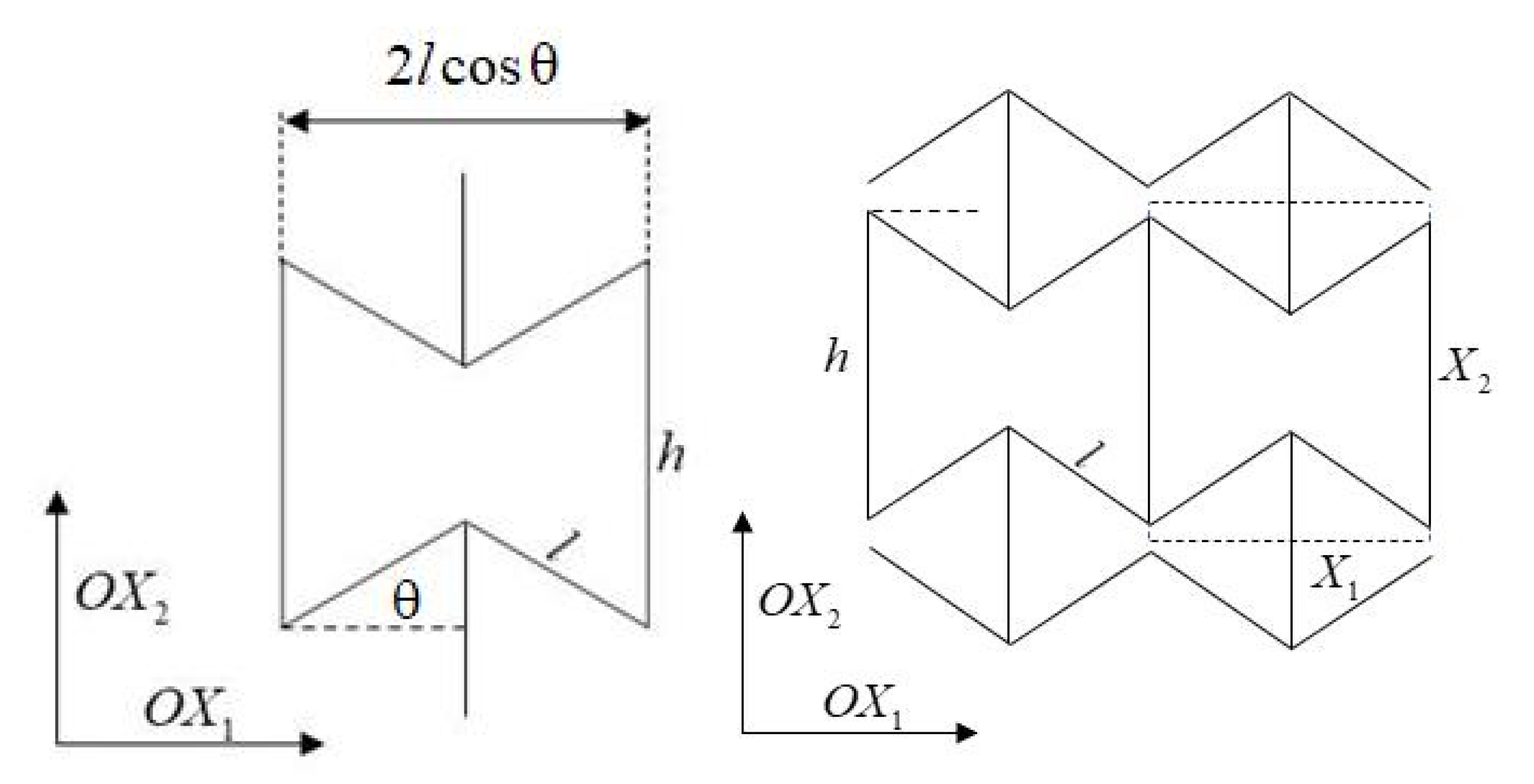
2.1. Theoretical Derivation of Poisson’s Ratio

Figure 1 shows the standard re-entrant hexagonal configuration of the honeycomb base:

$h$ and $l$ represent the length of the straight and hypotenuse sides of the structure, θ represents the re-entrant angle of the re-entrant structure and θ is negative. When the re-entrant hexagon configuration is loaded in the direction of OX₁ or OX₂ and is deformed in a linear elastic way, the dimension relation in the figure can be obtained from geometric relations:

$${\mathsf{\delta }}_1=2l\cos \mathsf{\theta }$$

(1)

$${\mathsf{\delta }}_2=h+2l\sin \mathsf{\theta }$$

(2)

It is assumed that the re-entrant element configuration is a rigid structure in the process of tiny deformation, that is, h and l are constant in the deformation process. The deformation of the re-entrant hexagonal element structure only depends on the change of the structural angle θ, which can be obtained from the Poisson’s ratio calculation formula. The Poisson’s ratio of the re-entrant structure is expressed as:

$$v=-\frac{\mathrm{d}{\mathsf{\delta }}_1}{\mathrm{d}{\mathsf{\delta }}_2}=-\frac{\mathrm{d}{\mathsf{\delta }}_1/\mathrm{d}\mathsf{\theta }}{\mathrm{d}{\mathsf{\delta }}_2/\mathrm{d}\mathsf{\theta }}\cdot \frac{{\mathsf{\delta }}_2}{{\mathsf{\delta }}_1}$$

(3)

The Poisson’s ratio expression of structure with respect to the re-entrant angle is expressed as:

$$v=\frac{(h/l+\sin \mathsf{\theta })\sin \mathsf{\theta }}{{\cos }^2\mathsf{\theta }}$$

(4)

According to Formula (4), we assume that the wall thickness of the re-entrant structure is constant and that Poisson’s ratio of the re-entrant hexagon varies with the re-entrant angle $\mathsf{\theta }$.

Figure 2 shows that Poisson’s ratio of the re-entrant hexagonal element structure decreases as the absolute value of the re-entrant angle increases. When the absolute value of the angle in the re-entrant hexagonal element is bigger than 30°, Poisson’s ratio changes minimally from 0 to −1. On the contrary, when the absolute value of the angle of the re-entrant hexagonal element is less than 30°, Poisson’s ratio increases rapidly as the absolute value of the angle decreases, and the range of Poisson’s ratio of the re-entrant hexagonal element is wider.

2.2. Honeycomb Base Modeling

A simple schematic diagram of a single re-entrant structure is given in Figure 3, where h and l are the length of the straight and hypotenuse sides of the re-entrant structure, respectively, and the numbers marked in the figure successively indicate that each truss element forming the re-entrant structure is an articulated connection.

In this paper, the Lagrange equation is used to model and analyze the re-entrant structure. The Lagrange equation is:

$$\frac{d}{dt}\left(\frac{\partial L}{\partial {\dot{q}}_i}\right)-\frac{\partial L}{\partial q_i}=Q_i,(i=1,2,\dots ,6)$$

(5)

where L is the Lagrange function, defined as $L=T-V$, T represents the kinetic energy of the structure and V represents the potential energy of the structure. Where $q_i$ represents the coordinates of the rod, ${\dot{q}}_i$ represents the speed of the nodes in the structure, that is, the derivative of $q_i$ with respect to time t, and i represents the numbers of the nodes in the re-entrant structure. In order to conveniently calculate the kinetic energy and potential energy of the structure, the constant mass matrix in the finite element was introduced. The schematic diagram of the space truss element is given in Figure 4.

The node displacement component $Q^e$ of the truss element in the global coordinate system can be expressed as:

$$Q^e=[Q_{3i-2}{Q}_{3i-1}{Q}_{3i}{Q}_{3j-2}{Q}_{3j-1}{Q}_{3j}]$$

(6)

where i represents the number of endpoints of a cell.

Assume that the linear displacement mode was:

$$U(x)={[u(x)v(x)w(x)]}^T=N{Q}^e$$

(7)

In Formula (7), N is a 3 × 6 function:

$$N=\left[\begin{array}{cccccc}\frac{l-x}{l}& 0& 0& \frac{x}{l}& 0& 0\\ 0& \frac{l-x}{l}& 0& 0& \frac{x}{l}& 0\\ 0& 0& \frac{l-x}{l}& 0& 0& \frac{x}{l}\end{array}\right]$$

(8)

If the density $\mathsf{\rho }$ and the cross-sectional area $A$ were constant, the uniform mass matrix of space truss elements in the global coordinate system can be obtained:

$$M^e(or{m}^e)={\displaystyle \underset{V^e}{\iiint }\mathsf{\rho }{N}^{T}N\mathrm{d}V}$$

(9)

Substitute Formula (8) into Formula (9) to obtain:

$$M^e={\displaystyle {\iiint }_{V^e}\mathsf{\rho }}{N}^{T}NdV=\frac{\mathsf{\rho }Al}{6}\left[\begin{array}{cccccc}2& 0& 0& 1& 0& 0\\ 0& 2& 0& 0& 1& 0\\ 0& 0& 2& 0& 0& 1\\ 1& 0& 0& 2& 0& 0\\ 0& 1& 0& 0& 2& 0\\ 0& 0& 1& 0& 0& 2\end{array}\right]$$

(10)

Thus, the uniform mass matrix of space truss elements was obtained. The kinetic energy equation is expressed as:

$$T=\frac{1}{2}\dot{X}{M}^e{\dot{X}}^T$$

(11)

In Formula (11), $\dot{X}$ represents the speed of the bar of the re-entrant structure, that is, the derivative of the displacement $X$ with respect to time t. ${\dot{X}}^T$ represents the Transposed matrix of the $\dot{X}$.

The overall kinetic energy of the re-entrant structure can be obtained by substituting the node coordinates of the re-entrant structure and the uniform mass matrix. Here, truss 12 in the re-entrant structure is used as an example to give the specific expression used to determine the kinetic energy of the truss. Other trusses can be obtained by the same method when used successively, according to Formulas (9) and (10). The kinetic energy of the truss 12 is expressed as follows:

$$T_{12}=\frac{\mathsf{\rho }Al}{6}\left({\dot{x}}_1^2+{\dot{x}}_1{\dot{x}}_2+{\dot{x}}_2^2+{\dot{y}}_1^2+{\dot{y}}_1{\dot{y}}_2+{\dot{y}}_2^2+{\dot{z}}_1^2+{\dot{z}}_1{\dot{z}}_2+{\dot{z}}_2^2\right)$$

(12)

where ${\dot{x}}_i,{\dot{y}}_i,{\dot{z}}_i,i=1,2$ represents the derivative with respect to time t of the coordinate position of a node in a spatial coordinate system, that is, the derivative of the coordinates $x_i,y_i,z_i,i=1,2$ with respect to time t. According to Formula (12), the kinetic energy of the other trusses can be obtained. The sum of the kinetic energy of all the trusses is the kinetic energy of the system.

The elastic potential energy of the space truss element is expressed as follows:

$$V_1=\frac{1}{2}{{\displaystyle {\int }_0^{l}E\left(\frac{{\partial }^{2}y}{{\partial }^{2}x}\right)}}^2\mathrm{d}x=\frac{1}{2}{X}^T{K}^{e}X$$

(13)

$$V_1={\displaystyle {\int }_0^{l}EAN{N}^T\mathrm{d}x}=\frac{1}{2}{X}^T{K}^{e}X$$

(14)

In Formula (13) and (14), $X$ is the coordinate matrix of the truss that contains the x, y and z coordinates. $K^e$ is the stiffness matrix of the truss element and is expressed as follows:

$$K^e={\displaystyle {\int }_0^{l}EAN{N}^T\mathrm{d}x}=\frac{EA}{l}\left[\begin{array}{cccccc}1& 0& 0& -1& 0& 0\\ 0& 1& 0& 0& -1& 0\\ 0& 0& 1& 0& 0& -1\\ -1& 0& 0& -1& 0& 0\\ 0& -1& 0& 0& -1& 0\\ 0& 0& -1& 0& 0& -1\end{array}\right]$$

(15)

where l represents the length of the truss in the structure. By substituting Formula (15) into Formulas (13) and (14), and using rod 12 as an example, the elastic potential energy formula can be obtained as follows:

$$V_{12}=\frac{EA}{2l}\left(x_1{}^2-2x_1{x}_2-x_2{}^2+y_1{}^2-2y_1{y}_2-y_2{}^2+z_1{}^2-2z_1{z}_2-z_2{}^2\right)$$

(16)

where $x_i,y_i,z_i,i=1,2$ represents the coordinate position of a node in a spatial coordinate system. According to Formula (16), the potential energy of the other truss can be obtained and the sum of the potential energy $V_1$ of all the trusses is the kinetic energy of the system.

The gravitational potential energy of the structure can be expressed as:

$$V_2={\displaystyle {\int }_0^l{M}^{e}g\mathrm{d}x}=\frac{1}{2}{X}^T{M}^{e}gX$$

(17)

where X represents the displacement component of the rod in the structure. Formula (10) is substituted into Formula (17) to obtain the gravitational potential energy of each rod:

$$V_{{12}^{\prime }}=\frac{\mathsf{\rho }Alg}{6}\left(x_1^2+x_1{x}_2+x_2^2+y_1^2+y_1{y}_2+y_2^2+z_1^2+z_1{z}_2+z_2^2\right)$$

(18)

where $x_i,y_i,z_i,i=1,2$ represents the coordinate position of a node in a spatial coordinate system. According to Formula (18), the gravitational potential energy of the other truss can be obtained and the sum of the gravitational potential energy $V_2$ of all the trusses is the kinetic energy of the system.

The Lagrange function L of the structure can be obtained from the kinetic energy and potential energy of the structure: $L=T-V$ and $V=V_1+V_2$.

The external force of the negative Poisson’s ratio re-entrant structure is:

$$Q_i=Q_1+Q_2+Q_3$$

(19)

where, $Q_1$ refers to the external incentives received by the structure:

$$Q_1=f\left(t\right)=F\sin \mathsf{\omega }t$$

(20)

For the connection mode of each node, $Q_2$ represents the damping force of the structure:

$$Q_2=\frac{\partial D}{\partial {\dot{q}}_i}=-{\displaystyle \sum _{j=1}^n{c}_{ij}{\dot{q}}_j}$$

(21)

where C_cj is the damping coefficient at the hinge point and ${\dot{q}}_j$ is the speed of the $q_j$, that is, the derivative of the coordinates $q_j$ with respect to time t. This paper only explores the dynamic influence of external excitation on the structure. In order to facilitate this calculation, a fixed friction force is given at each node to offset the gravity of the honeycomb base structure itself.

$$Q_2=-Q_3$$

(22)

where $Q_3$ is the force of gravity on the rod.

The constraint equation of the system was introduced and Formula (4) can be written in matrix form as follows. Formula (23) is the differential algebraic equation for the honeycomb base:

$$\left[\begin{array}{cc}M& {\mathsf{\Phi }}_q{}^T\\ {\mathsf{\Phi }}_q& 0\end{array}\right]\left[\begin{array}{c}\ddot{q}\\ \lambda \end{array}\right]=\left[\begin{array}{c}F(q,\dot{q},t)\\ -{\mathsf{\Phi }}_q(q,t)\ddot{q}-{({\mathsf{\Phi }}_q(q,t)\dot{q})}_q\dot{q}-2{\mathsf{\Phi }}_{qt}(q,t)\dot{q}-{\mathsf{\Phi }}_{tt}(q,t)\end{array}\right]$$

(23)

where $\dot{q}$ is the speed of the coordinate $q$, that is, the derivative of the coordinate $q$ with respect to time t, and $\ddot{q}$ is the acceleration of the coordinate $q$, that is, the second derivative of the coordinate $q$ with respect to time t. Where ${\mathsf{\Phi }}_q$ is the derivative of $\mathsf{\Phi }$ with respect to $q$, and ${\mathsf{\Phi }}_{qt}$ is the derivative of the $\mathsf{\Phi }$ with respect to $q$ and t, ${\mathsf{\Phi }}_{tt}$ is the second derivative of the $\mathsf{\Phi }$ with respect to time t. Taking a single re-entrant element as an example, as is shown in Figure 3, the coordinate of each node can be obtained:

$$q_1=\left[\begin{array}{ccc}{x}_1& y_1& z_1\end{array}\right]=\left[\begin{array}{ccc}0& 0& 0\end{array}\right]$$

(24)

$$q_2=\left[\begin{array}{ccc}{x}_2& y_2& z_2\end{array}\right]=\left[\begin{array}{ccc}0& l\cos \mathsf{\alpha }& l\sin \mathsf{\alpha }\end{array}\right]$$

(25)

$$q_3=\left[\begin{array}{ccc}{x}_3& y_3& z_3\end{array}\right]=\left[\begin{array}{ccc}0& 0& 2l\sin \mathsf{\alpha }\end{array}\right]$$

(26)

$$q_4=\left[\begin{array}{ccc}{x}_4& y_4& z_4\end{array}\right]=\left[\begin{array}{ccc}0& h& 2l\sin \mathsf{\alpha }\end{array}\right]$$

(27)

$$q_5=\left[\begin{array}{ccc}{x}_5& y_5& z_5\end{array}\right]=\left[\begin{array}{ccc}0& h-l\cos \mathsf{\alpha }& l\sin \mathsf{\alpha }\end{array}\right]$$

(28)

$$q_6=\left[\begin{array}{ccc}{x}_6& y_6& z_6\end{array}\right]=\left[\begin{array}{ccc}0& h& 0\end{array}\right]$$

(29)

Each node does not exist independently of the negative Poisson’s ratio re-entrant structure. There are certain constraints among the structure nodes. The constraint $\mathsf{\Phi }$ of Formula (23) is as follows. In Formula (23), ${\mathsf{\Phi }}_q$ represents the Jacobian matrix for the coordinate matrix q.

$${\mathsf{\Phi }}_1=\left(\begin{array}{c}{\left(x_1-x_2\right)}^2+{\left(y_1-y_2\right)}^2+{\left(z_1-z_2\right)}^2-l^2\\ {\left(x_3-x_2\right)}^2+{\left(y_3-y_2\right)}^2+{\left(z_3-z_2\right)}^2-l^2\\ {\left(x_4-x_3\right)}^2+{\left(y_4-y_3\right)}^2+{\left(z_4-z_3\right)}^2-h^2\\ {\left(x_5-x_4\right)}^2+{\left(y_5-y_4\right)}^2+{\left(z_5-z_4\right)}^2-l^2\\ {\left(x_6-x_5\right)}^2+{\left(y_6-y_5\right)}^2+{\left(z_6-z_5\right)}^2-l^2\\ {\left(x_1-x_6\right)}^2+{\left(y_1-y_6\right)}^2+{\left(z_1-z_6\right)}^2-h^2\end{array}\right)=0$$

(30)

where $x_i,y_i,z_i,i=1,2$ represents the coordinate position of a node in a spatial coordinate system. Formula (30) and the Lagrange function L was substituted into Formula (23) to obtain the mass matrix of the entire structure, that is, the mass matrix in Formula (23):

$$M=\left[\begin{array}{cccccccccccc}{M}_1& M_2& 0& 0& 0& M_3& M_5& M_6& 0& 0& 0& M_7\\ M_2& M_4& M_2& 0& 0& 0& M_{10}& M_4& M_7& M_9& M_9& 0\\ 0& M_2& M_1& M_2& 0& 0& 0& M_{10}& M_8& 0& 0& 0\\ 0& 0& M_2& M_1& M_2& 0& M_{10}& 0& M_7& M_8& M_7& 0\\ 0& 0& 0& M_2& M_4& M_2& 0& 0& 0& M_6& M_4& M_7\\ M_3& 0& 0& 0& M_2& M_1& M_7& 0& 0& 0& M_6& M_8\end{array}\right]$$

(31)

where M is composed of different small matrices. Each small matrix is expressed in Appendix A.

In the small matrices shown in Appendix A. E represents the elastic modulus of the re-entrant structure and $l$ represents the length of the truss. The small matrices that make up the M-matrix are all symmetric matrices.

For the entire honeycomb base, as shown in Figure 5.

The honeycomb base consists of six layers and three rows of negative Poisson’s ratio re-entrant structures. The whole base is symmetrical. The number of $q$ in the whole model, that is, the number of nodes, is:

$$2m\left[6+4\left(n-1\right)\right]$$

(32)

The number of constraint equations, that is, the number of equations of the constraint matrix $\mathsf{\Phi }$, is as follows:

$$2m\left[6+4\left(n-1\right)\right]+2\left[m\left(5n+1\right)+n(m-1)\right]$$

(33)

where m represents the number of columns and n represents the number of layers of the re-entrant structure of the honeycomb base. The dynamic equation of the whole honeycomb base can be obtained, and the constraint matrix and mass matrix of the whole honeycomb base can be obtained by combining Formulas (32) and (33). For the coordinates of the nodes when n > 1, the number of nodes increases by 4 for each additional layer. Take the second layer as an example; the number of nodes increased by 7, 8, 9 and 10. The coordinates of the node can be obtained as follows:

$$q_{1+6(n-1)}=\left[\begin{array}{ccc}{x}_{1+6(n-1)}& y_{1+6(n-1)}& z_{1+6(n-1)}\end{array}\right]=\left[\begin{array}{ccc}0& l\cos \mathsf{\alpha }& (n+1)l\sin \mathsf{\alpha }\end{array}\right]$$

(34)

$$q_{2+6(n-1)}=\left[\begin{array}{ccc}{x}_{2+6(n-1)}& y_{2+6(n-1)}& z_{2+6(n-1)}\end{array}\right]=\left[\begin{array}{ccc}0& 0& (n+2)l\sin \mathsf{\alpha }\end{array}\right]$$

(35)

$$q_{3+6(n-1)}=\left[\begin{array}{ccc}{x}_{3+6(n-1)}& y_{3+6(n-1)}& z_{3+6(n-1)}\end{array}\right]=\left[\begin{array}{ccc}0& h& (n+2)l\sin \mathsf{\alpha }\end{array}\right]$$

(36)

$$q_{4+6(n-1)}=\left[\begin{array}{ccc}{x}_{4+6(n-1)}& y_{4+6(n-1)}& z_{4+6(n-1)}\end{array}\right]=\left[\begin{array}{ccc}0& h-l\cos \mathsf{\alpha }& (n+1)l\sin \mathsf{\alpha }\end{array}\right]$$

(37)

where $\mathsf{\alpha }=\frac{\pi }{2}-\left|\mathsf{\theta }\right|$.

When m > 1, the number of nodes increases by 6 for each additional column, and the number of nodes starts from the last one in the first column, i.e., the first node in the second column should be $q_{(m-1)(4+6(n-1))+1}$. The coordinates of nodes in each column can be expressed as:

$$q_{(m-1)(4+6(n-1))+1}=\left[\begin{array}{ccc}0& 2(m-1)(h-l\cos \mathsf{\alpha })& 0\end{array}\right]$$

(38)

$$q_{(m-1)(4+6(n-1))+2}=\left[\begin{array}{ccc}0& 2(m-1)(h-l\cos \mathsf{\alpha })+l\cos \mathsf{\alpha }& l\sin \mathsf{\alpha }\end{array}\right]$$

(39)

$$q_{(m-1)(4+6(n-1))+3}=\left[\begin{array}{ccc}0& 2(m-1)(h-l\cos \mathsf{\alpha })& 2l\sin \mathsf{\alpha }\end{array}\right]$$

(40)

$$q_{(m-1)(4+6(n-1))+4}=\left[\begin{array}{ccc}0& 2(m-1)(h-l\cos \mathsf{\alpha })+h& 2l\sin \mathsf{\alpha }\end{array}\right]$$

(41)

$$q_{(m-1)(4+6(n-1))+5}=\left[\begin{array}{ccc}0& 3(m-1)(h-l\cos \mathsf{\alpha })& l\sin \mathsf{\alpha }\end{array}\right]$$

(42)

$$q_{(m-1)(4+6(n-1))+6}=\left[\begin{array}{ccc}0& 3(m-1)(h-l\cos \mathsf{\alpha })+l\cos \mathsf{\alpha }& 0\end{array}\right]$$

(43)

The coordinates of the n layer in the m column can be deduced by combining Formulas (38) to (43). As the stiffness and strength of the base are taken into consideration, steel was selected as the material constituting the honeycomb base. Its material coefficients are expressed as follows:

$$E=210\mathrm{G}\mathrm{p}\mathrm{a},v=0.3,\mathsf{\rho }=7800{\mathrm{kg}/\mathrm{m}}^3$$

(44)

3. Numerical Results Analysis

The vibration level difference was used to evaluate the vibration reduction performance of the honeycomb base, which is defined as the ratio of the acceleration response at corresponding points in the upper and lower planes, and is expressed as follows:

$$L_r=20\lg \frac{a_{up}}{a_{down}}$$

(45)

where $a_{up}$ and $a_{down}$ are the average accelerations at the upper and lower plane nodes, respectively. A simple harmonic external force with an amplitude of 100 N was applied to the mechanism, and the vibration level difference diagram under different parameters of the re-entrant structure of the mechanism was obtained. Due to the long duration of solution stability, the discrete variational method [28] was used to calculate Formula (21) of the honeycomb base. Here, the thickness of the cross-section of the truss was used to represent the area of the cross-section so as to more intuitively analyze the influence of the thickness of the truss on the vibration level difference (in this paper, h = 10 cm and l = 5 cm).

Figure 6 shows the vibration level difference diagram of the re-entrant element of the honeycomb base when the external excitation frequency was 10 Hz: (a) when the wall thickness of the re-entrant structure was $\mathsf{\tau }=0.1\mathrm{c}\mathrm{m}$, (b) when the wall thickness of the re-entrant structure was $\mathsf{\tau }=0.2\mathrm{c}\mathrm{m}$.

Figure 7 shows the vibration level difference diagram of the re-entrant element of the honeycomb base when the external excitation frequency was 60 Hz: (a) when the wall thickness of the re-entrant structure was $\mathsf{\tau }=0.1\mathrm{c}\mathrm{m}$ and (b) when the wall thickness of the re-entrant structure was $\mathsf{\tau }=0.2\mathrm{c}\mathrm{m}$.

Figure 8 shows the vibration level difference diagram of the re-entrant element of the honeycomb base when the external excitation frequency was 110 Hz: (a) when the wall thickness of the re-entrant structure was $\mathsf{\tau }=0.1\mathrm{c}\mathrm{m}$ and (b) when the wall thickness of the re-entrant structure was $\mathsf{\tau }=0.2\mathrm{c}\mathrm{m}$.

The vibration level differences are given in

Table 1. $v=-0.47$ vibration level differences at different frequencies of excitation.

${\mathit{L}}_{\mathit{r}}(\mathbf{d}\mathbf{b})$	${\mathit{L}}_{\mathit{r}}(\mathbf{d}\mathbf{b})\left[10\mathbf{Hz}\right]$	${\mathit{L}}_{\mathit{r}}(\mathbf{d}\mathbf{b})\left[60\mathbf{Hz}\right]$	${\mathit{L}}_{\mathit{r}}(\mathbf{d}\mathbf{b})\left[110\mathbf{Hz}\right]$
$\mathsf{\tau }=0.1\mathrm{c}\mathrm{m}$	0.1776	4.6000	0.0355
$\mathsf{\tau }=0.2\mathrm{c}\mathrm{m}$	0.1776	0.1196	5.5000

. These data were obtained when the honeycomb base was composed of a re-entrant structure with a Poisson’s ratio of $v=-0.47$.

Figure 9 shows the vibration level difference diagram of the re-entrant element of the honeycomb base when the external excitation frequency was 10 Hz: (a) when the wall thickness of the re-entrant structure was $\mathsf{\tau }=0.1\mathrm{c}\mathrm{m}$ and (b) when the wall thickness of the re-entrant structure was $\mathsf{\tau }=0.2\mathrm{c}\mathrm{m}$.

Figure 10 shows the vibration level difference diagram of the re-entrant element of the honeycomb base when the external excitation frequency was 60 Hz: (a) when the wall thickness of the re-entrant structure was $\mathsf{\tau }=0.1\mathrm{c}\mathrm{m}$ and (b) when the wall thickness of the re-entrant structure was $\mathsf{\tau }=0.2\mathrm{c}\mathrm{m}$.

Figure 11 shows the vibration level difference diagram of the re-entrant element of the honeycomb base when the external excitation frequency was 110 Hz: (a) when the wall thickness of the re-entrant structure was $\mathsf{\tau }=0.1\mathrm{c}\mathrm{m}$ and (b) when the wall thickness of the re-entrant structure was $\mathsf{\tau }=0.2\mathrm{c}\mathrm{m}$.

The vibration level differences are given in

Table 2. $v=-1.11$ vibration level differences at different frequencies of excitation.

${\mathit{L}}_{\mathit{r}}(\mathbf{d}\mathbf{b})$	${\mathit{L}}_{\mathit{r}}(\mathbf{d}\mathbf{b})\left[10\mathbf{Hz}\right]$	${\mathit{L}}_{\mathit{r}}(\mathbf{d}\mathbf{b})\left[60\mathbf{Hz}\right]$	${\mathit{L}}_{\mathit{r}}(\mathbf{d}\mathbf{b})\left[110\mathbf{Hz}\right]$
$\mathsf{\tau }=0.1\mathrm{c}\mathrm{m}$	0.3963	4.7000	0.0792
$\mathsf{\tau }=0.2\mathrm{cm}$	0.3962	0.3300	5.5000

. These data were obtained when the honeycomb base was composed of a re-entrant structure with a Poisson’s ratio of $v=-1.11$.

In Figure 12, Figure 13 and Figure 14, the honeycomb base is composed of re-entrant structures with different Poisson ratios; the Poisson’s ratio of the re-entrant structure forming the three layers above the base was $v=-1.11$ and the Poisson’s ratio of the concave structure of the lower three layers was $v=-0.47$.

Figure 12 shows the vibration level difference diagram of the re-entrant element of the honeycomb base when the external excitation frequency was 10 Hz: (a) when the wall thickness of the re-entrant structure was $\mathsf{\tau }=0.1\mathrm{c}\mathrm{m}$ and (b) when the wall thickness of the re-entrant structure was $\mathsf{\tau }=0.2\mathrm{c}\mathrm{m}$.

Figure 13 shows the vibration level difference diagram of the re-entrant element of the honeycomb base when the external excitation frequency was 60 Hz: (a) when the wall thickness of the re-entrant structure was $\mathsf{\tau }=0.1\mathrm{c}\mathrm{m}$ and (b) when the wall thickness of the re-entrant structure was $\mathsf{\tau }=0.2\mathrm{c}\mathrm{m}$.

Figure 14 shows the vibration level difference diagram of the re-entrant element of the honeycomb base when the external excitation frequency was 110 Hz: (a) when the wall thickness of the re-entrant structure was $\mathsf{\tau }=0.1\mathrm{c}\mathrm{m}$ and (b) when the wall thickness of the re-entrant structure was $\mathsf{\tau }=0.2\mathrm{c}\mathrm{m}$.

The average values of the vibration level differences of the honeycomb base under different frequencies of external excitation are given in

Table 3. Vibration level differences at different frequencies with different Poisson’s ratios.

${\mathit{L}}_{\mathit{r}}(\mathbf{d}\mathbf{b})$	${\mathit{L}}_{\mathit{r}}(\mathbf{d}\mathbf{b})\left[10\mathbf{Hz}\right]$	${\mathit{L}}_{\mathit{r}}(\mathbf{d}\mathbf{b})\left[60\mathbf{Hz}\right]$	${\mathit{L}}_{\mathit{r}}(\mathbf{d}\mathbf{b})\left[110\mathbf{Hz}\right]$
$\mathsf{\tau }=0.1\mathrm{c}\mathrm{m}$	0.1869	4.7500	0.0792
$\mathsf{\tau }=0.2\mathrm{c}\mathrm{m}$	0.1691	0.0792	3.3500

. These data were obtained when different Poisson’s ratios were used.

From Table 1, Table 2 and Table 3 and Figure 6, Figure 7, Figure 8, Figure 9, Figure 10, Figure 11, Figure 12, Figure 13 and Figure 14, we drew the following conclusions:

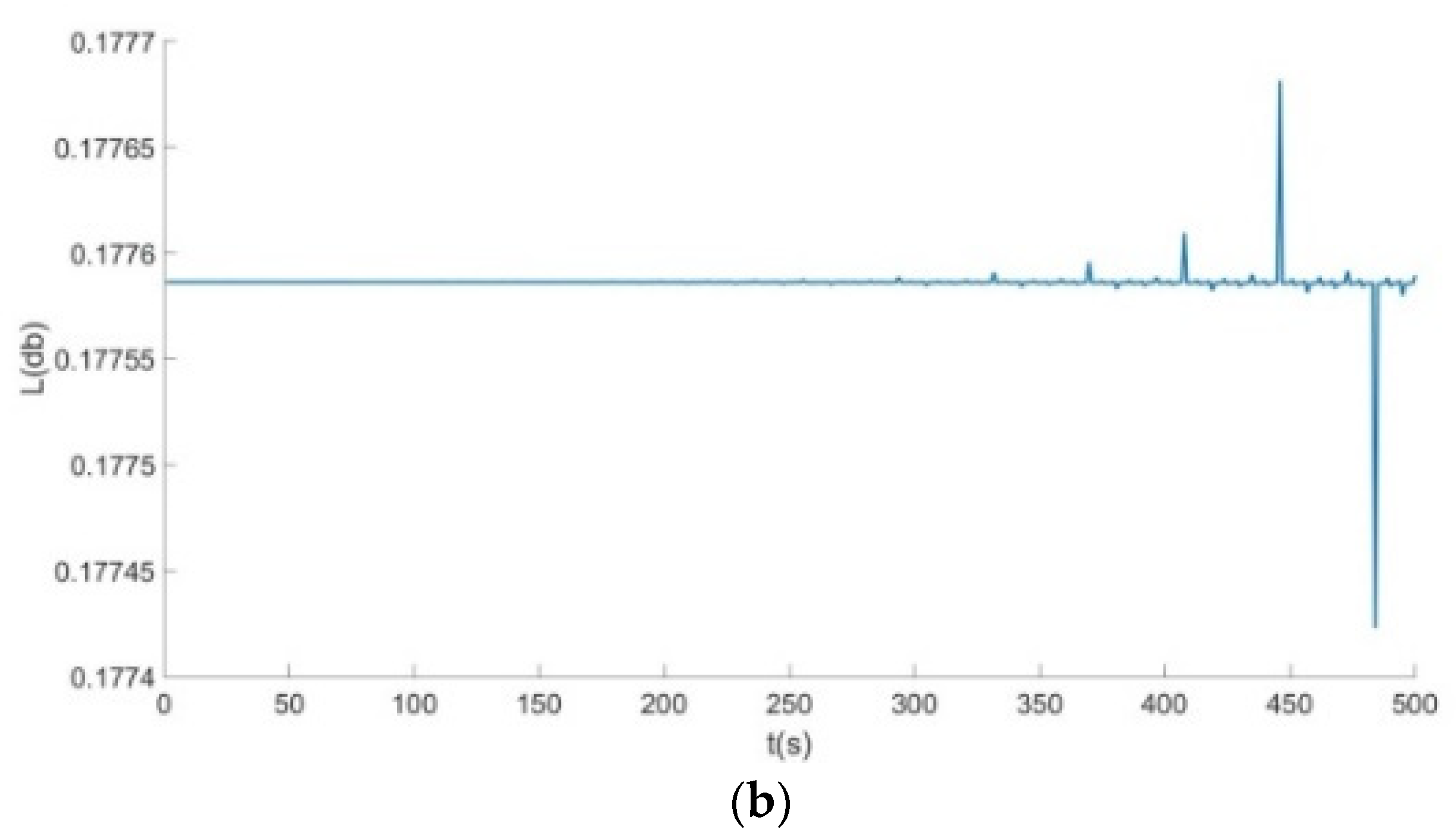
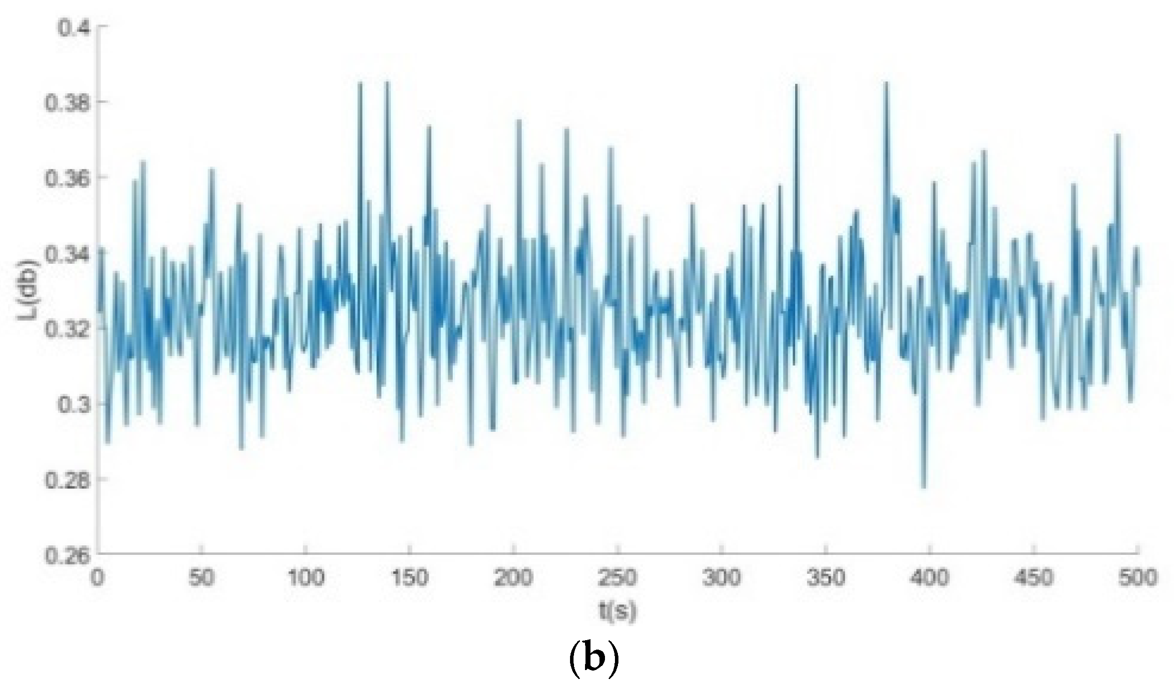
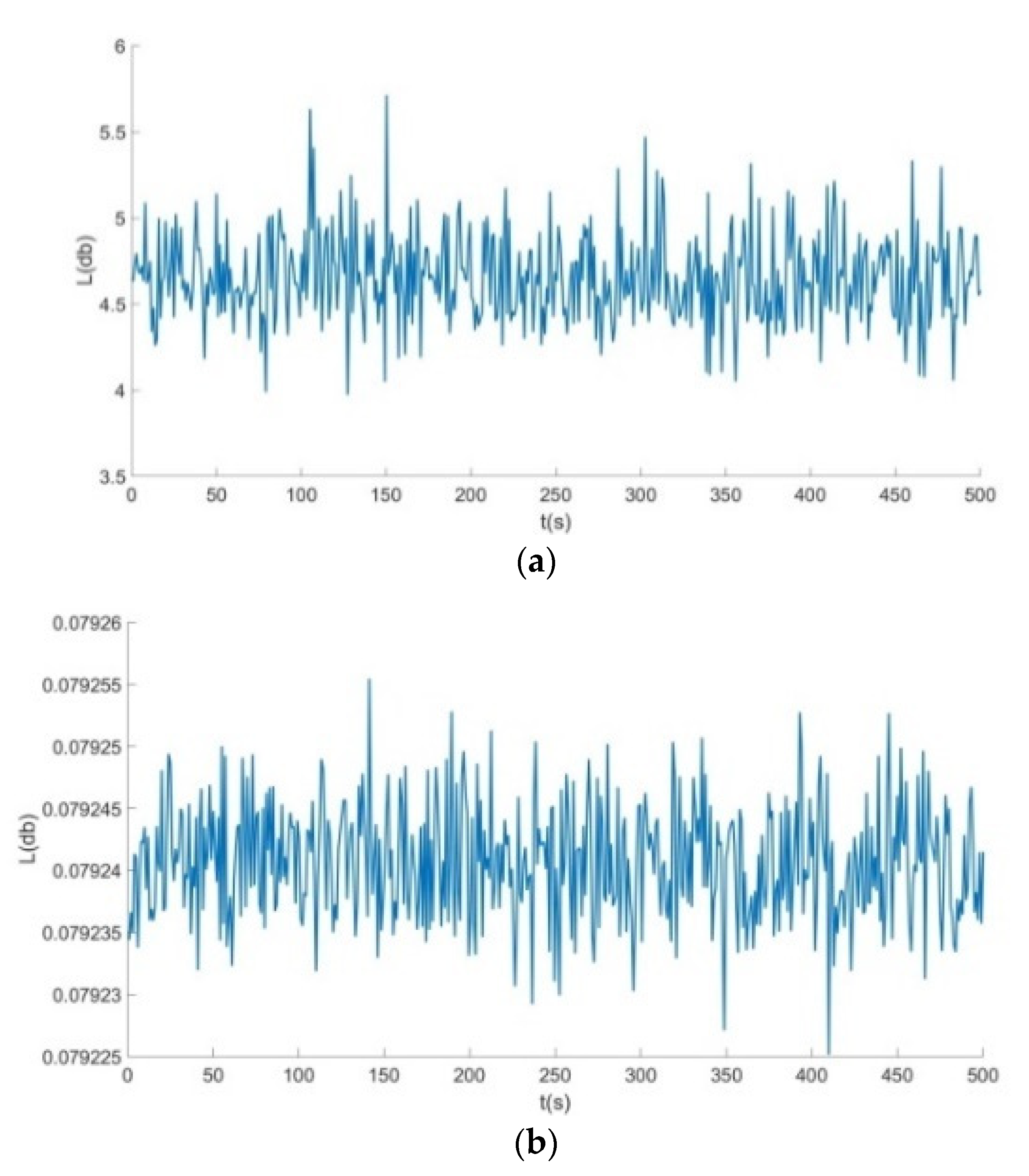
• From Figure 6, Figure 7 and Figure 8: when the Poisson’s ratio of the re-entrant structure was $v=-0.47$ and the wall thickness was $\mathsf{\tau }=0.1\mathrm{c}\mathrm{m}$, the honeycomb base had a better damping effect on the external excitation frequency of 60 Hz, but it had no obvious damping effects on the external excitation frequencies of 10 Hz and 120 Hz. When the wall thickness of the re-entrant structure was $\mathsf{\tau }=0.2\mathrm{c}\mathrm{m}$, the honeycomb base had an obvious damping effect on the external excitation frequency of 110 Hz, but it had no obvious damping effect on the low frequency of 10 Hz and the intermediate frequency of 60 Hz.
• From Figure 9, Figure 10 and Figure 11: when the Poisson’s ratio of the re-entrant structure was $v=-1.11$ and the wall thickness was $\mathsf{\tau }=0.1\mathrm{c}\mathrm{m}$, the honeycomb base had a better damping effect on the external excitation frequency of 60 Hz, but it had no obvious damping effects on the external excitation frequencies of 10 Hz and 120 Hz. When the wall thickness of the re-entrant structure was $\mathsf{\tau }=0.2\mathrm{c}\mathrm{m}$, the honeycomb base had an obvious damping effect on the external excitation frequency of 110 Hz, but it had no obvious damping effect on the low frequency of 10 Hz and the intermediate frequency of 60 Hz.
• From Figure 12, Figure 13 and Figure 14: when the re-entrant structure with mixed Poisson’s ratios was used to form the honeycomb base and when the wall thickness of the re-entrant structure was $\mathsf{\tau }=0.1\mathrm{c}\mathrm{m}$, the honeycomb base had a better damping effect on the external excitation frequency of 60 Hz, but it had no obvious damping effects on the external excitation frequencies of 10 Hz and 110 Hz. When the wall thickness of the re-entrant structure was $\mathsf{\tau }=0.2\mathrm{c}\mathrm{m}$, the honeycomb base had an obvious damping effect on the external excitation frequency of 120 Hz, but it had no obvious damping effect on the low frequency of 10 Hz and the middle frequency of 60 Hz.

The finite element COMSOL software was used to analyze the honeycomb base. The same size and material were selected for the re-entrant structure, and six layers were laid. In addition, an external excitation was applied to the top of the honeycomb base. The COMSOL software was used for meshing. A very fine grid was selected and the boundary conditions on the left and right sides of the base were continuous. By obtaining the frequency response curve of the honeycomb base, the isolation performance of the base in different frequency bands was analyzed. The ordinate represents the logarithm of the ratio of the end displacement of the honeycomb base to the initial displacement. Due to the isolation of the honeycomb base, when the ordinate value was less than 0, the honeycomb base isolated of the external excitation at this frequency well.

Figure 15 and Figure 16 show the frequency response curves of the honeycomb base when the wall thickness of the re-entrant structure was $\mathsf{\tau }=0.1\mathrm{c}\mathrm{m}$ and $\mathsf{\tau }=0.2\mathrm{c}\mathrm{m}$, respectively. The re-entrant angle of the structure was $\mathsf{\theta }=-15^{\circ }$ and the corresponding Poisson’s ratio was $v=-0.47$.

Figure 17 and Figure 18 show the frequency response curves of the honeycomb base when the wall thickness of the re-entrant structure was $\mathsf{\tau }=0.1\mathrm{c}\mathrm{m}$ and $\mathsf{\tau }=0.2\mathrm{c}\mathrm{m}$, respectively. The re-entrant angle of the re-entrant structure was $\mathsf{\theta }=-30^{\circ }$ and the corresponding Poisson’s ratio was $v=-1.11$.

Figure 19 and Figure 20 show the frequency response curves of the honeycomb base when the wall thickness of the re-entrant structure was $\mathsf{\tau }=0.1\mathrm{c}\mathrm{m}$ and $\mathsf{\tau }=0.2\mathrm{c}\mathrm{m}$, respectively. The honeycomb base was composed of two re-entrant structures with different Poisson’s ratios. The upper three layers were composed of a Poisson’s ratio of $v=-0.47$ and the lower three layers were composed of a Poisson’s ratio of $v=-1.11$.

From

Table 4. Vibration isolation frequencies of honeycomb bases under different parameters.

Vibration Isolation Frequency	$\mathit{v}=-0.47$	$\mathit{v}=-1.11$	$\mathit{v}=-0.47$$\mathit{v}=-1.11$
$\mathsf{\tau }=0.1\mathrm{c}\mathrm{m}$	60 Hz, 90 Hz–170 Hz	40 Hz–60 Hz	45 Hz–70 Hz
$\mathsf{\tau }=0.2\mathrm{c}\mathrm{m}$	125 Hz	75 Hz, 125 Hz	70 Hz–90 Hz, 120 Hz–150 Hz

and Figure 15, Figure 16, Figure 17, Figure 18, Figure 19 and Figure 20, we drew the following conclusions:

• By comparing the frequency response curves of the honeycomb base with different wall thicknesses of the re-entrant structure, we concluded that when the wall thickness was $\mathsf{\tau }=0.2\mathrm{c}\mathrm{m}$, the isolation frequency of the honeycomb base to external excitation was mainly concentrated on the relative high frequency. For example, when the Poisson’s ratio was $v=-0.47$, and the wall thickness was $\mathsf{\tau }=0.2\mathrm{c}\mathrm{m}$, the isolation frequency of the honeycomb base to external excitation was near a high frequency of 125 Hz. When Poisson’s ratio was $v=-1.11$, the vibration isolation frequency of the honeycomb base to external excitation was 125 Hz–150 Hz. When the honeycomb was laid with two different Poisson’s ratios, the vibration isolation frequency of the honeycomb base to external excitation was 70 Hz–90 Hz, 120 Hz–150 Hz and 180 Hz. In contrast, when the wall thickness of the re-entrant structure was $\mathsf{\tau }=0.1\mathrm{c}\mathrm{m}$, the vibration isolation frequency of the honeycomb base was mainly concentrated between 45 Hz–70 Hz.
• By analyzing the frequency response curves of the re-entrant hexagonal honeycomb structure with different Poisson’s ratios, we concluded that when Poisson’s ratio was $v=-1.11$, the vibration isolation performance of honeycomb base was better than that of the honeycomb base when Poisson’s ratio was $v=-0.47$.
• The method of laying the re-entrant structure with different Poisson’s ratios was adopted. By analyzing the corresponding frequency response curve, we concluded that the vibration isolation of the honeycomb base composed of re-entrant structures with different Poisson’s ratios to external excitation had a wider frequency band.
• By analyzing the results obtained using the Lagrange equation, we obtained the vibration isolation performance data and analyzed the honeycomb base by modeling the Lagrange equation, which was basically consistent with the results of the finite element analysis. Furthermore, this demonstrates the correctness and effectiveness of modeling and analyzing vibration isolation performance using the Lagrange method.

4. Conclusions

In this paper, the vibration isolation performance of honeycomb base with a negative Poisson’s ratio re-entrant structure was studied and analyzed. Lagrange equation modeling was used for the analysis. The finite element simulation COMSOL software was used for the experimental analysis. Through comparative analysis of the results, we concluded the following:

• By comparing the vibration level difference results of the honeycomb base composed of re-entrant structures with different Poisson’s ratios, we concluded that when the wall thickness of the re-entrant structure was $\mathsf{\tau }=0.1\mathrm{c}\mathrm{m}$, the honeycomb base had a better damping effect on the external excitation frequency of 60 Hz, but it had no obvious damping effects on the external excitation frequencies of 10 Hz and 120 Hz. When the wall thickness of the re-entrant structure was $\mathsf{\tau }=0.2\mathrm{c}\mathrm{m}$, the honeycomb base had an obvious damping effect on the external excitation at the high frequency of 110 Hz, but it had no obvious damping effect on the external excitation at the low frequency of 10 Hz and the intermediate frequency of 60 Hz.
• By comparing the frequency response curves of the honeycomb base with different wall thicknesses of the re-entrant structure, we concluded that when the wall thickness was $\mathsf{\tau }=0.2\mathrm{c}\mathrm{m}$, the isolation frequency of the honeycomb base to external excitation was mainly concentrated on the relative high frequency. In contrast, when the wall thickness of the re-entrant structure was $\mathsf{\tau }=0.1\mathrm{c}\mathrm{m}$, the vibration isolation frequency of the honeycomb base was more concentrated between 45 Hz–70 Hz. The method of laying the re-entrant structure with different Poisson’s ratios was adopted. By analyzing the corresponding frequency response curve, we concluded that the vibration isolation of the honeycomb base composed of re-entrant structures with different Poisson’s ratios to external excitation had a wider frequency band.

Numerical modeling is a more intuitive means of analyzing the vibration isolation performance of the honeycomb base and the re-entrant structure, and was used to analyze the effects of structural parameters on vibration isolation performance. The finite element consistent mass matrix was used to simplify the modeling calculations and to improve computational efficiency. COMSOL software was used for further verification of the analysis of the vibration isolation performance of the honeycomb base. The numerical modeling results were basically consistent with the results of the COMSOL software analysis, which also verifies the correctness of the numerical modeling method.

In terms of the practical applications of these findings for engineering, bases with better vibration isolation performance can be designed according to the contents of this paper, including the use of different structural parameters and Poisson ratios. Subsequently, 3D printers can be used to print the studied models for actual experimental analysis.

References

1. Hu, F.W.; Cheng, J.J. Reviews on metamaterials manufacturing via 3D printing. Ind. Technol. Innov. 2017, 4, 15–19. [Google Scholar]
2. Liu, W.W. Mechanics of Materials I; Higher Education Press: Beijing, China, 2004. [Google Scholar]
3. Shi, W.; Yang, W.; Li, Z.M. Advances in negative Poisson’s ratio materials. Polym. Bull. 2003, 6, 48–57. [Google Scholar]
4. Jiang, J.S.; Kim, Y.; Park, H.S. Auxetic nanomaterials, precent progress and future development. Appl. Phys. Rev. 2016, 3, 41101. [Google Scholar] [CrossRef] [Green Version]
5. Critchley, R.; Corni, I.; Wharton, J.A.F.; Walsh, C.; Wood, R.J.K.; Stokes, K.R. A review of the manufacture, mechanical properties and potential applications of auxetic foams. Phys. Status Solidi 2013, 250, 1963–1982. [Google Scholar] [CrossRef]
6. Evans, K.E.; Alderson, K.L. Auxetic materials, the positive side of being negative. Eng. Sci. Educ. J. 2000, 9, 148. [Google Scholar] [CrossRef]
7. Mir, M.; Ali, M.N.; Sami, J.; Ansari, U. Review of Mechanics and Applications of Auxetic Structures. Adv. Mater. Sci. Eng. 2014, 2014, 753496. [Google Scholar] [CrossRef] [Green Version]
8. Hassan, M.R.; Scarpa, F.; Mohamed, N.A. In-plane Tensile Behavior of Shape Memory Alloy Honeycombs with Positive and Negative Poisson’s Ratio. J. Intell. Mater. Syst. Struct. 2009, 20, 897–905. [Google Scholar]
9. Gibson, L.J.; Ashby, M.F.; Schajer, G.S. The Mechanics of two-dimensional cellular materials. Proc. R. Soc. A 1982, 382, 25–42. [Google Scholar]
10. Fozdar, D.Y.; Soman, P.; Lee, J.W. Three-dimensional polymer constructs exhibiting a tunable negative Poisson’s ratio. Adv. Funct. Mater. 2011, 21, 2712–2720. [Google Scholar] [CrossRef]
11. Gibson, L.J.; Ashby, M.F. Cellular Solids, Structure and Properties; Cambridge University Press: London, UK, 1997. [Google Scholar]
12. Scarpa, F.; Panayiotou, P.; Tomlinson, G. Numerical and experimental uniaxial loading on in-plane auxetic honeycombs. J. Strain Anal. Eng. Des. 2000, 35, 383–388. [Google Scholar] [CrossRef]
13. Alderson, K.L.; Alderson, A.; Smart, G. Auxetic polypropylene fibres, Part 1 Manufacture and character isation. Plast. Rubber Compos. 2013, 31, 344–349. [Google Scholar] [CrossRef]
14. Grima, J.N.; Gatt, R.; Alderson, A.; Evans, K.E. On the potential of connected stars as auxetic systems. Mol. Simul. 2005, 31, 925–935. [Google Scholar] [CrossRef] [Green Version]
15. Lim, T.C. Auxetic Materials and Structures; Springer: Singapore, 2015. [Google Scholar]
16. Wang, X.L.; Stronge, W.J. Micropolar theory for two-dimensional stresses in elastic honeycomb. Proc. R. Soc. A 1999, 455, 2091–2116. [Google Scholar] [CrossRef]
17. Sanami, M.; Ravirala, N.; Alderson, K.; Alderson, A. Auxetic materials for sports applications. Procedia Eng. 2014, 72, 453–458. [Google Scholar] [CrossRef] [Green Version]
18. Banerjee, S.; Bhaskar, A. Free vibration of cellular structures using continuum modes. J. Sound Vib. 2005, 287, 77–100. [Google Scholar] [CrossRef] [Green Version]
19. Ruzzene, M.; Scarpa, F.L. Control of wave propagation in sandwich beams with auxetic core. J. Intell. Mater. Syst. Struct. 2003, 14, 443–453. [Google Scholar] [CrossRef]
20. Idczak, E.; Strek, T. Computational modelling of vibrations transmission loss of auxetic lattice structure. Vib. Phys. Syst. 2016, 27, 123–128. [Google Scholar]
21. Ma, Y.; Scarpa, F.; Zhang, D.; Zhu, B.; Jie, H. A nonlinear auxetic structural vibration damper with metal rubber particles. Smart Mater. Struct. 2013, 22, 084012. [Google Scholar]
22. Grujicic, M.; Galgalikar, R.; Snipes, J.S. Multi-physics modeling of the fabrication and dynamic performance of all-metal auxetic-hexagonal sandwich-structures. Mater. Des. 2013, 51, 113–130. [Google Scholar] [CrossRef]
23. Qiao, J.; Chen, C.Q. Analyses on the In-Plane Impact Resistance of Auxetic Double Arrowhead Honeycombs. J. Appl. Mech. 2015, 82, 51007. [Google Scholar] [CrossRef]
24. Ingrole, A.; Hao, A.; Liang, R. Design and modeling of auxetic and hybrid honeycomb structures for in-plane property enhancement. Mater. Des. 2016, 117, 72–83. [Google Scholar] [CrossRef]
25. Schultz, J.; Griese, D.; Shankar, P.; Summers, J.D.; Thompson, L. Optimization of honeycomb cellular meso-structures for high speed impact energy absorption. In Proceedings of the ASME 2011 International Design Engineering Technical Conferences and Computers and Information in Engineering Conference, Washington, DC, USA, 28–31 August 2011. [Google Scholar]
26. Yu, Y.; Shen, H.S. A Comparison of Nonlinear Bending and Vibration of Hybrid Metal/CNTRC Laminated Beams with Positive and Negative Poisson’s Ratios. Int. J. Struct. Stab. Dyn. 2020, 20, 2043007. [Google Scholar] [CrossRef]
27. Lv, W.; Li, D.; Dong, L. Study on blast resistance of a composite sandwich panel with isotropic foam core with negative Poisson’s ratio. Int. J. Mech. Sci. 2021, 191, 106105. [Google Scholar] [CrossRef]
28. Pan, K.; Ding, J.Y.; Dong, H.W.; Zhang, B.B. Discrete variational method of multi-body system dynamics cased on center of gravity interpolation. J. Qingdao Univ. (Nat. Sci. Ed.) 2017, 30, 77–82. [Google Scholar]
Figure 1. Sketch of re-entrant structure.
Symmetry 14 01356 g001
Figure 2. Diagram of Poisson’s ratio of the re-entrant element changing with re-entrant angle (h/l = 2).
Symmetry 14 01356 g002
Figure 3. Schematic diagram of honeycomb base with re-entrant structure.
Symmetry 14 01356 g003
Figure 4. Space truss element.
Symmetry 14 01356 g004
Figure 5. Schematic diagram of the honeycomb base.
Symmetry 14 01356 g005
Figure 6. Vibration level difference diagram v = 0.47 , excitation frequency 10 Hz. (a) τ = 0.1   c m , (b) τ = 0.2   c m .
Symmetry 14 01356 g006aSymmetry 14 01356 g006b
Figure 7. Vibration level difference diagram v = 0.47 , excitation frequency 60 Hz. (a) τ = 0.1   c m , (b) τ = 0.2   c m .
Symmetry 14 01356 g007
Figure 8. Vibration level difference diagram v = 0.47 , excitation frequency 110 Hz. (a) τ = 0.1   c m , (b) τ = 0.2   c m .
Symmetry 14 01356 g008
Figure 9. Vibration level difference diagram v = 1.11 , excitation frequency 10 Hz. (a) τ = 0.1   c m , (b) τ = 0.2   c m .
Symmetry 14 01356 g009
Figure 10. Vibration level difference diagram v = 1.11 , excitation frequency 60 Hz. (a) τ = 0.1   c m , (b) τ = 0.2   c m .
Symmetry 14 01356 g010aSymmetry 14 01356 g010b
Figure 11. Vibration level difference diagram v = 1.11 , excitation frequency 110 Hz. (a) τ = 0.1   c m , (b) τ = 0.2   c m .
Symmetry 14 01356 g011
Figure 12. Vibration level difference diagram, excitation frequency 10 Hz. (a) τ = 0.1   c m , (b) τ = 0.2   c m .
Symmetry 14 01356 g012
Figure 13. Vibration level difference diagram, excitation frequency 60 Hz. (a) τ = 0.1   c m , (b) τ = 0.2   c m .
Symmetry 14 01356 g013
Figure 14. Vibration level difference diagram, excitation frequency 120 Hz. (a) τ = 0.1   c m , (b) τ = 0.2   c m .
Symmetry 14 01356 g014aSymmetry 14 01356 g014b
Figure 15. Frequency response curve of the base when the cell wall thickness was τ = 0.1   c m .
Symmetry 14 01356 g015
Figure 16. Frequency response curve of the base when the cell wall thickness was τ = 0.2   c m .
Symmetry 14 01356 g016
Figure 17. Frequency response curve of the base when the cell wall thickness was τ = 0.1   c m .
Symmetry 14 01356 g017
Figure 18. Frequency response curve of the base when the cell wall thickness was τ = 0.2   c m .
Symmetry 14 01356 g018
Figure 19. Frequency response curve of the base when the cell wall thickness was τ = 0.1   c m .
Symmetry 14 01356 g019
Figure 20. Frequency response curve of the base when the cell wall thickness was τ = 0.2   c m .
Symmetry 14 01356 g020