A Dynamic GLR-Based Fault Detection Method for Non-Gaussain Dynamic Processes

Abstract

Non-Gaussian dynamic processes are ubiquitous due to the presence of non-Gaussian distributed variables. Therefore, fault detection of non-Gaussian dynamic processes plays a vital role to maintain the safe operation of systems and symmetry of data distribution. In this paper, a dynamic generalized likelihood ratio (DGLR)-based fault detection method is proposed for non-Gaussian dynamic processes. Different from the conventional principal component analysis (PCA)-based, dynamic PCA-based, and PCA-based GLR fault detection methods, the novelty of the proposed method is that the GLR is extended to non-Gaussian dynamic processes, and the randomized algorithm is integrated for threshold setting to attenuate the influence of non-Gaussian. The application scope of these methods is also discussed. The proposed method is compared with four existing fault detection methods on a numerical simulation and the continuous stirred-tank reactor (CSTR) process. The achieved results show that the proposed method is able to significantly improve the detection performance in terms of fault detection rate and prompt response to faults.

1. Introduction

Fault detection is becoming increasingly important to maintain high quality products, operation safety of processes, and symmetry of data distribution. In recent years, considerable attention has been paid to research on solving fault detection problems. Model-based and data-driven methods are two common types [1,2,3,4,5,6]. In the model-based approaches, accurate physical or mathematical models are needed. On the other hand, in data-driven methods, only the availability of historical process data is required. Data-driven fault detection techniques have been widely used due to the simple application form and fewer requirements on development. The commonly used data-driven methods include generalized likelihood ratio (GLR)-based [7,8], multivariate analysis (MVA)-based, such as principal component analysis (PCA) [9,10,11,12], partial least square (PLS) [13,14,15], canonical correlation analysis (CCA) [16,17,18].

PCA is one of the most MVA techniques used for FD, which considers a single dataset. The successful application of such a method can be found in a wide range of applications, for example, dynamical, time varying, non-Gaussian and nonlinear processes [19]. Several variants of the standard PCA have been developed. These variants include dynamic PCA which is used to find dynamical linear relationships between the process variables [20], moving window PCA which handles time varying features [21], kernel density based-PCA which is used in non-Gaussian fault detection [22]. For GLR-based fault detection methods, some variants have also been developed in the fields of time varying [23], non-Gaussian [24], etc. However, the dynamic characteristic in process is rarely considered in the existing methods, and the better detection performance could be achieved by considering the auto-correlation characteristic in dynamic processes.

Furthermore, the successful application of the GLR-based method requires that the process data follows a Gaussian distribution. In practice, processes with non-Gaussian features put forward more challenges for fault detection. To this end, some variants of the existing fault detection methods have been developed. Commonly, there are two types of methods to deal with the fault detection problem for non-Gaussian processes. The first ones are either to use some methods, which are free of distribution, such as independent component analysis (ICA) [19] and support vector machine-based methods [25,26], or to extract high-order statistics and then use the standard method based on the obtained statistics [27]. For example, in [26], the ICA method is firstly used to get the independent components and then the support vector data description method is applied to generate a suitable threshold. The authors in [27] used various statistics to quantify process characteristics, such as non-Gaussian, furthermore monitoring these statistics instead of process variables themselves to perform fault detection. The second type of methods are first to estimate a probability distribution of the monitored variables or statistics, and then determine an appropriate threshold based on the resulting distribution. These methods can be referred to as distribution estimation-based methods [28]. A great number of methods have been developed for the estimation of distribution, including Gaussian Mixture Models (GMM) [29,30], kernel-based approaches [31,32] and sequential quantile estimation [33]. Motivated by the success of the second ones, in this paper, we use the same strategy. Although these existing methods are successful in this application domain, their performance in fault detection is commonly constrained by the determination of kernel structure and method-specified parameters, for example, the bandwidth parameter for a Gaussian kernel [31]. Therefore, due to the ability to iterative updating threshold, a randomized algorithm-based threshold learning method is used to enhance the dynamic GLR (DGLR)-based method to deal with the fault detection task in non-Gaussian dynamic processes.

Motivated by the above analysis, a DGLR-based fault detection method combined with the threshold learning method is proposed for non-Gaussian dynamic processes. The contribution of this work is four-fold: (1) to develop a DGLR-based detection statistic for non-Gaussian dynamic processes; (2) to improve DGLR-based fault detection performance by iteratively learning the suitable threshold by a randomized algorithm; (3) to compare the DGLR-based fault detection methods with the GLR-based, PCA-based, DPCA-based, and PCA-based GLR ones [34]. Based on our best knowledge, there are few works to compare these methods with the purpose to clarify the application scope of these method and to guide the practitioners to select a suitable fault detection method; (4) to assess the DGLR-based fault detection performance by comparing it with the GLR-based, PCA-based, DPCA-based, and PCA-based GLR methods using a numerical simulation and the continuous stirred-tank reactor (CSTR) process.

Notation 1.

The notation used in this paper is standard. ${\mathcal{R}}^n$ denotes the n-dimensional Euclidean space consisting of $n\times 1$ vectors with real components, ${\mathcal{R}}^{n\times m}$ is the set of all $n\times m$ real matrices, and $\mathit{diag}(\dots ,\dots ,\dots )$ is a square diagonal matrix. $\mathit{A}(:,i)$ represents the i-th column of $\mathit{A}$. ${\mathit{I}}_n$ is an $n\times n$ identity matrix. $\mathit{x}\sim \mathcal{N}\left({\mathbf{\mu }}_x,{\mathbf{\Sigma }}_x\right)$ denotes that x is a normally distributed random vector with mean ${\mathit{\mu }}_x$ and covariance ${\mathrm{\Sigma }}_x$. $E(·)$ denotes the expectation operator. ${\chi }^2\left(m\right)$ stands for the chi-square distribution with m degrees of freedom. Let $\mathit{pr}({\chi }^2>{\chi }_{\alpha }^2\left(m\right))=\alpha$ be the probability that ${\chi }^2>{\chi }_{\alpha }^2\left(m\right)$ equals α (significance level).

2. Background and Problem Formulation

2.1. The Basics of GLR-Based Fault Detection Technique

Consider the following fault detection problem using a GLR-based technique. Given a general model

$$\mathbf{y}={\mathbf{y}}^{*}+\mathbf{f}\in {\mathcal{R}}^m$$

(1)

where ${\mathbf{y}}^{*}\sim \mathcal{N}(0,\mathrm{\Sigma })$ represents the statistical features of the process and m is the dimension of the variable. Since $\mathbf{f}=0$ denotes the fault-free case, our task consists of detecting a fault $\mathbf{f}\ne 0$ with N number of available measurements of ${\mathbf{y}}_1,\dots ,{\mathbf{y}}_N$.

The fault detection task can be solved by testing the following hypotheses based on the available data $\mathbf{y}$ [7]

$$\begin{array}{cc}\hfill H_0,\mathrm{null}\mathrm{hypothesis}\text{:}\mathbf{f}& =0,\mathrm{fault}-\mathrm{free},\hfill \\ \hfill H_1,\mathrm{alternative}\mathrm{hypothesis}\text{:}\mathbf{f}& \ne 0,\mathrm{faulty}.\hfill \end{array}$$

The probability density functions (pdf) of ${\mathbf{y}}^{*}$ and $\mathbf{y}$ are respectively given as

$$\begin{array}{cc}\hfill P_0\left(\mathbf{y}\right)& =\frac{1}{\sqrt{{\left(2\pi \right)}^m}det\mathrm{\Sigma }}{exp}^{-0.5{\mathbf{y}}^T{\mathrm{\Sigma }}^{-1}\mathbf{y}},\hfill \end{array}$$

(2)

$$\begin{array}{cc}\hfill P_1\left(\mathbf{y}\right)& =\frac{1}{\sqrt{{\left(2\pi \right)}^m}det\mathrm{\Sigma }}{exp}^{-0.5({\mathbf{y}}^T-\mathrm{E}\left(\mathbf{y}\right)){\mathrm{\Sigma }}^{-1}(\mathbf{y}-\mathrm{E}\left(\mathbf{y}\right))},\hfill \end{array}$$

(3)

The log likelihood ratio is defined as

$$s\left(\mathbf{y}\right)=2ln\frac{P_1\left(\mathbf{y}\right)}{P_0\left(\mathbf{y}\right)}={\mathbf{y}}^T{\mathrm{\Sigma }}^{-1}\mathbf{y}-{(\mathbf{y}-\mathrm{E}\left(\mathbf{y}\right))}^T{\mathrm{\Sigma }}^{-1}(\mathbf{y}-\mathrm{E}\left(\mathbf{y}\right))$$

(4)

To increase the confidence of the decision-making procedure, generally more samples are required. Using N samples of data $\mathbf{y}$, Equation (4) is extended as

$$\begin{array}{cc}\hfill S_1^N& =\sum _{k=1}^{N}2ln\frac{P_1\left({\mathbf{y}}_k\right)}{P_0\left({\mathbf{y}}_k\right)}\hfill \\ \hfill & =\sum _{k=1}^N{\mathbf{y}}_k^T{\mathrm{\Sigma }}^{-1}\mathbf{y}-\sum _{k=1}^N{({\mathbf{y}}_k-\mathrm{E}\left(\mathbf{y}\right))}^T{\mathrm{\Sigma }}^{-1}({\mathbf{y}}_k-\mathrm{E}\left(\mathbf{y}\right))\hfill \\ \hfill & =2N{\overline{\mathbf{y}}}^T{\mathrm{\Sigma }}^{-1}\mathrm{E}\left(\mathbf{y}\right)-N\mathrm{E}{\left(\mathbf{y}\right)}^T{\mathrm{\Sigma }}^{-1}\mathrm{E}\left(\mathbf{y}\right),\overline{\mathbf{y}}=\frac{1}{N}\sum _{k=1}^N{\mathbf{y}}_k\hfill \\ \hfill & =N({\overline{\mathbf{y}}}^T{\mathrm{\Sigma }}^{-1}\overline{\mathbf{y}}-{(\overline{\mathbf{y}}-\mathrm{E}\left(\mathbf{y}\right))}^T{\mathrm{\Sigma }}^{-1}(\overline{\mathbf{y}}-\mathrm{E}\left(\mathbf{y}\right)))\hfill \end{array}$$

(5)

Evidently, the maximum of $S_1^N$ is

$$N{\overline{\mathbf{y}}}^T{\mathrm{\Sigma }}^{-1}\overline{\mathbf{y}}$$

(6)

when $\overline{\mathbf{y}}=\mathrm{E}\left(\mathbf{y}\right)$ is achieved. Since $\mathrm{E}\left(\mathbf{y}\right)$ is generally unknown, it can be replaced by its maximum likelihood estimate

$$\mathrm{E}\left(\mathbf{y}\right)=\frac{1}{N}\sum _{k=1}^N{\mathbf{y}}_k$$

(7)

In practice $\mathrm{\Sigma }$ is also unknown, which needs to be identified from the data. It is straightforward that

$$\underset{N\to \infty }{lim}\widehat{\mathrm{\Sigma }}=\underset{N\to \infty }{lim}\frac{1}{N-1}\sum _{k=1}^N({\mathbf{y}}_k-\mathrm{E}\left(\mathbf{y}\right)){({\mathbf{y}}_k-\mathrm{E}\left(\mathbf{y}\right))}^T=\mathrm{\Sigma }$$

which gives an asymptotically unbiased estimate of the covariance matrix. Thus if N is sufficiently large, the unknown parameter $\mathbf{\Sigma }$ could be approximated by its estimate

$$\widehat{\mathbf{\Sigma }}=\frac{1}{N-1}\sum _{k=1}^N({\mathbf{y}}_k-\mathrm{E}\left(\mathbf{y}\right)){({\mathbf{y}}_k-\mathrm{E}\left(\mathbf{y}\right))}^T$$

(8)

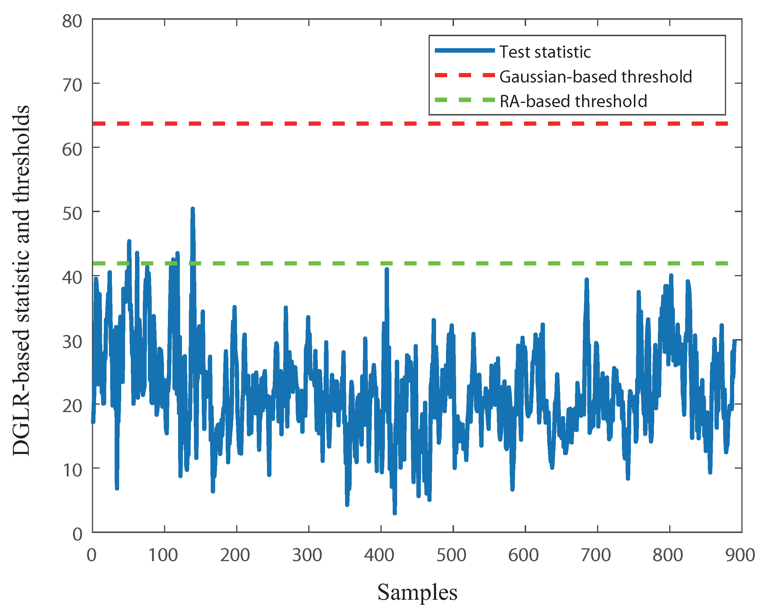
2.2. Randomized Algorithm-Based Threshold Setting

The randomized method has been widely used to the analysis and design of a robust control system [35,36]. Recently, this method has been used for threshold setting for the non-Gaussian process because it is independent of the probability distribution [28]. This successful application can be attributed to the iterative update of the threshold by means of the estimation of false alarm rate (FAR). The basic idea behind is that the required threshold should guarantee a desired false alarm rate, which is predefined. Let $J_{th}$, $p_{FAR}$ and ${\widehat{p}}_{FAR}$ be the threshold, allow FAR and the estimated FAR, respectively A lowest threshold which is satisfied with the given false alarm rate is obtained by the following Algorithm 1 from [28].

Algorithm 1: Threshold-setting

Given allowed $\mathrm{FAR}\in (0,1)$ and $\delta \in (0,1)$, let $ϵ>0$ be some constant satisfying $$\mathrm{FAR}-ϵ>0$$  and $\mathrm{\Delta }>0$ be the iteration tolerance. S1: Set $J_{th}=J_0(>0)$; S2: Choose integer N according to the one-sided Chernoff inequality with $ϵ\in (0,1)$, $\delta \in (0,1)$ $$N\ge \frac{1}{2{ϵ}^2}log\frac{1}{\delta }$$ (9) S3: Estimate FAR using the method given in [37]; S4: If ${\widehat{p}}_{FAR}\le p_{FAR}-ϵ$ then return $J_{th}$ and exit; S5: Else $J_{th}=J_{th}+\mathrm{\Delta }$ go to Step 3.

As given in Theorem 1 in [28], for a sufficiently small $\mathrm{\Delta }$, the estimated threshold satisfies $J_{th,min}\le J_{th}\le J_{th,min}+\mathrm{\Delta }$ with $J_{th,min}$ the lowest threshold. Since $\mathrm{\Delta }$ is sufficiently small, the estimated threshold approaches the lower threshold, i.e., $J_{th}\approx J_{th,min}$.

3. The Proposed Method

In this section, a DGLR-based fault detection method is proposed for non-Gaussian dynamic processes. Firstly, a DGLR-based test statistic is built for detection purposes. Then, it is well known in probability theory that the complete information of a Gaussian distribution can be described by the mean value and the covariance. Therefore, if the measured variable $\mathbf{y}$ follows a Gaussian distribution, the threshold setting can be achieved using the standard distribution table. However, in a non-Gaussian case, the distribution of the test statistics inevitably deviates from the standard distribution, e.g., ${\chi }^2$ distribution. In this case, the threshold, which is set based on Gaussian assumption, will decrease the detection performance, e.g., lower detection rate or higher false alarms. An alternative solution to this problem is to set an appropriate threshold. Therefore, in Section 3.1, the DGLR method is integrate with the RA-based threshold-setting algorithm for the purpose of fault detection of non-Gaussian processes.

3.1. DGLR with RA-Based Threshold Setting Algorithm

In the DGLR-based fault detection method, the solution of fault detection problem consists of two procedures:

• Off-line training. Using the stacking data to identify the unknown parameters, i.e., the mean value $\mathrm{E}\left(\mathbf{y}\right)$ and the covariance matrix $\mathbf{\Sigma }$;
• On-line implementation. Detecting faults with on-line data.

In the first procedure, with N recorded data available, the data can be augmented and stacked in the following manner:

$$\mathbf{y}=\left[\begin{array}{cccc}{y}_k^T& y_{k-1}^T& \cdots & y_{k-N}^T\\ y_{k+1}^T& y_k^T& \cdots & y_{k-N+1}^T\\ ⋮& ⋮& ⋮& ⋮\\ y_{k+p}^T& y_{k+p-1}^T& \cdots & y_{k+p-N}^T\end{array}\right]$$

(10)

where $y_k^T$ denotes the recorded data at time k, and $p+1$ represents the number of samples. The mean value $\mathrm{E}\left(\mathbf{y}\right)$ and the covariance matrix $\mathbf{\Sigma }$ can be estimated according to Equations (7) and (8), respectively. For on-line implementation, first, we collect on-line measurement data ${\mathbf{y}}_{k+i}={[y_{k+i},y_{k+i+1},\dots ,y_{k+i+p}]}^T,i=1,\dots ,n$, and then calculate

$${\overline{\mathbf{y}}}_n=\frac{1}{n}\sum _{i=1}^n{\mathbf{y}}_{k+i},\mathrm{\Delta }\overline{\mathbf{y}}={\overline{\mathbf{y}}}_n-\mathrm{E}\left(\mathbf{y}\right)$$

(11)

For fault detection purposes, a test statistic in a maximum likelihood ratio-like form can be used as

$$J_{DGLR}=n\left(\mathrm{\Delta }{\overline{\mathbf{y}}}^T{\widehat{\mathrm{\Sigma }}}^{-1}\mathrm{\Delta }\overline{\mathbf{y}}\right)$$

(12)

By summarizing the previous analysis, an extension of DGLR using RA-based threshold setting is proposed to detect underlying faults subject to non-Gaussian processes. The step-by-step procedure of the DGLR with RA-based threshold setting algorithm is illustrated in Algorithm 2.

Algorithm 2: DGLR-based fault detection method with RA-based threshold setting.

Off-line training S1: Computation of $$\mathrm{E}\left(\mathbf{y}\right)=\frac{1}{N}\sum _{i=1}^N{\mathbf{y}}_i,\widehat{\mathrm{\Sigma }}=\frac{1}{N-1}\sum _{i=1}^N({\mathbf{y}}_i-\mathrm{E}\left(\mathbf{y}\right)){({\mathbf{y}}_i-\mathrm{E}\left(\mathbf{y}\right))}^T$$ S2: Determine the corresponding thresholds $J_{th,ng}$ using Algorithm 1 with a given significance level $\alpha$, in which the statistic, $J_{DGLR}$ is estimated according to Equation (12); On-line implementation S3: Collect real-time measurement ${\mathbf{y}}_{k+i},i=1,\dots ,n$ and calculate $${\overline{\mathbf{y}}}_n=\frac{1}{n}\sum _{i=1}^n{\mathbf{y}}_{k+i},\mathrm{\Delta }\overline{\mathbf{y}}={\overline{\mathbf{y}}}_n-\mathrm{E}\left(\mathbf{y}\right)$$ S4: Build test statistic $$J_{DGLR}=n\left(\mathrm{\Delta }{\overline{\mathbf{y}}}^T{\widehat{\mathrm{\Sigma }}}^{-1}\mathrm{\Delta }\overline{\mathbf{y}}\right)$$ S5: Check the decision logic: $$\left\{\begin{array}{c}{J}_{DGLR}>J_{th,ng}\Rightarrow \mathrm{faulty}\hfill \\ J_{DGLR}\le J_{th,ng}\Rightarrow \mathrm{fault}-\mathrm{free}.\hfill \end{array}\right.$$

Remark 1.

The extension of PCA-based, DPCA-based, and PCA-based GLR fault detection methods with RA technique can be achieved according to the procedures in Algorithm 2. Hence, they are not presented in this paper.

3.2. Comparison among GLR-Based, DGLR-Based, PCA-Based, DPCA-Based, and PCA-Based GLR Fault Detection Methods

Considering the applications of PCA-based, DPCA-based, and PCA-based GLR fault detection methods, in this subsection, we briefly discuss the relationship among the three fault detection methods with the GLR-based one to distinguish their scope.

In practice, the direct application of the DGLR-based method may be unavailable due to numerical reasons, e.g., the invertibility of the estimated covariance matrix. This fact leads to the application of PCA-based methods, in which the SVD (singular value decomposition) of the estimated covariance matrix is the core. The principle of DPCA is similar to that of PCA, the following introduces the basic PCA technique [5]:

$$\widehat{\mathbf{\Sigma }}=\mathbf{P}\mathbf{\Lambda }{\mathbf{P}}^T=\left[{\mathbf{P}}_{pc}{\mathbf{P}}_{res}\right]\left[\begin{array}{cc}{\mathbf{\Lambda }}_{pc}& 0\\ 0& {\mathbf{\Lambda }}_{res}\end{array}\right]\left[\begin{array}{c}{\mathbf{P}}_{pc}^{\mathrm{T}}\\ {\mathbf{P}}_{res}^{\mathrm{T}}\end{array}\right]$$

where ${\mathbf{P}}_{pc}=\left[{\mathbf{p}}_1,\dots ,{\mathbf{p}}_{\gamma }\right]\in {\mathcal{R}}^{m\times \gamma }$ and ${\mathbf{P}}_{res}=\left[{\mathbf{p}}_{\gamma +1},\dots ,{\mathbf{p}}_m\right]\in {\mathcal{R}}^{m\times (m-\gamma )}$ consist of the loading vectors, known as the principal components and residual components, respectively; $\gamma$ represents the number of principal components, ${\mathbf{\Lambda }}_{pc}=\mathrm{diag}\left({\lambda }_1,\dots ,{\lambda }_{\gamma }\right)$ and ${\mathbf{\Lambda }}_{res}=\mathrm{diag}\left({\lambda }_{\gamma +1},\dots ,{\lambda }_m\right)$ contain the corresponding eigenvalues, satisfying ${\gamma }_1\ge \dots \ge {\lambda }_{\gamma }>>{\lambda }_{\gamma +1}\ge \dots {\lambda }_m$.

For fault detection, the Hotelling’s test statistic can be calculated with a single, on-line measurement

$$\begin{array}{cc}\hfill J_{PCA}& ={(\mathbf{y}-\mathrm{E}\left(\mathbf{y}\right))}^{\mathrm{T}}{\mathbf{P}}_{pc}{\mathbf{\Lambda }}_{pc}^{-1}{\mathbf{P}}_{pc}^{\mathrm{T}}(\mathbf{y}-\mathrm{E}\left(\mathbf{y}\right))\hfill \end{array}$$

(13)

From the calculation formula of two test statistics, it is clear that the data normalization plays a central role. It not only provides us with an estimation of the covariance matrix in off-line training, but also delivers the required residual signal for fault detection.

If the principal component $\gamma <m$, then the matrix ${\mathbf{P}}_{pc}\in {\mathcal{R}}^{m\times \gamma }$ is rank deficient, i.e., $\mathrm{rank}\left({\mathbf{P}}_{pc}\right)=\gamma <m$. From the fault detection viewpoint, the matrix ${\mathbf{P}}_{pc}$ is not ‘all pass’ for faults, that is, there exists $\mathbf{f}\ne \mathbf{0}$ such that ${\mathbf{P}}_{pc}^{\mathrm{T}}\mathbf{f}=0$. This situation is caused by the artificial design of rank deficient matrix ${\mathbf{P}}_{pc}$. If the principal component $\gamma$ equals m, then the $J_{PCA}$ statistic reduces to Hotelling’s $T^2$ statistic, that is, when $\gamma =m$

$$\begin{array}{cc}\hfill J_{PCA}& ={(\mathbf{y}-\mathrm{E}\left(\mathbf{y}\right))}^{\mathrm{T}}\mathbf{P}{\mathbf{\Lambda }}^{-1}{\mathbf{P}}^{\mathrm{T}}(\mathbf{y}-\mathrm{E}\left(\mathbf{y}\right))\hfill \\ \hfill & ={(\mathbf{y}-\mathrm{E}\left(\mathbf{y}\right))}^{\mathrm{T}}{\widehat{\mathrm{\Sigma }}}^{-1}(\mathbf{y}-\mathrm{E}\left(\mathbf{y}\right))\hfill \end{array}$$

(14)

As introduced in [5], the test statistic $J_{DGLR}$ in the form (12) is also called Hotelling’s $T^2$ test statistic. It is evident that the test statistic in form (14) is equivalent with the one in (12) under the single on-line measurement case.

It is worthwhile noting that, recently, a PCA-based GLR fault detection method was proposed in [34], in which the PCA technique is only used for establishing the mathematical process model and the GLR test is used to evaluate the residual signal.

Table 1. Comparison between (D)GLR-based, (D)PCA-based and PCA-based GLR fault detection methods.

Method	Application Conditions	Number of Test Statistics	Parameters
GLR(DGLR)-based	${\widehat{\mathbf{\Sigma }}}^{-1}$ is available	$J_{GLR}$ and $J_{DGLR}$	m, n, $\mathrm{E}\left(y\right)$ and $\widehat{\mathbf{\Sigma }}$
PCA(DPCA)-based	${\widehat{\mathbf{\Sigma }}}^{-1}$ is unavailable	$J_{PCA}$ and $J_{DPCA}$	m, $\gamma$, ${\mathbf{P}}_{pc}$, ${\mathbf{P}}_{res}$ $\mathrm{E}\left(y\right)$ and $\widehat{\mathbf{\Sigma }}$
PCA-based GLR	Both cases, in which PCA model is available	$J_{PG}$	m, $\gamma$, ${\mathbf{P}}_{res}$, $\mathrm{E}\left(y\right)$ and $\widehat{\mathbf{\Sigma }}$

presents a comparison between them to clarify their relationship.

Actually, the numerical problem of ${\widehat{\mathrm{\Sigma }}}^{-1}$ is rare due to the presence of process noise and measurement error. Hence, in this paper, we assume that ${\widehat{\mathrm{\Sigma }}}^{-1}$ is available.

Remark 2.

The other use of PCA is for dimensionality reduction purpose. However, for fault detection, dimension reduction is not always crucial [32].

4. Simulated Examples

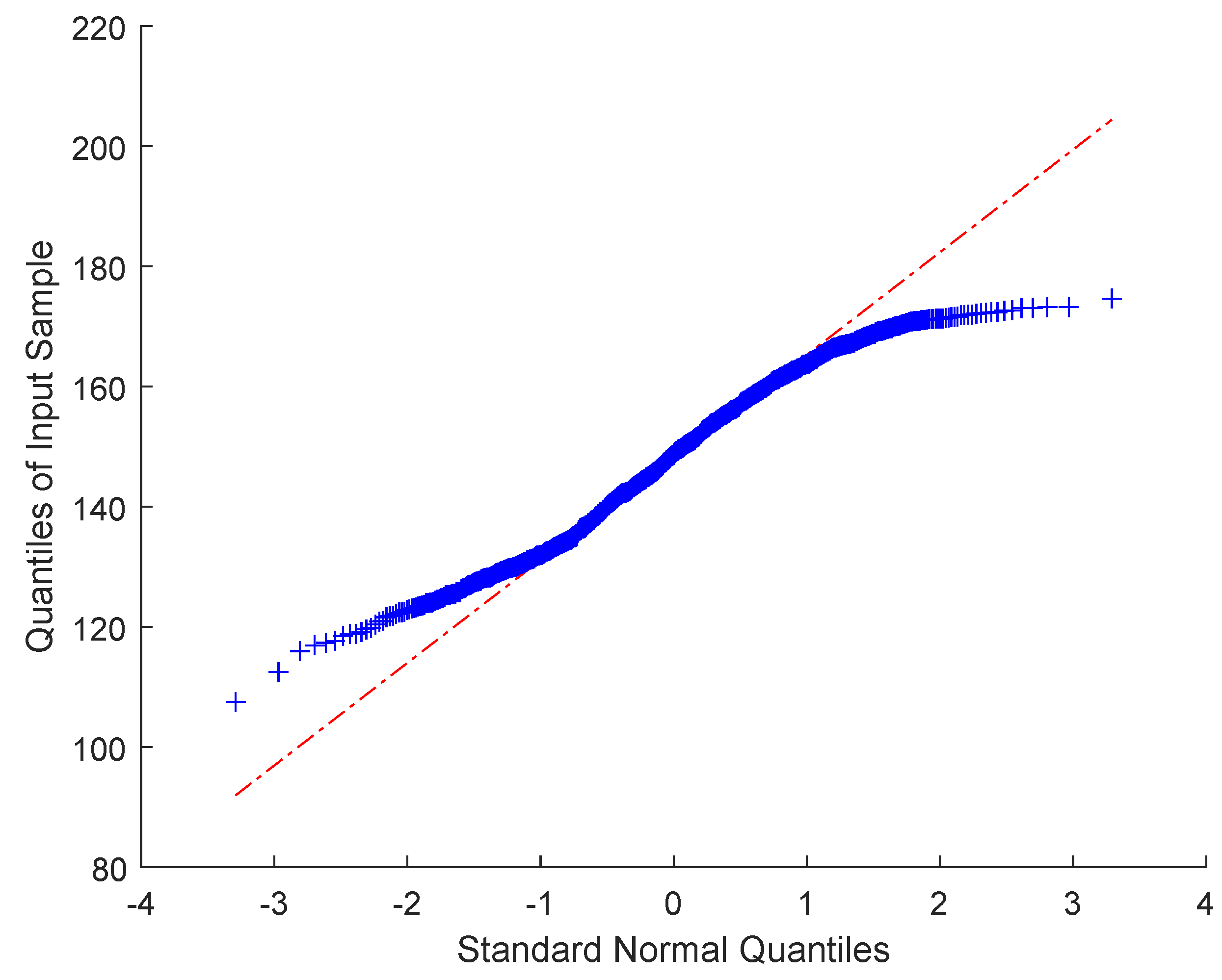
4.1. Fault Detection in Synthetic Data

In this example, a non-Gaussian dynamic process is first simulated by using Matlab. Then, the performance of the GLR-based, DGLR-based, PCA-based, DPCA-based, and PCA-based GLR fault detection methods is assessed through its application to detect faults in synthetic data.

4.1.1. Data Generation

Except for the fact that the noise sources are non-Gaussian, the model for data generation is the same as the one used in [38], which is given as:

$${\mathbf{y}}_k=\mathbf{T}\left(q^{-1}\right){\mathbf{u}}_k+\mathbf{K}\left(q^{-1}\right){\mathbf{d}}_k+{\mathbf{n}}_k+{\mathbf{f}}_{y,k},$$

(15)

where

$$\mathbf{T}\left(q^{-1}\right)=\left[\begin{array}{cccc}\frac{0.05q^{-3}}{1-0.95q^{-1}}& 0& \frac{0.7q^{-3}}{1-0.3q^{-1}}& 0\\ \frac{0.02966q^{-3}}{1-1.627q^{-1}+0.706q^{-2}}& \frac{0.0627q^{-6}}{1-0.937q^{-1}}& 0& 0\\ 0& \frac{0.235q^{-5}}{1-0.765q^{-1}}& \frac{0.5q^{-2}}{1-q^{-1}+0.25q^{-2}}& 0\\ \frac{0.5q^{-5}-0.4875q^{-6}}{1-1.395q^{-1}+0.455q^{-2}}& 0& 0& \frac{0.2q^{-6}}{1-0.8q^{-1}}\end{array}\right]$$

$$\mathbf{K}\left(q^{-1}\right)={\left[\begin{array}{cccc}\frac{1-0.1875q^{-1}}{1-0.9875q^{-1}}\hfill & \frac{1-0.1875q^{-1}}{1-0.9875q^{-1}}\hfill & \frac{1-0.1875q^{-1}}{1-0.9875q^{-1}}\hfill & \frac{1-0.1875q^{-1}}{1-0.9875q^{-1}}\hfill \end{array}\right]}^{\mathrm{T}}$$

${\mathbf{y}}_k$ and ${\mathbf{u}}_k$ are the output and control input vectors, ${\mathbf{n}}_k$ denotes the independent non-Gausian white noise, ${\mathbf{f}}_{y,k}$ is the fault introduced in k-th sensor. The four controllers are given as

$$u_k^i=G_i\left(q^{-1}\right)y_k^i,i=1,2,3,4$$

(16)

where

$$\begin{array}{cc}\hfill & G_1\left(q^{-1}\right)=\frac{-3.2235+3.07q^{-1}}{1-q^{-1}},G_2\left(q^{-1}\right)=\frac{-0.6641+0.625q^{-1}}{1-q^{-1}},\hfill \\ \hfill & G_3\left(q^{-1}\right)=\frac{-0.6991+0.518q^{-1}}{1-q^{-1}},G_4\left(q^{-1}\right)=\frac{-0.444+3.70q^{-1}}{1-q^{-1}}.\hfill \end{array}$$

The above model is used to simulate 1000 fault-free data samples. These data are used to estimate the required parameters for the three fault detection methods. The number of principal components is determined as four by using of the cumulative percent variance method. p is set to be five, which is determined as given in [20]. To validate the detection performance, three faults listed in

Table 2. Faults introduced in process.

Fault IDs	Description	Value of $\mathit{\delta }$
1	$y_{1,i}=y_{1,0}+\delta$	0.2
2	$y_{1,i}=y_{1,0}+\delta t$	0.005
3	$y_{1,i}=y_{1,0}+\delta$	$\mathcal{N}$(0, 0.04)

are introduced in this process.

After identifying the required parameters, one significant problem remaining in the training phase is to set the threshold. For threshold-setting, the sample number $N=2.65\times {10}^4$ is set using Equation (9) for $ϵ=0.01$, $\delta =0.01$. The remaining steps are followed by Algorithm 2. Given a significance level of 0.01,

Table 3. Thresholds of all test statistics.

Method	Test Statistics	RA-Based Threshold	Gaussian-Based Threshold
GLR	$J_{GLR}$	$J_{th,GLR}=13.3011$	20.0901
DGLR	$J_{DGLR}$	$J_{th,DGLR}=22.6015$	32.0001
PCA	$J_{PCA}$	$J_{th,PCA}=9.0010$	13.2775
DPCA	$J_{DPCA}$	$J_{th,DPCA}=4.0105$	4.1991
PCA-based GLR	$J_{PG}$	$J_{th,PG}=10.4016$	13.2775

lists the thresholds used in this work.

In order to demonstrate the advantage of the proposed RA-based threshold setting, the $J_{DGLR}$ test statistic is used as an example. The result of this statistic is shown in Figure 1, where the red line represents the Gaussian assumption-based threshold and the green line represents the RA-based threshold. Figure 1 shows that the $J_{DGLR}$ test statistic is always below the threshold value, which means a zero false alarm rate. Unfortunately, zero FAR will lead to a lower fault detection rate (FDR). From Figure 1, we can see that the RA-based threshold makes the $J_{DGLR}$ statistic approach to a FAR of 0.01, which satisfies the given significance level. Due to the limited space, we only use this statistic as an example. Next, only the RA-based threshold is used for comparison purpose.

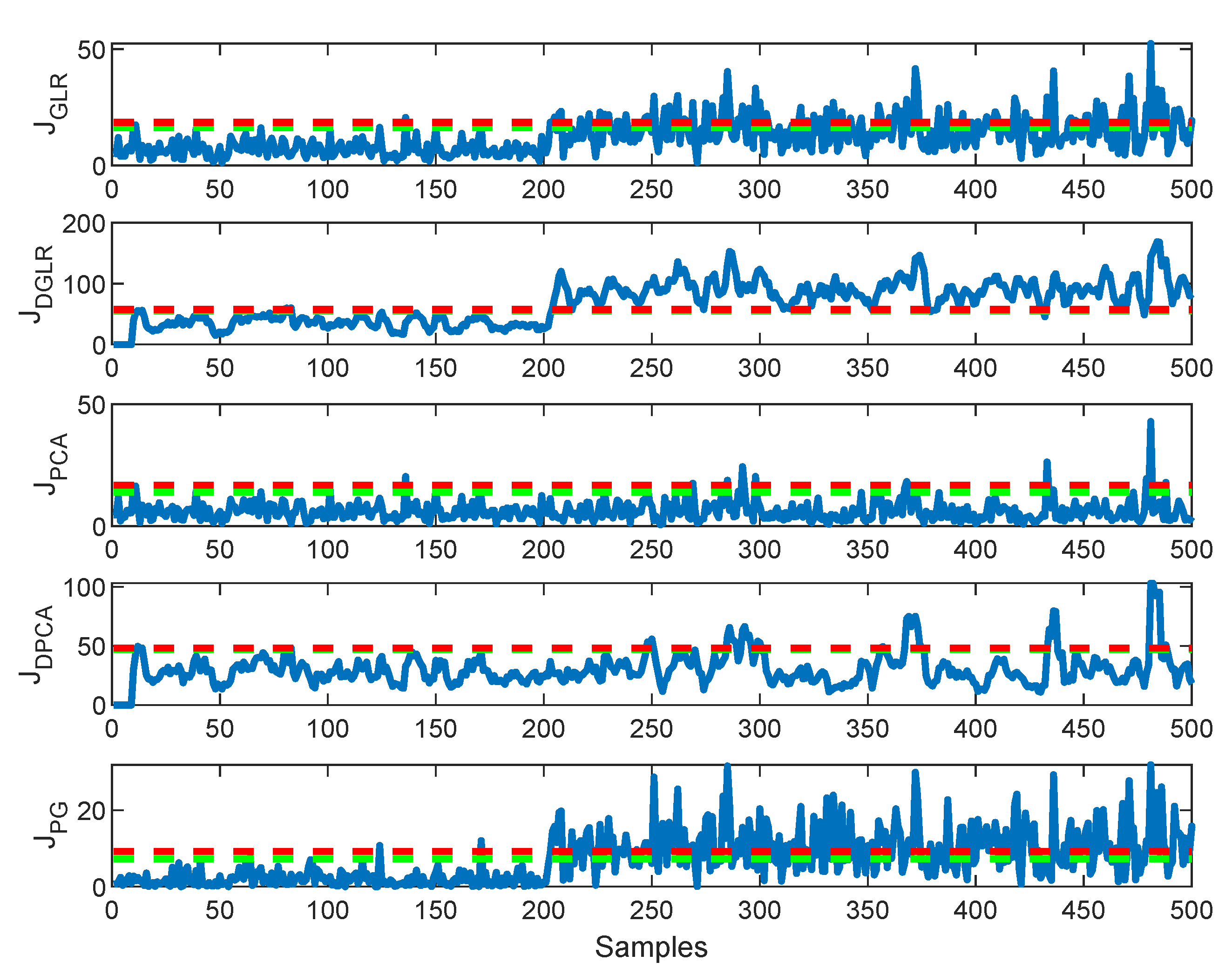
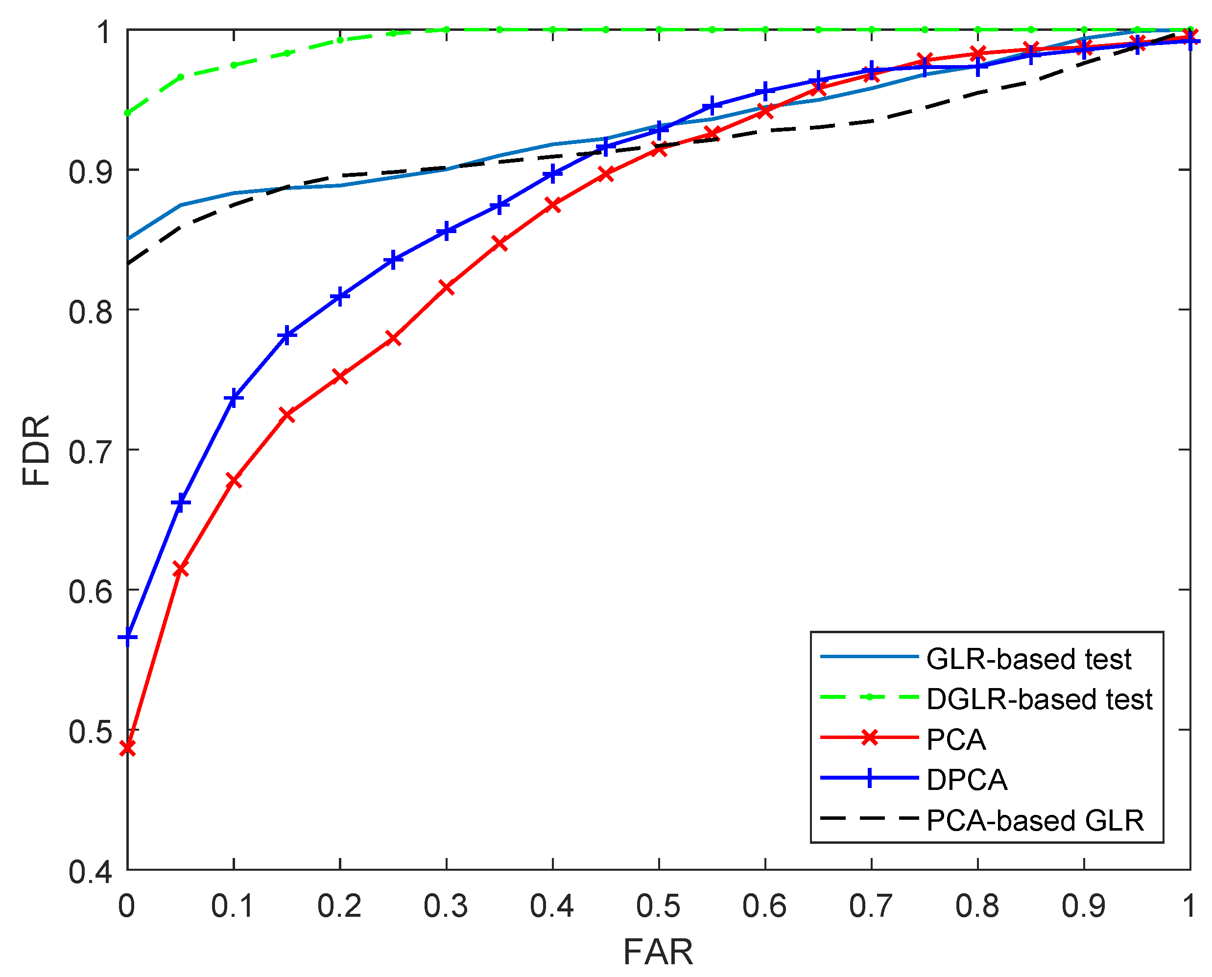
4.1.2. Comparing the Five Methods Using Faulty Data

The testing data set, which is simulated using the same model given in Equation (15), consists of 1000 data samples, which are completely independent from the training data. In this case, the possibility of only a single fault is considered. To assess the abilities of the various fault detection methods, Fault 2 was introduced at the sample of 400. To compare the performances of the GLR-based, DGLR-based, PCA-based, DPCA-based, and PCA-based GLR methods, the receiver operating characteristic (ROC) curves of the five methods are shown in Figure 2, which shows the FDR for different values of the fault alarm rate (FAR). The ROC curves provide a measure to compare the detection accuracy of all test statistics in three methods as well as their sensitivities to variations in the detection thresholds. Figure 2 shows that there is a trade-off between a high FDR and a low FAR. It can be seen that the PCA-based GLR test provides a higher FDR than the conventional PCA-based method. This fact is consistent with the conclusion in [34]. The $J_{GLR}$ statistic of GLR-based method has a similar detection performance as the PCA-based GLR test. Evidently, the DGLR-based method has the highest FDR than the other four test statistics. This clearly shows the advantages of the DGLR-based method over the other methods. Furthermore, the FDR performance of the DGLR-based method can be further improved by choosing the number of p. It should also be kept in mind that a large value of p can lead to a high detection delay. Therefore, there is also a trade-off between FDR and detection delay when determining an appropriate p.

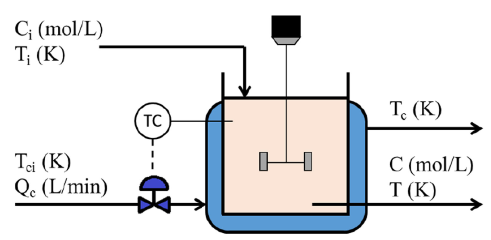
4.2. Fault Detection in CSTR Process

4.2.1. Data Generation

To validate the proposed method, a CSTR process is used with several typical faulty scenarios. CSTR is widely used in chemical processes and the Matlab simulation model used in this study is similar to that used in [39]. The schematic of this CSTR is shown in Figure 3, where the reactor temperature T is controlled by manipulating the coolant flow rate $Q_c$. As can be seen, it consists of three inputs ($C_i$, $T_i$, and $T_{ci}$) and four outputs (C, T, $T_C$, and $Q_c$). The corresponding model is given as follows:

$$\frac{dC}{dt}=\frac{Q}{V}\left(C_i-C\right)-akC+{\nu }_1$$

(17)

$$\frac{dT}{dt}=\frac{Q}{V}\left(T_i-T\right)-a\frac{\left(\mathrm{\Delta }{H}_r\right)kC}{\rho C_p}-b\frac{UA}{\rho C_{p}V}\left(T-T_c\right)+{\nu }_2$$

(18)

$$\frac{d{T}_c}{dt}=\frac{Q_c}{V_c}\left(T_{ci}-T_c\right)+b\frac{UA}{{\rho }_c{C}_{pc}{V}_c}\left(T-T_c\right)+{\nu }_3$$

(19)

where $v_i$ represents process noise, k is an Arrhenius-type rate constant, $k=k_{0}exp\left(\frac{-E}{RT}\right)$. The parameters in the above model are listed in

Table 4. Constant parameters in CSTR model.

Parameter	Description	100.0	Unit
Q	Inlet flow rate	150.0	L/min
V	Tank volume	10.0	L
$V_c$	Jacket volume	0.7	L
$\mathrm{\Delta }{H}_r$	Heat of reaction	$-2.0\times {10}^5$	cal/mol
UA	Heat transfer coefficient	$7.0\times {10}^5$	cal/min/K
$k_0$	Pre-exponential factor to k	$7.2\times {10}^{10}$	min−1
$ER$	Activation energy	$1.0\times {10}^4$	K
$\rho ,{\rho }_c$	Fluid density	1000	g/L
$C_p,C_{pc}$	Fluid heat capacity	1.0	cal/g/K

. Five typical faults are used to validate the proposed fault detection method, which have been descripted and listed in

Table 5. Brief description of typical CSTR faults.

Fault IDs	Description of Faults	Value of $\mathit{\delta }$
1	$b=b_{0}exp(-\delta t)$	0.001
2	$a=a_0+\delta$	1.4
3	$T_c=T_{c,0}+\delta$	0.7
4	$C=C_0+\delta$	0.005
5	$Q_c=Q_{c,0}+\delta$	5

. $b_0$, $a_0$, $T_{c,0}$, $C_0$, and $Q_{c,0}$ in table are nominal values. Fault 1 and Fault 2 represent catalyst decay and heat transfer fouling, and Faults 3–5 are the sensor faults on each of the three measured variables.

In existing literature, there are several ways to check the non-Gaussianity. Among them, the probability plot of the variables is the most commonly used. We plot the quantiles of the A phase of converter current as an example. Figure 4 shows the distribution of the variable, where ‘+’ denotes the sample and the dotted line shows the locus of zero-mean samples which are normally distributed. It can be seen that the samples do not match the zero-mean normal distribution, that is, the samples from the example system obey the non-Gaussian distribution.

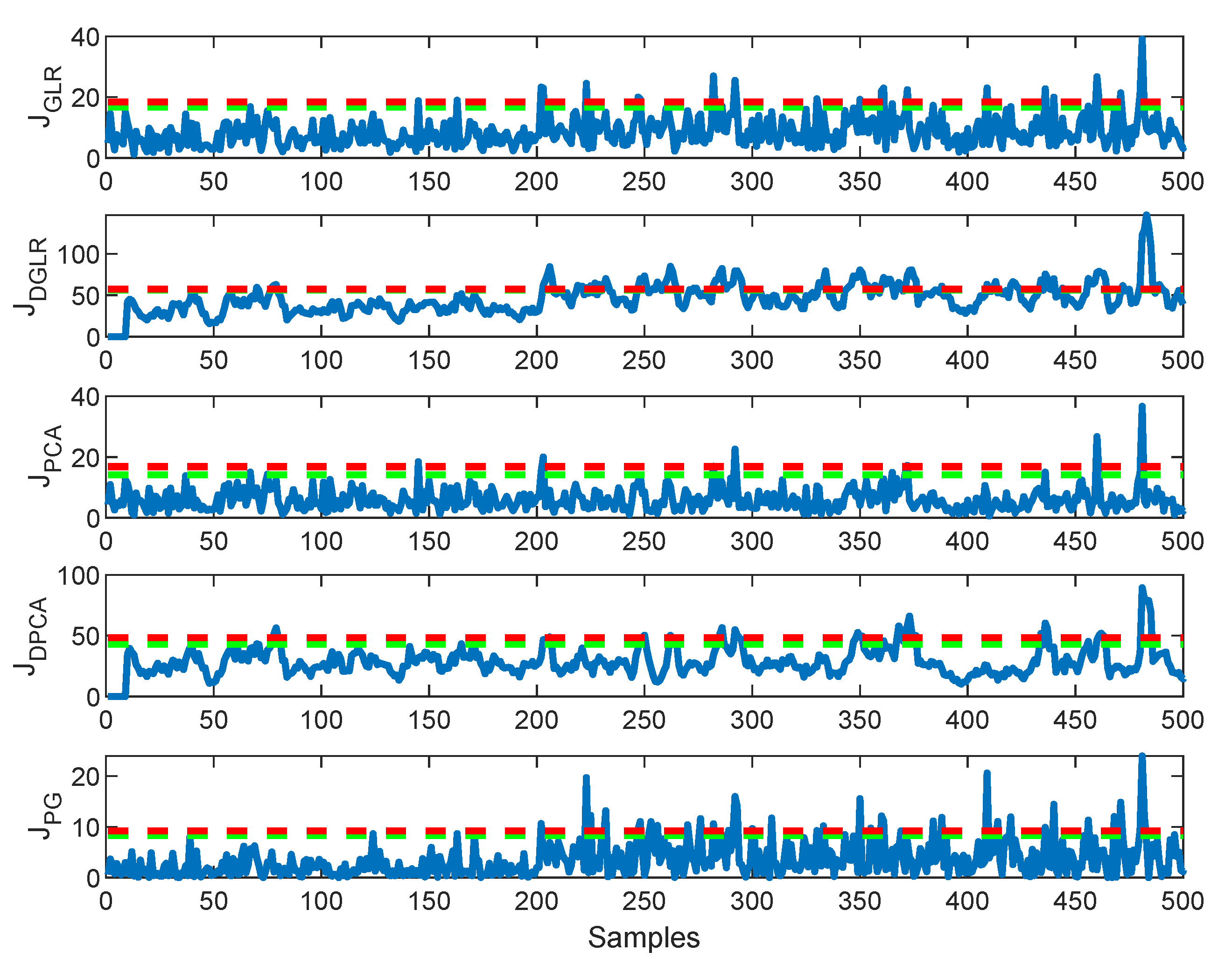
4.2.2. Comparing the Five Methods Using Faulty Data

The CSTR data consist of two blocks: the training and test data blocks. The normal operating data will be referred to as the training data. Then, parameters $\mathrm{E}\left(\mathbf{y}\right)$ and $\widehat{\mathbf{\Sigma }}$ used in the proposed method are estimated from the training data. After obtaining the necessary parameters, one remaining issue in the training phase is to determine an appropriate threshold. For threshold-setting, the sample number $N=2.65\times {10}^4$ is chosen by means of Equation (9) for $ϵ=0.01$, $\delta =0.01$. Hence, the thresholds used in this work are determined as $J_{th,GLR}=$ 16.20, $J_{th,DGLR}=$ 56.60, $J_{th,PCA}=$ 15.40, $J_{th,DPCA}=$ 50.20 and $J_{PG}=$ 66.01 with a significance level of 0.01. The number of principal components and time lag p are set to be six and five, respectively. The total samples of each operation run in the test data block are 500 and the various faults are introduced only at sample 200. This means that for each of the faults, the process is fault-free for the first 200 samples before the system becomes abnormal at the introduction of the fault.

To demonstrate the effectiveness of the proposed method, the monitoring performance will be discussed. The detection sensitivity of a fault detection method is commonly quantified by calculating the FDR, which will be used for discussing the detection sensitivity of the proposed methods. The response of the fault detection method is commonly represented by the detection delay (DD), which is the time period it takes to detect a fault after occurrence of the fault. As the desired FAR is given for threshold-setting, the two indicators, FDR and DD, are used to assess the detection performance of fault detection methods. From the result discussion of Figure 2, the detection performance of the proposed method is compared with the GLR-based, PCA-based, DPCA-based, and PCA-GLR-based methods by using all faults described above. The superiority of the test statistic $J_{DGLR}$ over the other test statistics considered in this paper is shown in

Table 6. Detection results with respect to FDR.

Fault IDs	${\mathit{J}}_{\mathit{GLR}}$	${\mathit{J}}_{\mathit{DGLR}}$	${\mathit{J}}_{\mathit{PCA}}$	${\mathit{J}}_{\mathit{DPCA}}$	${\mathit{J}}_{\mathit{PG}}$
1	79.74%	85.38%	16.39%	61.16%	86.49%
2	99.35%	96.75%	99.35%	96.76%	99.35%
3	54.34%	95.77%	8.03%	15.85%	85.53%
4	9.03%	48.37%	11.57%	50.48%	20.57%
5	6.75%	36.36%	5.46%	14.88%	21.54%

with respect to FDR. Due to the non-Gaussian characteristic, the test statistic $J_{DGLR}$ with RA achieves the better performance with the higher FDR value than all faults compared. Detection delays of all test statistics are presented in

Table 7. Detection results with respect to DD.

Fault IDs	${\mathit{J}}_{\mathit{GLR}}$	${\mathit{J}}_{\mathit{DGLR}}$	${\mathit{J}}_{\mathit{PCA}}$	${\mathit{J}}_{\mathit{DPCA}}$	${\mathit{J}}_{\mathit{PG}}$
1	42	34	16	47	47
2	2	2	2	2	2
3	2	3	27	47	47
4	18	4	18	4	4
5	1	2	1	2	2

. The unit of DD is the same as the sample interval. As shown in Table 7, the $J_{DGLR}$ with RA test statistics is able to detect most of these faults earlier than the other ones. This point alos demonstrates the advantage of the test statistics $J_{DGLR}$.

For demonstrating the advantages of DGLR with the RA approach, the detection results of both methods for Faults 3 and 5 are shown in Figure 5 and Figure 6, respectively. The solid line represents the test statistic, the red line is the threshold based on a Gaussian assumption, and the blue line means the threshold based on the RA approach. In both figures, from top to bottom, there are $J_{GLR}$ test statistics of the GLR-based method, $J_{DGLR}$ of the DGLR-based method, $J_{PCA}$ of the PCA-based method, $J_{DPCA}$ of the DPCA-based method, and $J_{PG}$ of the PCA-based GLR method, respectively. FDRs of the GLR-based, DGLR-based, PCA-based, DPCA-based, and PCA-based GLR methods are 6.7%, 36.3%, 5.4%, 14.87%, and 21.54%, respectively. DDs of the GLR-based, DGLR-based, PCA-based, DPCA-based, and PCA-based GLR methods are 1, 2, 1, 2, and 2 min, respectively. All figures clearly show that all test statistics are able to detect the faults. In addition, the test statistics with the RA approach result in a higher FDR and smaller detection delay than the standard test statistics without RA. It should be noted that the performances of $J_{DGLR}$ test statistic with respect to FDR and DD are better than its companions in both faulty cases.

5. Conclusions

In this work, a DGLR-based method has been proposed for non-Gaussian dynamic processes, which combines the standard GLR method and the RA approach to iteratively learn the suitable threshold, which releases the assumption of Gaussian distributed variables. Furthermore, the DGLR-based approach has been compared with GLR-based, PCA-based, DPCA-based, and PCA-based GLR fault detection approaches to clarify the application scope of these methods. The major difference between them lies in the inverse of the estimated covariance matrix. In addition, the detection performance of the DGLR-based method has been compared with the aforementioned methods using a numerical simulation of a non-Gaussian process and the CSTR process. The comparison results show that the DGLR-based approach is better than the other methods. For instance, the average FDRs of the GLR-based, DGLR-based, PCA-based, DPCA-based, and PCA-based GLR approaches are 49.84%, 72.52%, 28.16%, 47.82%, 62.69% in CSTR process. The average DDs of the GLR-based, DGLR-based, PCA-based, DPCA-based, and PCA-based GLR methods are 13, 9, 12.8, 20.4, and 20.4 min in CSTR process. The $J_{DGLR}$ test statistics of the DGLR-based method shows the best detection performance compared with all other test statistics considered in this paper. Because the detection performance could be affected by kinds of factors, the robustness of the proposed method will be validated by using real data collected in industrial processes in the future.

References

1. Maleki, M.R.; Amiri, A.; Castagliola, P. Measurement errors in statistical process monitoring: A literature review. Comput. Ind. Eng. 2017, 103, 316–329. [Google Scholar] [CrossRef]
2. Zhao, C.; Chen, J.; Jing, H. Condition-Driven Data Analytics and Monitoring for Wide-Range Nonstationary and Transient Continuous Processes. IEEE Trans. Autom. Sci. Eng. 2021, 18, 1563–1574. [Google Scholar] [CrossRef]
3. He, Z.; Chen, Z.; Zhou, H.; Wang, D.; Xing, Y.; Wang, J. A visualization approach for unknown fault diagnosis. Chemom. Intell. Lab. Syst. 2018, 172, 80–89. [Google Scholar] [CrossRef]
4. Huang, K.; Zhang, L.; Yang, C.; Gui, W.; Hu, S. Unified Stationary and Nonstationary Data Representation for Process Monitoring in IIoT. IEEE Trans. Instrum. Meas. 2022, 71, 1–12. [Google Scholar] [CrossRef]
5. Ding, S.X. Data-Driven Design of Fault Diagnosis and Fault-Tolerant Control Systems; Springer: London, UK, 2014. [Google Scholar]
6. Luo, H.; Yang, X.; Krueger, M.; Ding, S.; Peng, K. A plug-and- play monitoring and control architecture for disturbance compensation in rolling mills. IEEE/ASME Trans. Mechatron. 2018, 23, 200–210. [Google Scholar] [CrossRef]
7. Basseville, M.; Nikiforov, I. Detection of Abrupt Changes: Theory and Application; Prentice-Hall: New York, NY, USA, 1993. [Google Scholar]
8. Gao, Z.W.; Cecati, C.; Ding, S.X. A Survey of Fault Diagnosis and Fault-Tolerant Techniques, Part I: Fault Diagnosis with Model-Based and Signal-Based Approaches. IEEE Trans. Ind. Electron. 2015, 62, 3757–3767. [Google Scholar] [CrossRef] [Green Version]
9. Chaouch, H.; Charfeddine, S.; Ben Aoun, S.; Jerbi, H.; Leiva, V. Multiscale monitoring using machine learning methods: New methodology and an industrial application to a photovoltaic system. Mathematics 2022, 10, 890. [Google Scholar] [CrossRef]
10. Chen, H.; Jiang, B.; Lu, N.; Mao, Z. Deep PCA Based Real-Time Incipient Fault Detection and Diagnosis Methodology for Electrical Drive in High-Speed Trains. IEEE Trans. Veh. Technol. 2018, 67, 4819–4830. [Google Scholar] [CrossRef]
11. Cao, Y.; Yuan, X.; Wang, Y.; Gui, W. Hierarchical hybrid distributed PCA for plant-wide monitoring of chemical processes. Control. Eng. Pract. 2021, 111, 104784. [Google Scholar] [CrossRef]
12. Liu, Q.; Kong, D.; Qin, S.J.; Xu, Q. Map-Reduce Decentralized PCA for Big Data Monitoring and Diagnosis of Faults in High-Speed Train Bearings. IFAC-PapersOnLine 2018, 51, 144–149. [Google Scholar] [CrossRef]
13. Peng, K.X.; Zhang, K.; Li, G.; Zhou, D.H. Contribution rate plot for nonlinear quality-related fault diagnosis with application to the hot strip mill process. Control Eng. Pract. 2013, 21, 360–369. [Google Scholar] [CrossRef]
14. Zhang, K.; Hao, H.Y.; Chen, Z.W.; Ding, S.X.; Peng, K.X. A Comparison and evaluation of key performance indicator-based multivariate statistics process monitoring approaches. J. Process. Control 2015, 33, 112–126. [Google Scholar] [CrossRef]
15. Yin, S.; Wang, G.; Gao, H. Data-driven process monitoring based on modified orthogonal projections to latent Structures. IEEE Trans. Control. Syst. Technol. 2016, 24, 1480–1487. [Google Scholar] [CrossRef]
16. Chen, Z.W.; Ding, S.X.; Zhang, K.; Li, Z.B.; Hu, Z.K. Canonical correlation analysis-based fault detection methods with application to alumina evaporation process. Control Eng. Pract. 2016, 46, 51–58. [Google Scholar] [CrossRef]
17. Chen, Z.; Yang, C.; Peng, T.; Dan, H.; Li, C.; Gui, W. A Cumulative Canonical Correlation Analysis-Based Sensor Precision Degradation Detection Method. IEEE Trans. Ind. Electron. 2019, 66, 6321–6330. [Google Scholar] [CrossRef]
18. Chen, H.; Li, L.; Shang, C.; Huang, B. Fault Detection for Nonlinear Dynamic Systems with Consideration of Modeling Errors: A Data-Driven Approach. IEEE Trans. Cybern. 2022, 1–11. [Google Scholar] [CrossRef]
19. Ge, Z.Q.; Song, Z.H.; Gao, F.R. Review of recent research on data-based process monitoring. Ind. Eng. Chem. Res. 2013, 52, 3543–3562. [Google Scholar] [CrossRef]
20. Ku, W.F.; Storer, R.H.; Georgakis, C. Disturbance detection and isolation by dynamic principal component analysis. Chemom. Intell. Lab. Syst. 1995, 30, 179–196. [Google Scholar] [CrossRef]
21. Wang, X.; Kruger, U.; Irwin, G.W. Process Monitoring Approach Using Fast Moving Window PCA. Ind. Eng. Chem. Res. 2005, 44, 5691–5702. [Google Scholar] [CrossRef]
22. Chen, Q.; Wynne, R.; Goulding, P.; Sandoz, D. The application of principal component analysis and kernel density estimation to enhance process monitoring. Control Eng. Pract. 2000, 8, 531–543. [Google Scholar] [CrossRef]
23. Zhang, Q.; Basseville, M. Statistical detection and isolation of additive faults in linear time-varying systems. Automatica 2014, 50, 2527–2538. [Google Scholar] [CrossRef]
24. Kini, K.R.; Madakyaru, M. Monitoring multivariate process using improved Independent component analysis-generalized likelihood ratio strategy. IFAC Pap. 2020, 53, 392–397. [Google Scholar] [CrossRef]
25. Tang, M.; Yang, C.; Gui, W. Fault detection based on cost-sensitive support vector machine for alumina evaporation process. Control Eng. China 2011, 18, 645–649. [Google Scholar]
26. Jiang, Q.; Yan, X.; Lv, Z.; Guo, M. Independent component analysis-based non-Gaussian process monitoring with preselecting optimal components and support vector data description. Int. J. Prod. Res. 2014, 52, 3273–3286. [Google Scholar] [CrossRef]
27. He, Q.P.; Wang, J. Statistics pattern analysis: A new process monitoring framework and its application to semiconductor batch processes. AIChE J. 2011, 57, 107–121. [Google Scholar] [CrossRef]
28. Chen, Z.W.; Ding, S.X.; Peng, T.; Yang, C.H.; Gui, W.H. Fault Detection for Non-Gaussian Processes Using Generalized Canonical Correlation Analysis and Randomized Algorithms. IEEE Trans. Ind. Electron. 2018, 65, 1559–1567. [Google Scholar] [CrossRef]
29. Bishop, C.M. Pattern Recognition and Machine Learning (Information Science and Statistics); Springer: Secaucus, NJ, USA, 2006. [Google Scholar]
30. Chen, T.; Morris, J.; Martin, E. Probability density estimation via an infinite Gaussian mixture model: Application to statistical process monitoring. J. R. Stat. Soc. Ser. C (Appl. Stat.) 2006, 55, 699–715. [Google Scholar] [CrossRef] [Green Version]
31. Odiowei, P.; Cao, Y. Nonlinear dynamic process monitoring using canonical variate analysis and kernel density estimations. IEEE Trans. Ind. Inform. 2010, 6, 36–45. [Google Scholar] [CrossRef] [Green Version]
32. Gonzalez, R.; Huang, B.; Lau, E. Process monitoring using kernel density estimation and Bayesian networking with an industrial case study. ISA Trans. 2015, 58, 330–347. [Google Scholar] [CrossRef]
33. Tschumitschew, K.; Klawonn, F. Incremental quantile estimation. Evol. Syst. 2010, 1, 253–264. [Google Scholar] [CrossRef]
34. Harrou, F.; Nounou, M.N.; Nounou, H.N.; Madakyaru, M. Statistical fault detection using PCA-based GLR hypothesis testing. J. Loss Prev. Process. Ind. 2013, 26, 129–139. [Google Scholar] [CrossRef]
35. Chamanbaz, M.; Dabbene, F.; Tempo, R.; Venkataramanan, V.; Wang, Q.G. Sequential randomized algorithms for convex optimization in the presence of uncertainty. IEEE Trans. Autom. Control 2016, 61, 2565–2571. [Google Scholar] [CrossRef] [Green Version]
36. Faradonbeh, M.K.S.; Tewari, A.; Michailidis, G. Randomized algorithms for data-drivn stabilization of stochastic linear systems. In Proceedings of the 2019 IEEE Data Science Workshop (DSW), Minneapolis, MN, USA, 2–5 June 2019; pp. 170–174. [Google Scholar]
37. Chen, Z.W. Data-Driven Fault Detection for Industrial Processes: Canonical Correlation Analysis and Projection based Methods. Ph.D. Thesis, University of Duisburg-Essen, Duisburg, Germany, 2016. [Google Scholar]
38. McNabb, C.A.; Qin, S.J. Fault diagnosis in the feedback-invariant subspace of closed-loop systems. Ind. Eng. Chem. Res. 2005, 44, 2359–2368. [Google Scholar] [CrossRef]
39. Pilario, K.E.S.; Cao, Y. Canonical variate dissimilarity analysis for process incipient fault detection. IEEE Trans. Ind. Inform. 2018, 14, 5308–5315. [Google Scholar] [CrossRef] [Green Version]
Figure 1. Detection results of DGLR in fault-free case.
Symmetry 14 01332 g001
Figure 2. ROC curves of the five fault detection methods.
Symmetry 14 01332 g002
Figure 3. The schematic diagram of CSTR.
Symmetry 14 01332 g003
Figure 4. Probability distribution of the variable.
Symmetry 14 01332 g004
Figure 5. Detection results of Fault 3.
Symmetry 14 01332 g005
Figure 6. Detection results of Fault 5.
Symmetry 14 01332 g006