Abstract
Bin packing is a typical optimization problem with many real-world application scenarios. In the online bin packing problem, a sequence of items is revealed one at a time, and each item must be packed into a bin immediately after its arrival. Inspired by duality in optimization, we proposed pattern-based adaptive heuristics for the online bin packing problem. The idea is to predict the distribution of items based on packed items, and to apply this information in packing future arrival items in order to handle uncertainty in online bin packing. A pattern in bin packing is a combination of items that can be packed into a single bin. Patterns selected according to past items are adopted and periodically updated in scheduling future items in the algorithm. Symmetry in patterns and the stability of patterns in the online bin packing problem are discussed. We have implemented the algorithm and compared it with the Best-Fit in a series of experiments with various distribution of items to show its effectiveness.
1. Introduction
Combinatorial optimisation problems have extensive applications in many real-world applications. However, most of them are NP-hard and finding the optimal solutions becomes computationally prohibitive because of combinatorial explosion. The existing approaches to these problems can broadly be classified into analytical-model-driven methods and data-driven methods. Analytical-model-driven methods focus on the analytical properties of the mathematical model but suffer from robustness issues over uncertainties from the input data. Heuristic algorithms generally compute feasible solutions with low computational complexity, not optimum. Data-driven methods often formulate the combinatorial problems as online optimization problems and try to tackle the problem in a generative fashion. One of the main drawbacks of the these data-driven methods is their inability to efficiently exploit the core structures and properties of the problem. More specifically, existing data-driven methods primarily focus on the objectives to be optimized, but neglect various complex inter-dependencies among the decision variables in the form of constraints. This can be illustrated with the following example for the bin packing problem.
A one-dimensional bin packing problem aims to use the minimum number of bins of identical size to pack a set of items of different sizes. In its offline version, the sizes of the items are given prior to the packing. Let B denote the capacity of the bins to be used. The problem is to pack all the items of n types, with each item type i having a size and quantity . Let be a binary variable to indicate whether bin j is used in a solution () or not (). Let be the number of times item type i is packed in bin j. The problem can be formulated as follows:
where U is the maximal number of possible bins available to use.
In an online bin packing problem, we consider an infinite sequence of items without prior knowledge of their sizes. Each item needs to be packed at the time of arrival. Heuristic algorithms are commonly used to solve this kind of problem with uncertainty, since optimal solutions are impossible to acquire.
If the distribution of items in an online BPP is known, it is possible to acquire near-optimal solutions by utilizing such knowledge. A straightforward idea is to compute the distribution of arrival items via statistics and then apply the distribution in packing forthcoming items. We have developed a pattern-based heuristic algorithm for BPP based on the assumption that patterns maintain stability corresponding to distribution of items. A pattern denotes a combination of items fitting for packing in a bin. Consider the example in Table 1.

Table 1.
An example of online BPP. is item type size and .
The well-known Best-Fit heuristic produces sub-optimal solution for the case. It can be seen that the optimal solution contains patterns , , and . If an algorithm learns the patterns from statistics of the packed items and applies the information in packing the remaining items, it will be able to implement solutions close to the optimal solution if the following sequence of items satisfies the same distribution.
In this paper, we propose an adaptive pattern-learning algorithm for online BPP that identifies patterns, dynamically updates the item size distribution, and plans the future packing in an adaptive manner. The contribution of this study is threefold. First, it is the first time that the distribution of items is predicted and used in packing via patterns. The idea of retrieving information from packed items and using the information in planning future items may be applied to other optimization problems with uncertainty. Second, we analyze the stability of patterns by showing that a small error in the estimation of item distribution will only cause small deviation from the optimal solution. Third, an algorithm that identifies and updates patterns is developed for online BPP, which outperforms Best-fit on average bin usages and computational complexity for a large set of benchmark instances.
2. Literature Review
Bin-Packing Algorithms
In this section, a detailed definition of the online bin-packing problem would be summarized as a foundation, and competitive ratio, a widely used measurement for algorithm performance, would be introduced. Reviews of several classical algorithms would also be given.
The classical bin packing problem is defined by an infinite supply of bins with capacity B and a list L of k items (or elements). Recall that the aim is to pack the items into a minimum number of bins under the constraint that the sum of the sizes of the items in each bin is no greater than B. A bin-packing problem is called “online” when each element needs to be packed as soon as it is inspected, without the knowledge of other future items.
The performance of an approximation algorithm is majorly measured by its worst case behavior, which could be quantified by an asymptotic worst-case ratio (asymptotic performance ratio). For online problems such as the online bin-packing problem, it is also called a competitive ratio, which would be used in this paper. Let denotes the number of bins used by Algorithm A to pack the items of L; denotes an optimal algorithm, which always uses a minimal number of bins. Let be the set of all lists L for which the maximum size of the items is bounded from above by . For every ,
Based on Equation (4), the competitive ratio (or asymptotic performance ratio) could be formulated as a function of :
As shown by Equation (5), measures the quality of the packing decisions made by algorithm A in the worst case, compared with the optimal result. Additionally, plainly, . Based on Equations (4) and (5), a more universal form could be derived, which is
for every list . Conventionally, if is not specified, the competitive ratio of algorithm A could be denoted as . In this paper, uncommon cases where are not studied, so no specification would be made.
Based on the measure above, many simple but effective online algorithms were proposed. In describing an online bin-packing algorithm, we use the current item to indicate the next item to be packed before a decision point. So right after a packing decision, the item current item changes from to . One of the simplest approaches is to pack items in sequence according to
Next-Fit (NF): After packing the first item, NF packs each successive item in the last opened bin, if the bin could contain that item. Otherwise, the last opened bin would be closed and the current item would be placed in a new empty bin.
The advantage of Next-Fit is that it is quite an efficient algorithm, with the time complexity of O(n). The disadvantage of this algorithm is a relatively poor competitive ratio: [1].
A conspicuous aspect of its performance is that it closes bins that could be used for packing future items. A direct modification to this algorithm is to keep all the bins open throughout the packing process. A greedy way is to locate a bin with largest remaining capacity, which is
Worst-Fit (WF): If there is no open bin that can contain the current item, then WF packs the item into a new empty bin. Otherwise, WF packs the current item into a bin with the largest remaining capacity. If there is more than one such bin, WF chooses the one with the lowest index.
Although it could be expected that WF performs better than NF, it does not. It is proved that [2].
Another simple rule is to scan through all the opened bins one by one and put the item into the first bin that fits the item.
First-Fit (FF): If there is no open bin that could contain current item, then FF packs the item into a new empty bin. Otherwise, FF packs the current item into the lowest-indexed bin that fits.
To achieve a better performance, a natural complement to WF has also been studied. Instead of choosing the bin with highest remaining capacity, it aims to pack the item into a bin such that the waste is minimized.
Best-Fit (BF): If there is no open bin that could contain current item, then WF packs the item into a new empty bin. Otherwise, BF packs the current item into a bin with the lowest remaining capacity. If there is more than one such bin, BF chooses the one with the lowest index.
By adopting proper data structure, the time complexity of FF, BF and WF is O(n log n). It has been proved that [1].
FF, BF, and WF share many common characteristics. One of them is the satisfaction of Any-Fit constraint, proposed by [ref]. Any-Fit constraint is that, in a packing decision, if bin j is empty, it cannot be chosen unless the current item will not fit in any bin to the left of bin j. By fulfilling the constraints, FF, BF, and WF are also called Any-Fit algorithms. They are straightforward, incremental, and do not classify open bins into different categories. The upper and lower bound of competitive ratio of these algorithms have been proved, which are [2].
Other than incremental Any-Fit algorithms, many bounded-space algorithms have also been explored. An algorithm is bounded-space if the number of open bins at any time in the packing process is bounded by a constant. For example, First-Fit utilizes one bounded-space. The motivation and practicality of developing this type of algorithm are clear. For example, to load trucks at a depot, one cannot have an infinite number of trucks at the loading dock. One of the most trivial algorithms is a modified version of Next-Fit called Next-k-Fit (NFk) [3]. It packs items following the First-Fit rule, but only considers k most recently opened bins; when a new bin has to be opened, the opened bin with lowest index would be closed. As expected, the competitive ratio of NFk tends to with k increasing. Based on the idea of bounded-space, a potential improvement direction, as pointed out by [4] and summarized by [5], is to consider adopting the reservation technique, to proactively retain empty space for future items. This idea had already appeared in some research.
Ref. [6] proposed a bounded-space algorithm Harmonick(Hk). This algorithm is based on a special, non-uniform partitioning of item size interval . The “harmonic partitioning” is used to classify items into k groups: and . -element is defined as an element of which the size belongs to interval . Similarly, bins are also classified into k categories and an -bin is defined to contain -element only. -elements could only be packed into an -bin following the rule of Next-Fit, and thus, at most k bins could be open at the same time. It has been proved that , lower than all Any-Fit algorithms. The bottleneck of the algorithm is the waste of space of -element, of which the range of size is . For an item with size just over , almost half of the capacity of the packed bin would be wasted. However, it has been proved that bounded-space algorithm cannot do better than Harmonick.
Yao [4] firstly broke through this barrier with the Refined First-Fit (RFF) algorithm, which has unbounded space. Unlike Harmonick, this algorithm does not parameterize the partitioning but divides the statically into , ,, and . Other than packing type item into type bin, every sixth type-2 item would be packed by First-Fit into type-4 bins. It has been proved that . Compared with Harmonic3, RFF separates the with , and assigns to complement the bin space wasted by items.
With the idea from RFF, many algorithms based on Harmonick managed to better use the wasted space of -bins, including Refined Harmonic [6], Modified Harmonic [7] Harmonic+1 [8], Harmonic++ [9], etc. The latest lower bound of this problem is 1.54037 [10].
Like Hk and RFF, every algorithm with the idea of a reservation technique tends to combine two or more types of items with some rules to avoid being short sighted. Hk combines every -element into -bins so that all the closed bins must have a remaining capacity less than . For example, a closed -bins with item size range always have five items inside, which means that the utilized capacity would be higher than , which means that the wasted space would always be less than . It is clear that as j increasing, the utilisation of bins would increase. The calculation of competitive ratio of this algorithm [6] shows this trend: as k rises, the competitive ratio never worsens.
Recall that based on the limitation of the wasted space caused by large items, especially ones larger than , one improvement is to fill the wasted space with other items. Very recently, after many Harmonic-based algorithms, Ref. [11] summarized a general framework SuperHarmonic: it classifies incoming items of one type into red items and blue items. Then, intuitively, it packs the blues bottom up and packs the reds top down to reduce waste. Other than harmonic partitioning, it also integrates manual partitioning. Based on this framework, algorithm SonOfHarmonic reaches the competitive ratio of 1.5813.
Other than harmonic-based approaches, many methods with various performance measures have been developed for BPP. Attempting to combine strength of different heuristics, hyper-heuristics that chose one suitable heuristic from a set of heuristics were proposed to solve a particular portion of a problem instance [12]. The performance of different heuristics on a historical basis was measured and a decision was made on heuristics selection for the next segment of instance. The success rate, compared to BF and FF, was adopted as a performance measure.
An adaptive rule-based algorithm was developed in [13]. Instead of using a value to choose different heuristics, it automatically configured the behavior of an algorithm by computing a threshold value based on available data elements. This could be seen as a generic meta-heuristic framework and could be applied to multiple online problems, including bin packing, lot sizing and scheduling. The algorithm was assessed using an experimental competitive ratio.
Inspired by approximate interior-point algorithms for convex optimization, Ref. [14] proposed a interior-point-based algorithm. It is fully distribution-oblivious, meaning that it does not make decisions based on distribution information, i.e., it is learning based. Under its average case analysis, the algorithm was proven to exhibit additive suboptimality compared to offline solutions, which is lower than all existing distribution-oblivious algorithms, which have .
In [15] attempts were made to directly apply human intuition to solve 2D BPP. They recorded human behaviors from game-play and created multiple Human-Derived Heuristics (HDH) in the form of decision trees.
A Deep Reinforcement Learning (DRL) method was adopted learn the policies to solve a 3D online BPP [16]. Since the target scenario is the factory assembly line, the next few coming items could be determined in advance with this problem formulation. Space utilization and stacking stability were used as performance measures.
Little research has been conducted to establish a full understanding of combining a parameterized partition set of items to form patterns. This will be investigated in the following sections.
3. Patterns in Bin Packing Problem
The concept of patterns is used in various domains of computer science: design patterns in software engineering, traditional pattern recognition in signal processing, etc. To some extent, they aim to summarize an abstract combination or paradigm from various instances or specific examples, and to be reused for advantageous performance or efficiency in computation or engineering. In BPP, patterns could also be applied to accelerate the packing process and improve the space utilization of bins. Consider a simple example below (Table 2).

Table 2.
A simple example of online BPP. is item type size and .
In this example, Best-Fit and Harmonic3 use four bins. The optimal solution uses three bins. As the first bin in the solution of Harmonic3 has reserved space for other items, it is not fair in such a small problem instance. However, based on direct inspection of the item distribution, it could be found that there are two items in and two items in . If we have performed some bin packing with a similar item size distribution, we could derive this knowledge from history item size distribution and apply it in packing, and an optimal solution may be easier to find.
The reservation technique adopted by several Harmonic-based algorithms also implies an implicit adoption of patterns. However, their designs are based on asymmetrical harmonic partitioning rather than a fully symmetrical design. They also do not have a mechanism to apply prior knowledge. Our work would be based on a symmetrical design of partitions and distribution-based patterns.
3.1. Discretize Items
In our algorithm, similar to the Harmonic-based algorithm, an item is given a type based on its size. In Harmonic-based algorithms, the partitioning is either purely based on harmonic partitioning or a mixture of manual partitioning and harmonic partitioning. We use symmetrical partitioning in this study. We divide into N sections, where N is a whole number. We use to represent the i-th section, , the range of which is . A direct comparison is give in Table 3.

Table 3.
Partitioning comparison: vs. our algorithm.
A pattern is defined as a collection of types of items to be packed into a bin. In classical Hk algorithm, types of items are packed in a bin, which means that, for items, the pattern is items in a bin. In our algorithm, various types of items are combined as a pattern. Patterns are listed in a large-item-first manner. stands for the i-th pattern. For example, when , the first nine patterns are listed in Table 4.

Table 4.
Example patterns with 17 sections.
Compared with Harmonic, our method of partitioning and constructing patterns could adapt the incoming items distribution, of which the detailed algorithm would be explained in Section 4.
The quality of a pattern could be measured by the wasted space of a bin after packing. It could help determine the priority of patterns and other parameter settings for the packing process. It could be worst-case wasted space based solely on the pattern itself, or average-case worsted space relying on both the pattern and the distribution. To compute the average case, knowledge of the item size distribution is required. Algorithm A2, which would be explained in Section 4, could be used to compute the average-case wasted space. As the item size distribution is usually unknown before the whole packing process started, worst-case wasted space is more applicable for analysis.
For worst-case wasted space, we could easily find the maximum space wasted by a bin packed with the pattern. If we divide into N sections, then the range of a section is of width . If we have a pattern with n items included, then the range of occupied space of a bin packed by the pattern would be of width . The worst-case wasted space is . It could be derived that, as n increases, more space would be wasted; as the N increases, less space would be wasted. This implies that, to achieve higher performance, the number of sections needs to be set sufficiently high; and patterns containing less items could be given higher priority for matching.
3.2. Symmetry in Patterns
As the sizes of items are evenly categorized, we find symmetry in distribution of patterns in solutions. We encode patterns as integer arrays with number of sections. The i-th integer in an array is the number of items in section i in the corresponding pattern. In this way, we could construct an extended table to include patterns’ array representations (Table 5). Note that this array representation of pattern would also be used in the algorithm.

Table 5.
Example patterns with 17 sections and array representation.
Based on this representation, a table (Figure 1) could be constructed by stacking rows of patterns. The height of this table is the number of patterns, whereas the width of it is the number of sections. To intuitively reveal the symmetry, colors are added to some cells in the table: green for one item in the section and yellow for more than one item in the section.
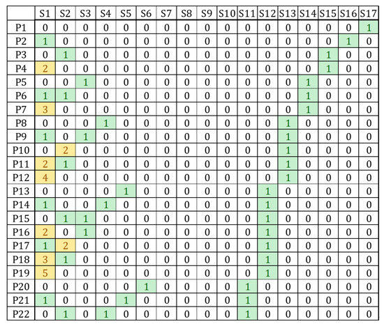
Figure 1.
Colored original pattern distribution. (First 22 patterns; green cells indicate one item in the section; yellow cells indicate more than one item in the section).
The patterns with two items are prioritized in pattern selection, since these patterns do not contain common items (Figure 2). Any change in the number of one pattern does not have an influence on other patterns. A simple vertical symmetry could be found in the chart, where the axis of symmetry lies between and .
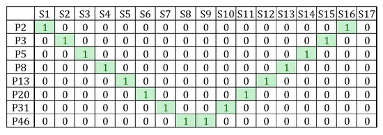
Figure 2.
Prioritized patterns (green cells).
Alternatively, we have defined sub-prioritized patterns that contain three items in each pattern (Figure 3). As marked by bold borders, a similar pattern of vertical symmetry appears in each rectangle.
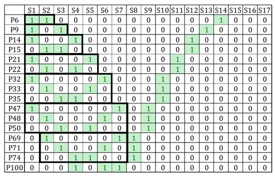
Figure 3.
Sub-prioritized patterns (The green cells in black bold boxes).
It could be hypothesized that symmetry appears regularly in the pattern discretion. As the number of sections increases, there are symmetrical patterns in different sets of pattern distribution. It is non-trivial to understand this feature: when the maximum number of items of a section of a pattern is restricted to 1, after we set the section count N, all patterns have a constraint of total size in sections of N. If we have M items including item A and item B, and sizes of other items are determined, then would be a constant under this condition. As A becomes bigger, B would become smaller.
This feature gives our algorithm an advantage in handling symmetrical distributions. For example, Figure 4. shows a normal item size distribution. If we set 10 sections for partitioning, it could be seen that the frequency in and is the same, . As and could clearly form a pattern, all patterns could be packed by patterns with a guarantee of wasted space.
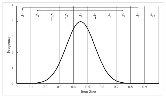
Figure 4.
Example item size distribution (normal distribution with ).
This feature would also enhance the packing of an approximately symmetrical distribution. Recall the previous example shown in Table 2. If we have accumulated some knowledge from history items and derive a prediction about the item size distribution, i.e., two items, two items, and two items, we could easily use the pattern and to guide the packing, which could generate an optimal solution.
3.3. Stability of Patterns in BPP
We deduce that patterns are stable in the solutions of BPP, so that a small error in the estimation of item distribution will only cause small deviation from optimal solutions.
Assume that the optimal solution of a BPP of n items is , where m is the number of bins used in the solution. Consider another BPP of n items in which all items are same as except one item. Let be the number of bins used in the optimal solution of . It is straightforward to deduce that is at most and at least .
Consider a solution to which uses all the patterns of . We prove that the bins used in this solution are in the worst case.
Proof: Let be the item that is different from and P be the pattern that contains in . If , , all other items can be packed into m bins according to the patterns of . So it is no more than because is at least .
If , the solution requires at most bins, while there must be . Assume that in this situation, e.g., , this is conflict with since can be packed into bins. Thus, this solution is in the worst case.
Using patterns in online BPP depends on accurate estimation of item distribution, which should be updated dynamically in the process of bin packing.
4. A Pattern-Based Algorithm for Online BPP
4.1. Algorithm
We developed a pattern-based algorithm for online BPP. This algorithm generates a plan for pattern usage based on previous distributions and packs the items according to the plan. It includes three sub-algorithms: pattern generation, pattern update and packing. In this section, this algorithm is described and evaluated.
Firstly, the data structures are explained. This algorithm keeps recording the sizes of the incoming items into the distribution according to sections S. S could be seen as equally sized intervals ranging over . is the number of intervals, which could be used to configure the algorithm. For convenience, we use to represent section n, . The range of is . An item refers to an item with size in . is a list of frequencies, with a size of . records the frequency of historical items with size in .
could be generated given and , which is the number of patterns. could be seen as a two-dimensional table, representing fixed combinations of differently sized items. The size of is . refers to the number of item in the j-th pattern. could be used to configure the algorithm.
Based on and , the pattern plan can be generated and updated. can be seen as a list of integer numbers. is the remaining quota of . Values in are decremented after patterns are applied, and updated regularly based on updated distance. The update frequency could be predefined with , which determines the number of items processed between two updates.
Bin waiting queues w are a two-dimensional array of queues, with an identical size of . is a queue of bins waiting for items. Once a new bin is generated, it is pushed into the corresponding queues. One bin may be in several queues of w. Guided by w, every bin follows an unchangeable pattern until it is fully removed from all queues. Every time an item is packed into a bin, the corresponding occurrence pops out of the queue.
As sometimes an item cannot be matched to a pattern, Best-Fit would be used as a fallback option. is a vector of all bins packed or to be packed by Best-Fit. It also receives bin packed to patterns regularly.
Secondly, the internal flow of this algorithm is explained. For clarity, we divide the entire algorithm into four parts: Main (Algorithm 1), Pattern Generation (See Appendix A: Algorithm A1), Pattern Update (See Appendix A: Algorithm A2) and Packing (See Appendix A: Algorithm A3). As can be seen in the Main function, this algorithm runs in iterations. One item is packed in one iteration. During the initialization stage, the patterns are generated, with other variables being empty or zero. In the first iteration, items are recorded into and processed by standard Best-Fit algorithm since is not yet generated and initially remains blank. Once the item counter reaches , it is reset, and the is updated based on . Then, the algorithm starts packing with patterns. The continues to accumulate, on which the is updated every items.
| Algorithm 1 Pattern-Based Online Bin Packing. |
|
The Pattern Generation function generates available patterns. It searches for possible size combinations with the priority of producing patterns with large item sizes. It starts with a pattern with single largest item type and iteratively changes the type of the smallest item one at a time. If total size of the current pattern is equal to the bin capacity, it records the pattern. If total size of the current pattern is less than the bin capacity, it duplicates the current smallest item type. If the total size of the current pattern is larger than the bin capacity, it downsizes the currently smallest item type. If the smallest item type has reached zero, the item is removed from the pattern and the second smallest item type is downsized. It stops when the current pattern is empty or the recorded pattern count has reached .
The Update Pattern plan function is to update the pattern plan based on . It scales down the historical item size distribution () to a smaller distribution () with size of , and treat this as a prediction for the next items. Based on the prediction, it generates quotas for each pattern so that most items in are prescheduled into a pattern. Note that the generation of quotas are sequential. Former patterns would be processed first. When a pattern is scheduled, the included items would be subtracted from .
The Pack Item function is to pack items into bins. After the item is classified into a section, it would firstly attempt to use patterns with large item sizes, i.e. low indices. When attempting to use a pattern, if there is a bin in the corresponding queue in w, the bin pops. If it cannot find a bin in the queue and there is still quota available in for this pattern, a new bin is created for packing and pushed into corresponding queues. If neither of two options above are available and this pattern does not include the section of this item, it attempts to use the next pattern. If no pattern is available, it falls back to use Best-Fit for packing with . When the bin is found fully packed by a pattern, it is added to .
4.2. Experiments
We have assessed the capability of this algorithm by coding with C++. First, we compare its performance with Best-Fit on Bin Usage for packing. We generate 10,000 medium-sized items with four distribution: a uniform distribution over , a triangular distribution with of 4500 over , a uniform distribution over and a triangular distribution with of 4000 over . The algorithm is configured with , , and . The result (Figure 5) shows that, on some distributions where items have medium sizes, our algorithm has an advantage in bin usage compared to Best-Fit. Note that on other distributions or with other configurations, Best-Fit might have lower bin usage.
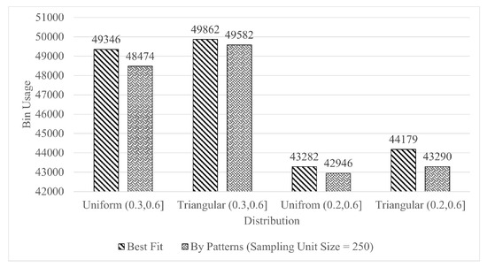
Figure 5.
Performance comparison with Best-Fit by bin usage with sampling unit size 250 on uniform and triangular distribution over and .
We compared the cause of the difference. Figure 6 shows the distribution of the wasted space of two algorithms over the uniform distribution over . It could be seen that in most of wasted space intervals, the frequency produced by our algorithm is less than Best-Fit. The overall trend is roughly a decrease in frequency as wasted space grows. The difference is that the frequency produced by Best-Fit shows a mild downward trend of frequency as waste space increases, while our algorithm gives a increase at first, followed by a sharp decrease. It means that although Best-Fit produces more accurate packing (with wasted space less than 0.05), our algorithm produces much more sub-accurate packing (with wasted space between 0.05 and 0.1). In this case, our algorithm sacrifices some possibility of packing tightest bins and largely enhances the possibility of packing bins with slightly lower tightness.
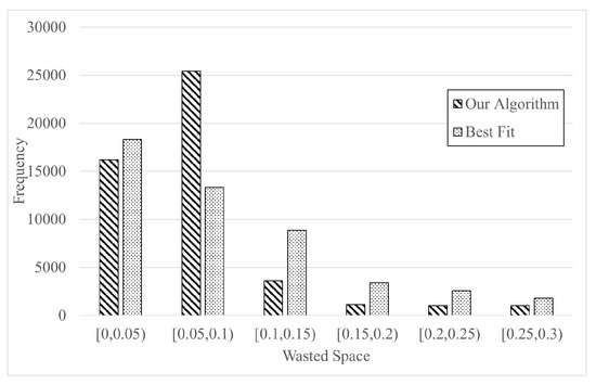
Figure 6.
Performance comparison with Best-Fit by bin wasted space with sampling unit size 250 on uniform distribution over . Intervals with frequency less than 20 are ignored.
To further investigate the behavior of our algorithm, we compared the frequency and wasted space of each type of bin in the result (Figure 7). Recall that, in the algorithm, every bin is given a category at the beginning of its packing. In this case, there are four categories of bin: bins packed by pattern 20, bins packed by pattern 31, bins packed by pattern 46 and bins packed by Best-Fit as a fallback option. It could be seen that over of bins are packed by patterns. The most used patterns are pattern 31 and pattern 46, which produce the least average wasted space. Although Best-Fit are used as a fallback option, and produces bins with higher wasted space, it does not cover the advantage brought by patterns in performance.
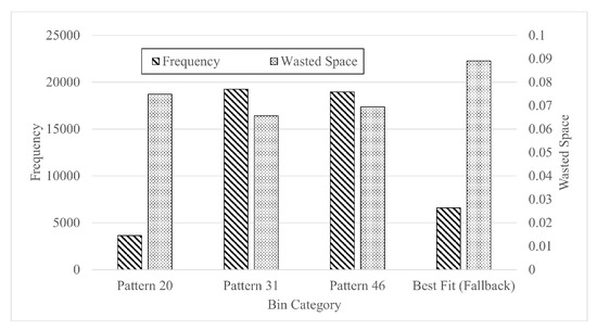
Figure 7.
Comparison between each type of bin within our algorithm with frequency and wasted space with sampling unit size 250 on uniform distribution over .
We also compare its performance with Best-Fit on CPU running time. Under the experiment settings above, on the same environment (Table 6), we repeated tests 100 times and recorded the average CPU time values. The result is shown in Figure 8. Under such circumstances, the CPU time consumed by our algorithm is to lower than that of Best-Fit.

Table 6.
Experiment environment.
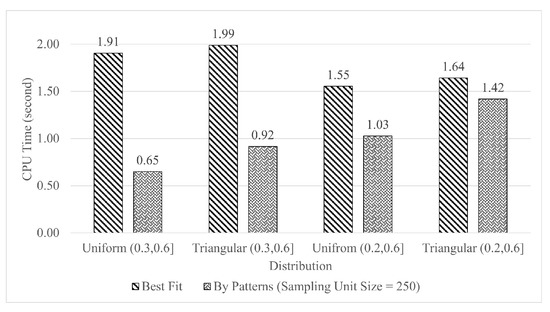
Figure 8.
Performance comparison by CPU time with sampling unit size 250 on uniform and triangular distribution over and .
In reality, the distribution of incoming item sizes is predictable based on historical data, but often changes over time. As our algorithm is based on distribution learning, distribution deviations would not change the result severely, especially when the changes are minor. An experiment designed to simulate this scenario, and to prove the feature of stability, is explained in Section 3.3. On different uniform distribution, some items are randomly selected and reassigned sizes in , which simulates changes in the distribution. With gradually deviated distributions, we record bin usage and internal pattern usage on different types of original distributions.
As can be seen in Figure 9, with the number of items with re-assigned sizes increasing, on different original distributions, the bin usage changes linearly towards the same static value, which is confirmed to be the bin usage over a uniform size distribution (0, 10,000]. This shows that a change to the original distribution would not severely degrade the performance of our algorithm. Instead, our algorithm would adapt to the change and deliver a reasonable result.
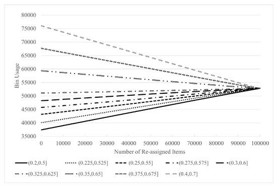
Figure 9.
Bin usage with varied uniform distributions , , , , , , , , and with sampling unit size 250; varied size over for a random Item.
A minor change to the distribution causes an even more minor change to the internal pattern usage. Figure 10 shows that, with distribution slightly changed, the internal patterns would be changed as well. However, the change is minor. Figure 11 shows that on distribution , the deviation of the overall pattern usage does not exceed the varieties of items. With deviation of item size increasing from 0 to 20, the pattern usage fluctuates between and 1. It proves that even with a varied item size, the usage of pattern is mild and stable.
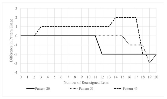
Figure 10.
Usage of pattern 19, 30 and 45 with varied uniform distributions with sampling unit size 250.
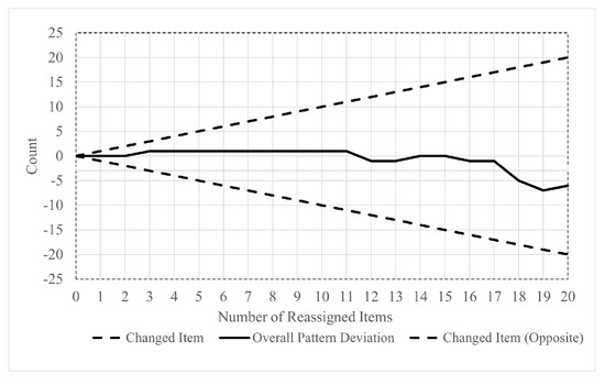
Figure 11.
Overall pattern usage with varied uniform distributions with sampling unit size 250.
5. Conclusions
In this research, we have analyzed the symmetry and stability of patterns in BPP and developed a pattern-based algorithm with parameterized symmetrical partitioning method for online BPP. The experimental results show that the proposed algorithm has a better performance for average bin usage, average wasted space and computational time compared with the heuristics of Best-Fit and First-Fit. The experiments also reveal that patterns still maintain stable in online BBP, even when the distribution varies slightly in an online BPP. This pattern based method provides a way to handle uncertainty in online BPP, which has the potential to be extended to general optimization problems with uncertainty.
The pattern-based algorithm depends on both estimation of item distribution and pattern selection. The proposed algorithm adopts heuristics to select patterns which do not compute the optimal patterns for a given distribution of items, despite the computational simplicity. This limitation may be overcome by using some meta-heuristics or machine learning methods to search pattern combinations for a given item distribution. A machine learning method may be efficient for pattern selection by computing near optimal pattern combinations with moderate computational complexity. This will be our future research focus.
Author Contributions
Software and investigation, B.L.; methodology and formal analysis, J.L.; supervision, project administration, R.B.; resources, R.Q.; validation, T.C. and H.J.; writing—original draft preparation, B.L.; writing—review and editing, J.L.; visualization, B.L.; funding acquisition, J.L. All authors have read and agreed to the published version of the manuscript.
Funding
This study is funded by a NSFC (code 72071116) and Ningbo 2025 key technology projects (code 2019B10026, E01220200006).
Institutional Review Board Statement
Not applicable.
Informed Consent Statement
Not applicable.
Data Availability Statement
Not applicable.
Conflicts of Interest
The authors declare no conflict of interest.
Appendix A
| Algorithm A1 Online Bin Packing Pattern Generation. | |
| functionGeneratePatterns (, ) | |
| initialize with size of | |
| initialize t with size of | |
| while do | |
| for all n in t do | |
| if then | ▹ Record pattern |
| for all n in t do | |
| else if then | ▹ Pattern too small |
| if then | ▹ Duplicate |
| else | ▹ Remove item |
| else | ▹ Pattern too large |
| ▹ Downsize | |
| return | |
| Algorithm A2 Online Bin Packing Pattern Update. | ||
| functionUpdatePatternPlan (,) | ||
| initialize | ||
| for to do | ▹ Generate prediction | |
| initialize | ||
| for to do | ▹ Generate pattern plan | |
| for to do | ||
| if then | ||
| if then | ||
| if then | ||
| for to do | ||
| return | ||
| Algorithm A3 Online Bin Packing Pack by Patterns. | |
| functionPackItem (,,,, w, ) | |
| initialize current bin b as | |
| for to do | |
| if then | |
| if then | |
| else if then | |
| for to do | |
| for to do | |
| if then | |
| if then | |
| if then | |
References
- Johnson, D.S.; Demers, A.; Ullman, J.D.; Garey, M.R.; Graham, R.L. Worst-Case Performance Bounds for Simple One-Dimensional Packing Algorithms. SIAM J. Comput. 1974, 3, 299–325. [Google Scholar] [CrossRef] [Green Version]
- Johnson, D.S. Fast algorithms for bin packing. J. Comput. Syst. Sci. 1974, 8, 272–314. [Google Scholar] [CrossRef] [Green Version]
- Johnson, D.S. Near-Optimal Bin Packing Algorithms. Ph.D. Thesis, Massachusetts Institute of Technology, Cambridge, MA, USA, 1973. [Google Scholar]
- Yao, A.C.-C. New Algorithms for Bin Packing. J. ACM 1980, 27, 207–227. [Google Scholar] [CrossRef] [Green Version]
- Coffman, E.G.; Csirik, J.; Galambos, G.; Martello, S.; Vigo, D. Bin Packing Approximation Algorithms: Survey and Classification. In Handbook of Combinatorial Optimization; Springer: New York, NY, USA, 2013; pp. 455–531. [Google Scholar]
- Lee, C.C.; Lee, D.T. A simple on-line bin-packing algorithm. J. ACM 1985, 32, 562–572. [Google Scholar] [CrossRef]
- Ramanan, P.; Brown, D.J.; Lee, C.C.; Lee, D.T. On-line bin packing in linear time. J. Algorithms 1989, 10, 305–326. [Google Scholar] [CrossRef] [Green Version]
- Richey, M.B. Improved bounds for harmonic-based bin packing algorithms. Discret. Appl. Math. 1991, 34, 203–227. [Google Scholar] [CrossRef] [Green Version]
- Seiden, S.S. On the online bin packing problem. J. ACM 2002, 49, 640–671. [Google Scholar] [CrossRef]
- Balogh, J.; Békési, J.; Galambos, G. New lower bounds for certain classes of bin packing algorithms. Theor. Comput. Sci. 2012, 440–441, 1–13. [Google Scholar] [CrossRef] [Green Version]
- Heydrich, S.; van Stee, R. Beating the Harmonic Lower Bound for Online Bin Packing. In Proceedings of the 43rd International Colloquium on Automata, Languages, and Programming (ICALP 2016), Rome, Italy, 12–15 July 2016; pp. 41:1–41:14. Available online: http://drops.dagstuhl.de/opus/volltexte/2016/6321 (accessed on 10 December 2021).
- Silva-Gálvez, A.; Lara-Cárdenas, E.; Amaya, I.; Cruz-Duarte, J.M.; Ortiz-Bayliss, J.C. A Preliminary Study on Score-Based Hyper-heuristics for Solving the Bin Packing Problem. In Pattern Recognition; Lecture Notes in Computer Science; Springer Science+Business Media: Berlin/Heidelberg, Germany, 2020; Chapter 30; pp. 318–327. [Google Scholar]
- Dunke, F.; Nickel, S. A data-driven methodology for the automated configuration of online algorithms. Decis. Support Syst. 2020, 137, 113343. [Google Scholar] [CrossRef]
- Gupta, V.; Radovanović, A. Interior-Point-Based Online Stochastic Bin Packing. Oper. Res. 2020, 68, 1474–1492. [Google Scholar] [CrossRef]
- Ross, N.; Keedwell, E.; Savic, D. Human-Derived Heuristic Enhancement of an Evolutionary Algorithm for the 2D Bin-Packing Problem. In Parallel Problem Solving from Nature—PPSN XVI; Springer: Cham, Switzerland, 2020; pp. 413–427. [Google Scholar]
- Zhao, H.; She, Q.; Zhu, C.; Yang, Y.; Xu, K. Online 3D bin packing with constrained deep reinforcement learning. In Proceedings of the AAAI Conference on Artificial Intelligence, Virtually, 2–9 February 2021; AAAI Press: Palo Alto, CA, USA, 2021; Volume 35, pp. 741–749. [Google Scholar]
Publisher’s Note: MDPI stays neutral with regard to jurisdictional claims in published maps and institutional affiliations. |
© 2022 by the authors. Licensee MDPI, Basel, Switzerland. This article is an open access article distributed under the terms and conditions of the Creative Commons Attribution (CC BY) license (https://creativecommons.org/licenses/by/4.0/).